
Submitted:
07 July 2025
Posted:
08 July 2025
You are already at the latest version
Abstract
The effect of temperature change on the change of modal frequencies leads to erroneous results in the detection of structural damages. Therefore, measuring the temperature effect on modal frequencies is a critical step to eliminate errors in damage detection. Due to the irregular and time-dependent temperature distribution properties, it is not possible to obtain reliable relationships between temperatures and modal frequencies by using air or surface temperatures. In order to determine this relationship, changes in the dynamic parameters of the steel benchmark structure were observed by performing operational modal analysis of +2 and +32 degrees. Shaking table was used to obtain the parameters. Micro tremor data recorded from the ground level were used in the measurements as ambient vibration. For the evaluation of measurement data, EFDD, which is used as FDD, EFDD and SSI methods, has been chosen and dynamic parameters have been obtained. Similar results were obtained for different temperature values. While there was an exact match between mode shapes, there was an average difference of 2.43% between frequencies. It has been determined that the dynamic parameters obtained as a result of the operational modal analysis have a linear relationship with the temperature change.
Keywords:
experimental modal analysis
; modal parameter
; EFDD
; temperature
1. Introduction
In Civil Engineering structures, increasing the dimensions of the building and the loads to the elements will increase the dimensions of the elements in the system and thus an economic and suitable design is not possible. Therefore, structures are considered ductile under earthquake loads and structures are designed for reduced elastic earthquake loads. Damage to existing structures is inevitable since the earthquake is considered to be at the beginning of the design which will be damaged by showing the linear behavior. Damage to existing buildings is not caused by earthquakes. Excavations around the building, tunnel and subway constructions and blasting activities can also occur when conditions are encountered that adversely affect the stability of the building (Lenza et al. 2017). Therefore, the damage assessment in existing buildings should be monitored throughout the life of the building. The purpose of the study, load distribution or structural system will be changed, pre-earthquake or after the performance of the existing buildings to be evaluated and strengthened to perform and very detailed studies are obtained from these studies. For this reason, there is a need for a method to accelerate the damage detection studies applied to the risky buildings (De Canio et al. 2016). Operational Modal Analysis is the most preferred method that provides dynamic parameters to be measured by measuring the effects of ambient vibrations on structures.
The operational modal analysis method is the preferred method for determining the current performance levels of many types of structure due to its ease of application and its interactive solution with the ground. In order to determine the material performance, it is not necessary to take material samples from the building and to take ground samples in order to determine the building performance level (Nezhad and Poursha, 2015). The operational modal analysis method simplifies these detailed studies to provide faster and more accurate results. In order to determine the behavior of the structures under the effect of dynamic loads, it is necessary to determine the mode shapes, natural frequencies and damping ratios which are the dynamic parameters of the structures (Zhu et al. 2015; Basaran et al. 2015). In buildings, there are structural differences due to differences between project and application, damage or reinforcement. The dynamic characteristics of the building vary with these changes. By following the differences in the dynamic characteristics, it is possible to get an idea about the stiffness of a building and the change in the level of damage (Ni et al. 2015).
In general, operational modal analysis is used to determine the damage levels of the existing structures, to check the validity of the assumptions made while constructing the finite element model, to update the initial numerical model of the existing structures according to the experimental data, to determine the dynamic characteristics of the structures by the experimental modal analysis method when the numerical model of the existing structures cannot be formed and to follow the structural health is widely used in the process (Tseng et al. 1994; Aliev and Larin 1998; Ljung, 1999; Roeck, 2003). It was observed that three types of definitions were used in the engineering structures: modal parameter identification; structural-modal parameter identification; control-model identification methods are used. In the frequency domain the identification is based on the singular value decomposition of the spectral density matrix and it is denoted Frequency Domain Decomposition (FDD) and its further development Enhanced Frequency Domain Decomposition (EFDD). In the time domain there are three different implementations of the Stochastic Subspace Identification (SSI) technique: Unweighted Principal Component (UPC); Principal component (PC); Canonical Variety Analysis (CVA) is used for the modal updating of the structure (Friswell and Mottershead, 1995; Marwala, 2010). It is necessary to estimate sensitivity of reaction of examined system to change of random or fuzzy parameters of a structure. Investigated measurement noise perturbation influences to the identified system modal and physical parameters. Estimated measurement noise border, for which identified system parameters are acceptable for validation of finite element model of examine system. System identification is realized by observer Kalman filter (Kalman, 1960; Ibrahim, 1977; Juang et al.; 1993) and Subspace algorithms (Overschee and De Moor, 1996). In special case observer gain may be coincide with the Kalman gain. Stochastic state-space model of the structure are simulated by Monte- Carlo method. As a result of these theoretical and experimental studies, the importance of temperature change and humidity has emerged once again from the environmental factors affecting the modal parameters. The effects of temperature and humidity on modal parameters have been the subject of thorough examination in the last 15 years (Kasimzade and Tuhta, 2007a; 2007b; 2009). Many structures of steel, reinforced concrete and composite materials related to the effect of temperature and humidity change on modal parameters have been investigated. These examinations were conducted daily, weekly and monthly. Changes in temperature and humidity were evaluated in three different ways. The first is the ambient temperature and humidity, the other is the temperature and humidity of the building and the last is the surface temperature and humidity of the building. Analyzes were repeated for different situations. As a result of these analyzes, the relationship between the changes in the modal parameters for different temperature and humidity values was tried to be determined. It was clearly shown that modal frequencies decreased with the increasing of temperature (Kakar and Kakar, 2015).
The Quanser Shake Table is a bench-scale earthquake simulator ideal for teaching structural dynamics, control topics related to earthquake, aerospace and mechanical engineering and widely used in applications. In this study was investigated of possibility using the recorded micro tremor data on ground level as ambient vibration input excitation data for investigation and application Experimental Modal Analysis (EMA) on the bench-scale earthquake simulator (The Quanser Shake Table) for steel benchmark structures.
For this purpose, operational modal analysis of a steel benchmark structure for dynamic parameters was evaluated at two temperatures (+2 and +32 degrees). Ambient excitation was provided by shake table from the recorded micro tremor ambient vibration data on ground level. Enhanced Frequency Domain Decomposition is used for the output only modal identification.
2. Possible Effects of Temperature on SHM Systems through Dynamic Parameters
This section summarizes Structural Health Monitoring (SHM) systems. In this study, only the effect of temperature on dynamic parameters was examined in terms of application. SHM systems must have the ability to distinguish environmental effects. Otherwise, especially factors such as frequency changes due to temperature may interfere with measurements for damage detection. Therefore, the effect of temperature on frequency and damping ratios was tested experimentally in this study. Thus, it is aimed to contribute to the modal analysis methods used within the scope of SHM. SHM Systems include continuous observation of structural performances against damage effects occurring in structures over time and evaluation of structural health with the obtained measurements. However, it also records environmental effects. These systems are of vital importance in large and important critical structures. In these systems, vibration and dynamic behaviors are detected by accelerometers, deformations are measured by strain gauges (Sevieri and De Falco, 2020), and displacements are measured by LVDTs (Noel et al., 2017). Temperature effects from environmental factors are measured by thermocouple/heat sensors (Avci et al., 2021). Fiber optic sensors are used for high-accuracy long-distance measurements (Park et al., 2013). All these measured data are collected, filtered, and stored by wireless sensor networks (WSN) or wired systems. Data processing and analysis software are used to perform modal analysis of the structural system, determine frequency changes, and calculate the damage index. Among all these processes, determining temperature changes is especially important for the healthy interpretation of other measurements. At this point, compensation techniques have been developed to eliminate temperature effects with artificial intelligence and machine learning trained with statistical analysis. Thus, it can be determined with high accuracy whether the structure is really damaged or not. Errors that may occur in decisions such as maintenance, reinforcement or evacuation decisions are eliminated. The purpose of SHM systems is to detect structural damage early, reduce maintenance costs, perform real-time risk assessment, verify performance-oriented design and ensure safety assessment after dynamic effects. Therefore, possible deviations from this goal are reduced.
In SHM systems, dynamic-based methods based on vibration data such as modal frequency, shape and damping ratio analyses are used. Thus, if there is damage in the structure, it is determined that the frequency decreases and the mode shapes change. In SHM systems, static loading-based methods such as monitoring strain and displacement data are also evaluated. The finite element model is compared with the real structure. Statistical inferences are made from long-term measurement data. However, while performing all these operations, environmental effects such as temperature must be separated. Sohn et al. (2004), who proposed statistical methods to separate the effect of temperature on frequencies, classified SHM methods and discussed the effects of environmental factors such as temperature and humidity on signal variation in long-term field applications. Farrar and Worden (2007), who presented the basic concepts, development and classifications of SHM, especially focused on the effects of environmental changes on modal parameters and emphasized how these effects can be misleading in damage detection. Lin et al. (2011) used SHM systems for seismic monitoring and wind loads in the Taipei 101 building in Taiwan. The effects of wind gusts and the Wenchuan earthquake on the structure were monitored using 30 accelerometers in Taipei101. The obtained natural frequency and mode shapes showed the effects of temperature and environmental changes on the dynamic behavior. The system was able to monitor the performance of the structure under real-time seismic and wind loads via SHM. Tcherniak and Mølgaard (2015) performed a vibration stimulation with an actuator placed inside the blade in an experiment carried out on a 34 m long wind turbine blade. Despite the effect of ambient temperature, they were able to successfully detect pre-damage cracks with artificial neural networks through the measured vibrations. A system that can distinguish crack-free structures was established by including the temperature-vibration relationship in the SHM model. Thus, rotor blade vibrations and temperature effects were examined together and pre-crack detections were made accurately. Li et al. (2023) monitored the temperature and vibration behavior of the structure in real time using distributed fiber optic temperature and strain sensors on the Sutong Bridge in China. They showed that the measured mode frequencies without isolation showed a significant relationship with temperature and that temperature effects can cause significant deviations in SHM analyses. As a result, it can be said that although SHM systems are indispensable tools of modern engineering, environmental effects such as temperature compensation must be eliminated by methods such as statistical modeling and machine learning.
Especially in steel structures, temperature affects the structural stiffness by changing the Young modulus. This change can cause serious deviations in modal frequencies. For example, Serker and Wu (2009) investigated the changes in modal frequencies due to temperature by conducting experiments on a simply supported steel beam. The results showed that the frequency changes caused by moderate structural damage can be at the same or greater levels than the temperature changes. In other words, the frequency deviations due to temperature are large enough to cause confusion during damage detection. This is an indication that the reliability of modal-frequency based SHM methods applied without considering the temperature effect may be low. Xia et al. (2012) investigated the effects of temperature on vibration properties such as modal frequency, shape and damping in literature review and case studies. The analyses showed that temperature changes significantly changed the dynamic parameters in steel structures and thin members such as reinforced concrete slabs. It was determined that the changes in structural vibration properties due to temperature changes can be more significant than the changes caused by moderate structural damage. Luo et al. (2022) also emphasizes that modal variables should not be confused with temperature and states that based on literary data, temperature effects can be equivalent to structural damage. All of this shows that temperature effects should not be ignored in SHM analyses. In this case, devices used for SHM applications should model or normalize the temperature-data relationship instead of only monitoring frequency changes. Otherwise, temperature changes may lead to false damage detections.
In large-scale structures, the temperature distribution is irregular on the surface. It is a time-dependent process that includes internal-external differences. Therefore, reliability cannot be achieved with measurements in determining the temperature-frequency relationship. Because the surface/core temperature may be different in different regions of the steel structure; temperature transition occurs with a delay in time (Thermal gradients). In addition, if the supports in steel systems are displaced due to the effect of temperature, the modal behavior also changes (Change of boundary conditions). For these reasons, it is not possible to represent the real thermal situation on the entire structure by measuring only the air and surface temperatures. To overcome these problems, Bao et al. (2017) used fiber optic sensors as distributed temperature sensors to fully monitor both internal and external temperatures. Wang et al. (2020) monitored a laboratory-scale RC plate for 1 year and collected data on natural frequency, mode shapes and damping ratios depending on the average temperature values changing over time. Statistical/graded models (LR, ARX, ARIMA) such as the ARX+PSO approach were used to neutralize the temperature effect and detect damage. These models were trained with data obtained from the undamaged structure and defined with confidence intervals. The results showed that the expected damage levels were correctly determined with this method. This study is an example that shows that the temperature effect can be systematically and reliably separated in the SHM literature; moreover, the ARX+PSO combination can correctly define the changes on the mode frequencies as “damage” or “environmental change”. As a result, it was determined in the study that temperature changes create significant fluctuations in natural frequencies and their effect on the mode shape and damping is limited. In the study of Venglar & Lamperova (2021), it was observed that some natural frequencies increase with increasing temperature, while other modes decrease. For example, while the frequency of the first two modes increases, the frequency of the fourth mode decreases. This situation shows that there may be nonlinear behaviors in the temperature-frequency relationship. Wang et al. (2021) experimentally applied gradual temperature gradients ranging from 10–30°C on the bridge deck element, and the sample was tested under different support conditions. The same temperature loading conditions were modeled with the ABAQUS FE model through heat transfer simulation. The temperature field obtained as a result of FE was analyzed based on stress and possible modal properties and compared with experimental observations. Determination of the real temperature field with FE provides accuracy since it is based on the thermal distribution representing the entire thickness of the structure instead of just the air temperature. The application of heat transfer, thermal expansion and modal analysis stages together realistically captures the effect of temperature changes on modal frequencies. The fact that the obtained results are generally compatible with experimental data with deviations below 1% supports the usability of such models in practical SHM applications. Kamei et al. (2021) experimentally investigated the effect of the temperature increase rate on the modal behavior of a steel cantilever beam. In the study, the characterization of the dynamic changes in the period until isothermal (constant temperature) conditions were obtained was determined. Controlled temperature was applied to the structure at different heating rates (low, medium and high). Under each heating rate, the system was tested with modal analysis when the structure reached a certain temperature. After the relevant temperature was kept constant, vibration data were collected and natural frequencies were calculated. The heat increase was achieved with controlled heaters rather than external environment. As a result, a significant decrease was observed in natural frequencies due to temperature increase. However, even if the same final temperature was reached, different heating rates affected the modal responses of the system differently. In other words, the temperature change rate stood out as a parameter as important as the temperature itself. It was concluded that at high heating rates, transient thermal stresses and temperature gradients were greater, and therefore larger deviations occurred in frequencies. This study shows that in SHM applications, not only the instantaneous value of the temperature but also the transition process should be taken into account. Therefore, these results show that models such as ARX and ARIMA, which try to neutralize temperature effects, should also include heating curves and thermal lag effects.
Poudel et al (2024) modeled the temperature-frequency dependency by entering the real temperature distribution into the structural model with FE analyses performed together with experimental tests. First, the temperature distribution from 20 to 50°C on the real steel-concrete composite beam sample was calculated with heat transfer and thermal expansion analyses in the FE model. Then, the obtained temperature field was used in the modal analysis and the natural frequencies were evaluated. FE results coincided with the experimental frequency values with high accuracy (±0.06% deviation). Poudel et al (2024) based their study on a simply supported cantilevered steel beam. In the experiments, a decrease of approximately 0.44% was observed in the second bending mode frequency as the temperature increased by 1°C. This experimental study shows that both the frequency decreases as the temperature increases and the modal amplitude decreases. It is also understood from the study that the temperature increase rate may also be effective. In the light of all this information, it can be said that if the temperature effects are neglected, serious errors are inevitable in SHM systems. Distributed temperature measurement and modeling are required to establish the temperature-frequency relationship reliably. Experimental data show that the general trend is a decrease in frequency as the temperature increases, but an increase in the frequency of some modes can also be observed in some structure/geometry combinations.
3. Materials and Methods
3.1. Modal Parameter Extractions
The EFDD technique used in SHM system applications was preferred in this study and used as the basic data generator to understand the effect of temperature changes on frequency and damping ratios. Thus, the sensitivity of modal parameters, which are the basic data source of statistical or artificial intelligence-based compensation methods for eliminating temperature-related errors in SHM applications, was evaluated. Similar to studies such as Poudel et al. (2024) and Wang et al. (2020) that directly model the temperature-frequency relationship in SHM, this study also aimed to analyze the temperature effect directly through frequency shifts
The (FDD) ambient modal identification is an extension of the Basic Frequency Domain (BFD) technique or called the Peak-Picking technique. This method uses the fact that modes can be estimated from the spectral densities calculated, in the case of a white noise input, and a lightly damped structure. It is a non parametric technique that determines the modal parameters directly from signal processing (Lus et al. 2003). The FDD technique estimates the modes using a Singular Value Decomposition (SVD) of each of the measurement data sets. This decomposition corresponds to a Single Degree of Freedom (SDOF) identification of the measured system for each singular value (Lam and Yang, 2015; Brincker et al. 2000). The Enhanced Frequency Domain Decomposition technique is an extension to Frequency Domain Decomposition (FDD) technique. This t technique is a simple technique that is extremely basic to use. In this technique, modes are easily picked locating the peaks in Singular Value Decomposition (SVD) plots calculated from the spectral density spectra of the responses. FDD technique is based on using a single frequency line from the Fast Fourier Transform analysis (FFT), the accuracy of the estimated natural frequency based on the FFT resolution and no modal damping is calculated. On the other hand, EFDD technique gives an advanced estimation of both the natural frequencies, the mode shapes and includes the damping ratios (Jacobsen et al. 2006). In EFDD technique, the single degree of freedom (SDOF) Power Spectral Density (PSD) function, identified about a peak of resonance, is taken back to the time domain using the Inverse Discrete Fourier Transform (IDFT). The natural frequency is acquired by defining the number of zero crossing as a function of time, and the damping by the logarithmic decrement of the correspondent single degree of freedom (SDOF) normalized auto correlation function (Peeters, 2000; Bendat,1998).
In this study modal parameter identification was implemented by the Enhanced Frequency Domain Decomposition. The relationship between the input and responses in the EFDD technique can be written as, In this method, unknown input is represented with “x” (“t” ) and measured output is represented with “y” (“t” )
Where “G” _”xx” “(jω)” is the r x r Power Spectral Density (PSD) matrix of the input. “G” _”yy” “(jω)” is the m x m Power Spectral Density (PSD) matrix of the output, “H(jω)” is the m x r Frequency Response Function (FRF) matrix, and * superscript T denote complex conjugate and transpose, respectively. The FRF can be reduced to a pole/residue form as follows:
Where n is the number of modes “λ” _”k” is the pole and, R_k is the residue. Then Eq. (1) becomes as:
Where s the singular values, superscript is H denotes complex conjugate and transpose. Multiplying the two partial fraction factors and making use of the Heaviside partial fraction theorem, after some mathematical manipulations, the output PSD can be reduced to a pole/residue form as fallows;
Where “A” _”k” is the k th residue matrix of the output PSD. In the EFDD identification, the first step is to estimate the PSD matrix. The estimation of the output PSD known at discrete frequencies is then decomposed by taking the SVD (singular value decomposition) of the matrix;
Where the matrix is a unitary matrix holding the singular vectors and is a diagonal matrix holding the scalar singular values. The first singular vector is an estimation of the mode shape. PSD function is identified around the peak by comparing the mode shape estimation with the singular vectors for the frequency lines around the peak. From the piece of the SDOF density function obtained around the peak of the PSD, the natural frequency and the damping can be obtained.
3.2. Description of Steel Benchmark Structure
The Quanser shake table II is a uniaxial bench-scale shake table. This unit can be controlled by appropriate software was illustrated in Figure 1a,b. It is effective for a wide variety of experiments for civil engineering structures and models. Shake table specifications are as follows Table 1 (Quanser, 2008).
Steel benchmark structure is 1.00 m height. Thickness of elements is 0.0015 m. The structure dimensions are shown in Figure 2.
The steel system used is made of galvanized steel and its chemical composition is given in Table 2. Galvanized steel is a material obtained by protecting the steel surface with zinc coating. It provides advantages in long-term experimental studies or in outdoor conditions due to its resistance to corrosion. By choosing galvanized steel as the material in this study, it became possible to observe the effect of temperature effects directly on steel elasticity (Young’s Modulus). If a different quality steel that is prone to rust and age was used, this effect could be noisy. In addition, the surface reflectivity of galvanized steel reduces thermal transmittance; this can soften the effects of thermal gradient. Thus, problems such as temperature difference between the inner-core and outer surface occurred less in the tested system. Since the chemical composition of galvanized steel (Table 2) is low-carbon and low-alloyed, its mechanical properties are more sensitive to temperature. This makes it easier to capture dynamic frequency changes. Poudel et al. (2024) and Serker & Wu (2009) also stated that the temperature-frequency relationship can be observed more clearly with low-carbon steel or zinc-coated samples. Thanks to the galvanized coating, the outer surface of the structure is less affected by temperatures. This allows the internal structure to show a more stable frequency characteristic. In this way, galvanized steel offers the opportunity to clearly observe the expansion and elasticity changes caused by temperature. The thermal behavior of the material is of critical importance in order to distinguish the effects of temperature changes in SHM systems. Galvanized steel elements allow reliable vibration data to be collected without material deterioration (e.g. rust, surface roughness) in long-term SHM applications. The suppression of the moisture effect due to the coating also facilitates the separation of the mixed effects of temperature and moisture in SHM systems. In the study of Xia et al. (2012), the response of steel structures to temperature differed according to the material type. More stable mode shapes were observed in galvanized samples. Luo et al. (2022) points out that controlled surface systems such as galvanized are easier to model in SHM algorithms.
The coordinates of the point where the experiments were conducted in Samsun province of Turkey are 41.3623618; 36.1836511. Figure 3. shows the monthly average temperature changes in Samsun province of Turkey (Climate-Data.org., n.d.)., where the experiment was conducted, between 1991 and 2021. Since the largest temperature difference is between January and August, the dates of the experiments were determined in this way.
4. Analysis of Experimental Results
4.1. Experimental Modal Analysis of Steel Benchmark Structure at +2 °C Degrees
Experimental modal analysis of steel benchmark structure at different temperatures was performed. The temperature values have been determined by considering the long annual data. According to these data, the first measurement was made on 13.01.2024 when the ambient temperature was +2 degrees. Ambient excitation was provided by the recorded micro tremor data on ground level. Three accelerometers (with both x and y directional measures) were used for the ambient vibration measurements, one of which were allocated as reference sensor always located in the first floor (they are shown by the red line in Figure 4a, b). Two accelerometers were used as roving sensors (they are shown by the black line in Figure 4a, b). The response was measured in two data sets (Figure 4a, b). For two data sets were used 3 and 5 degree of freedom records respectively (Figure 4a, b). Every data set (Figure 4a, b) was measured 100 min. The selected measurement points and directions are shown in Figure 4a, b.
The data acquisition computer was dedicated to acquiring the ambient vibration records. In between measurements, the data files from the previous setup were transferred to the data analysis computer using a software package. This arrangement allowed data to be collected on the computer while the second, and faster, computer could be used to process the data in site. This approach maintained a good quality control that allowed preliminary analyses of the collected data. If the data showed unexpected signal drifts or unwanted noise or for some unknown reasons, was corrupted, the data set was discarded and the measurements were repeated (Figure 5a, b).
Before the measurements could begin, the cable used to connect the sensors to the data acquisition, equipment had to be laid out. Following each measurement, the roving sensors were systematically located from floor to floor until the test was completed. The equipment used for the measurement includes three quanser accelerometers (with both x and y directional measures) and geosig uni-axial accelerometer, matlab data acquisition toolbox (wincon). For modal parameter estimation from the ambient vibration data, the experimental modal analysis (EMA) software ARTeMIS Extractor (1999) is used.
The simple peak-picking method (PPM) finds the eigenfrequencies as the peaks of nonparametric spectrum estimates. This frequency selection procedure becomes a subjective task in case of noisy test data, weakly excited modes and relatively close eigenfrequencies. Also for damping ratio estimation the related half-power bandwidth method is not reliable at all. Frequency domain algorithms have been the most popular, mainly due to their convenience and operating speed.
Singular values of spectral density matrices, attained from vibration data using PP (Peak Picking) technique are shown in Figure 6. Natural frequencies acquired from the all measurement setup are given in Table 3. The first five mode shapes extracted from experimental modal analyses are given in Figure 7. When all measurements are examined, it can be seen that there are best accordance is found between experimental mode shapes (+2 °Cand +32 °C degrees). When the experimentally identified modal parameters are checked with each other, it can be seen that there is a best agreement between the mode shapes in experimental modal analyses at +2 °Cand +32 °C degrees. (Table 5).
4.2. Experimental Modal Analysis of Steel Benchmark Structure at +32 °C Degrees
Experimental modal analysis of steel benchmark structure at different temperatures was performed. The temperature values have been determined by considering the long annual data. According to these data, the second measurement was made on 20.08.2024 when the ambient temperature was +32 degrees.
Measurements at +32 degrees Celsius were repeated for this temperature. Singular values of spectral density matrices, attained from vibration data using PP (Peak Picking) technique are shown in Figure 8. Natural frequencies acquired from the all measurement setup are given in Table 4. The first five mode shapes extracted from experimental modal analyses are given in Figure 9. When all measurements are examined, it can be seen that there are best accordance is found between experimental mode shapes (+2 °C and +32 °C degrees). When the experimentally identified modal parameters are checked with each other, it can be seen that there is a best agreement between the mode shapes in experimental modal analyses at +2 °Cand +32 °C degrees. (Table 5).

Table 4.
Experimental modal analysis result at the steel benchmark structure at +32 °C.
| Mode number | 1 | 2 | 3 | 4 | 5 |
| Frequency (Hz) | 2.017 | 5.725 | 6.828 | 7.770 | 8.987 |
| Modal damping ratio (ξ) | 0.672 | 1.822 | 1.035 | 0.551 | 0.670 |
Table 5.
Comparison of experimental modal analysis results.
| Mode number | 1 | 2 | 3 | 4 | 5 |
| Experimental frequency (Hz) +2°C | 2.067 | 5.868 | 6.998 | 7.964 | 9.211 |
| Experimental frequency (Hz) +32°C | 2.017 | 5.725 | 6.828 | 7.770 | 8.987 |
| Difference (%) | 2.418 | 2.436 | 2.429 | 2.435 | 2.431 |
5. Results
In this study, the effect of temperature change of steel benchmark structure on modal parameters was investigated using Quanser Shake Table.
The ambient vibration tests are conducted under provided by shake table from ambient vibration data on ground level. Modal parameter identification was implemented by the Enhanced Frequency Domain Decomposition (EFDD) technique.
For this purpose, modal parameters obtained at +2 0C and +32 0C degrees were compared on shake table with ambient vibrations.
From +2 0C degrees steel benchmark structure a total of five natural frequencies were attained experimentally, which range between 2.067 and 9.211 Hz.
From +32 0C degrees steel benchmark structure a total of five natural frequencies were attained experimentally, which range between 2.017 and 8.987 Hz.
Experimental modal frequencies differences were found separately for each mode. The frequency differences caused by the temperature 30 0C change were observed to be approximately %2.4.
In this study, in the experiments conducted at 30 °C differences, the decrease in frequencies while the mode shapes remained constant could be revealed in a transparent and predictable way thanks to the homogeneous structure of the galvanized steel. If a different and deterioration-prone steel had been used, the changes in frequency could have been more complex or uncertain due to thermal expansion irregularities, temperature conduction differences, and the effects of internal structural errors. The use of galvanized steel in the study was an important choice in terms of isolating and reliably revealing the effects of temperature changes on dynamic parameters. The elimination of corrosion effects thanks to its coated structure, the more compatible surface temperature with the core part of the structure, and the sensitive responses of its low-carbon structure to elasticity changes allowed the changes in modal frequencies to be observed clearly.
Presented investigation results are shown and confirm of possibility using the recorded micro tremor data on ground level as ambient vibration input excitation data for investigation and application Experimental Modal Analysis (EMA) on the bench-scale earthquake simulator (The Quanser Shake Table) for steel benchmark structures and shed light on the development of related research. It was clearly seen that the frequency decreases with increasing temperature.
As the temperature increased, the frequency decreased in all modes. This situation is parallel to the literature (Poudel et al., 2024; Wang et al., 2020). The decrease in the first mode (~0.05 Hz) indicates a decrease in the stiffness of the structure. This can be explained by the decrease in the Young modulus with the increase in temperature. However, the decrease in the 4th and 5th modes is more pronounced (about 0.22 Hz). This may indicate that high-frequency modes are more sensitive to temperature changes. The mode shapes were not affected by the temperature change. This shows that the frequency changes are related to the changes in material elasticity rather than the boundary conditions. The damping ratios remained constant. This shows that the temperature change does not have a serious effect on the damping. In the studies conducted by Xia et al. (2012) and Luo et al. (2022), it is seen that the temperature affects the frequency but the damping ratios do not change much. In parallel with the results obtained in this study, corresponding researches have also demonstrated that mode shapes are not sensitive to temperature variation, and the change of modal damping may be masked by measurement noise (Balmès et al., 2008; Xia et al., 2006; Moser and Moaveni, 2011). The frequency decrease of approximately 2.4% observed for all five modes reveals that temperature-induced frequency shifts should not be confused with structural damage in SHM applications. Similarly, it has been reported in the literature (Poudel et al., 2024; Serker and Wu, 2009) that temperature changes create similar effects to moderate structural damage. Therefore, performing damage detection directly by frequency monitoring without temperature compensation in SHM systems may be misleading. Based on this study and the relevant literature, it is possible to suggest some numerical values for the relationship between the percentage change of temperature and the percentage change rate in frequencies. However, the general validity and practical benefits of such suggestions will vary, especially depending on the building materials, structural geometries, environmental factors and SHM techniques used. Different types of materials respond to temperature changes in different ways. In addition, the effect of temperature change varies not only with air temperature but also with environmental factors such as humidity, wind and solar radiation. Therefore, temperature-frequency ratios should be based on specific environmental conditions. In addition, large-scale structures may cause more significant frequency changes due to temperature expansion. Therefore, frequency change rates between small and large structures may also differ. In addition, temperature changes that will occur under high temperatures may cause larger changes in frequencies. As a result, specific temperature-frequency modeling should be performed for each structure and environment. However, as an approximate suggestion, since approximately 2.4% frequency decrease was determined in each mode at a temperature difference of 30°C from this study, it can be said that a 1°C temperature increase creates a 0.15% frequency decrease. This situation suggests that temperature increase causes a decrease in modal frequencies almost linearly. Some studies report that temperature increase in single steel elements or complex structural systems causes a certain decrease in frequencies (e.g., Serker & Wu, 2009; Poudel et al., 2024), and it has been reported that in some experiments, a decrease of 0.1–0.5% in frequency can be observed for a 1°C increase.
Based on experimental data, a simple linear model can be proposed as ∆f/f≈k.∆T/T, where f: Initial frequency, ∆f: frequency change, T: initial temperature, ∆T: temperature change and k: a constant that varies according to material properties (e.g., Young’s modulus change with temperature), structural properties (element thickness, connection type) and boundary conditions. In some cases, especially in wide temperature ranges, it may be necessary to use nonlinear models. In these models, the change in the elastic properties of the material with increasing temperature can be reflected more accurately. In such cases, polynomial or exponential functions determined by experimental calibration can be used. Therefore, although the recommendations serve as a general guide, they will first require laboratory and field calibration for each structure. Models to be used in SHM systems in particular should be re-adjusted according to the unique properties of the structure (e.g., with local temperature measurements and modal parameter tracking) and model validity should be continuously checked. In summary, the numerical values that can be suggested for the percentage change rate of frequency change depending on the percentage change rate of temperature change; For galvanized steel, a frequency decrease of approximately 0.1% to 0.5% can be modeled as expected for a 1% temperature increase, and a total change of 1% to 3% in wider temperature ranges. These rates will provide practical benefits for correct signal extraction, calibrated modeling, and correct damage detection in SHM systems. However, it is important to remember that experimental calibration should be performed first for each structure and environmental conditions. Although these suggestions provide a general framework, they should be detailed in practical application by considering the structural features, environmental conditions, and sensor technologies used for each structure. Thus, more comprehensive and reliable detection methods can be developed for SHM systems.
Author Contributions
Conceptualization, S.T.; Methodology, S.T.; Software, S.T.; Validation, V.K.; Formal analysis, F.G.; Investigation, V.K.; Resources, V.K.; Data curation, F.G.;Writing—review and editing, V.K. All authors have read and agreed to the published version of the manuscript.
Funding
This research received no external funding.
Institutional Review Board Statement
Not applicable.
Informed Consent Statement
Not applicable.
Data Availability Statement
Data are contained within the article; further inquiries can be directed to the authors.
Conflicts of Interest
The authors declare no conflicts of interest.
References
- Aliev, F. A.; Larin, V. B. Optimization of Linear Control Systems: Analytical Methods and Computational Algorithms; CRC Press, 1998. [Google Scholar]
- ARTeMIS Extractor (1999) Structural Vibration Solutions, Aalborg, Denmark.
- Avci, O.; Abdeljaber, O.; Kiranyaz, S.; Hussein, M.; Gabbouj, M.; Inman, D. J. A review of vibration-based damage detection in civil structures: From traditional methods to Machine Learning and Deep Learning applications. Mechanical systems and signal processing 2021, 147, 107077. [Google Scholar] [CrossRef]
- Balmès, E.; Basseville, M.; Bourquin, F.; Mevel, L.; Nasser, H.; Treyssède, F. Merging sensor data from multiple temperature scenarios for vibration monitoring of civil structures. Structural health monitoring 2008, 7(2), 129–142. [Google Scholar] [CrossRef]
- Bao, Y.; Chen, Y.; Hoehler, M. S.; Smith, C. M.; Bundy, M.; Chen, G. Experimental analysis of steel beams subjected to fire enhanced by Brillouin scattering-based fiber optic sensor data. Journal of Structural Engineering 2017, 143(1), 04016143. [Google Scholar] [CrossRef] [PubMed]
- Basaran, H.; Demir, A.; Ercan, E.; Nohutcu, H.; Hokelekli, E.; Kozanoglu, C. “Investigation of seismic safety of a masonry minaret using its dynamic characteristics”. Earthquakes and Structures 2016, 10(3), 523–538. [Google Scholar] [CrossRef]
- Bendat, J. S. Nonlinear Systems Techniques and Applications; Wiley, 1998. [Google Scholar]
- Brincker, R.; Zhang, L.; Andersen, P. “Modal identification from ambient responses using frequency domain decomposition”. In Proceedings of the 18th International Modal Analysis Conference (IMAC), San Antonio, Texas, USA; 2000. [Google Scholar]
- Climate-Data.org Samsun, Türkiye: Climate data. n.d. Available online: https://tr.climate-data.org/asya/turkiye/samsun/samsun-268/.
- De Canio, G.; de Felice, G.; De Santis, S.; Giocoli, A.; Mongelli, M.; Paolacci, F.; Roselli, I. “Passive 3D motion optical data in shaking table tests of a SRG-reinforced masonry wall”. Earthquakes and Structures 2016, 40(1), 53–71. [Google Scholar] [CrossRef]
- Farrar, C. R.; Worden, K. An introduction to structural health monitoring. Philosophical Transactions of the Royal Society A: Mathematical, Physical and Engineering Sciences 2007, 365(1851), 303–315. [Google Scholar] [CrossRef] [PubMed]
- Friswell, M.; Mottershead, J. E. Finite Element Model Updating In Structural Dynamics; Springer Science-Business Media, 1995. [Google Scholar]
- Ibrahim, S. R. “Random decrement technique for modal identification of structures”. Journal of Spacecraft and Rockets 1977, 14(11), 696–700. [Google Scholar] [CrossRef]
- Jacobsen, N. J.; Andersen, P.; Brincker, R. “Using enhanced frequency domain decomposition as a robust technique to harmonic excitation in operational modal analysis”. International Conference on Noise and Vibration Engineering (ISMA), Leuven, Belgium; 2006. [Google Scholar]
- Juang, J. N.; Phan, M.; Horta, L. G.; Longman, R. W. “Identification of observer/kalman filter markov parameters-theory and experiments”. Journal of Guidance, Control, and Dynamics 1993, 16(2), 320–329. [Google Scholar] [CrossRef]
- Kakar, R.; Kakar, S. “Analysis of stress, magnetic field and temperature on coupled gravity-Rayleigh waves in layered water-soil model”. Earthquakes and Structures 2015, 9(1), 111–126. [Google Scholar] [CrossRef]
- Kalman, R. E. “A new approach to linear filtering and prediction problems”. Journal of Basic Engineering 1960, 82(1), 35–45. [Google Scholar] [CrossRef]
- Kamei, K.; Khan, M. A.; Khan, K. A. Characterising modal behaviour of a cantilever beam at different heating rates for isothermal conditions. Applied Sciences 2021, 11(10), 4375. [Google Scholar] [CrossRef]
- Kasimzade, A.A.; Tuhta, S. “Ambient vibration analysis of steel structure”. In Experimental Vibration Analysis of Civil Engineering Structures (EVACES’07); Porto, Portugal, 2007a. [Google Scholar]
- Kasimzade, A.A.; Tuhta, S. “Particularities of monitoring, identification, model updating hierarchy in experimental vibration analysis of structures”. In Experimental Vibration Analysis of Civil Engineering Structures (EVACES’07); Porto, Portugal, 2007b. [Google Scholar]
- Kasimzade, A.A.; Tuhta, S. “Optimal estimation the building system characteristics for modal identification”. 3rd International Operational Modal Analysis Conference (IOMAC), Porto Novo, Ancona, Italy; 2009. [Google Scholar]
- Lam, H. F.; Yang, J. “Bayesian structural damage detection of steel towers using measured modal parameters”. Earthquakes and Structures 2015, 8(4), 935–956. [Google Scholar] [CrossRef]
- Lenza, P.; Ghersi, A.; Marino, E. M.; Pellecchia, M. “A multimodal adaptive evolution of the N1 method for assessment and design of r.c. framed structures”. Earthquakes and Structures 2017, 12(3), 271–284. [Google Scholar] [CrossRef]
- Li, Y.; Zhang, Y.; Wang, Y. Fiber-optic monitoring of environmental effects on cable-stayed bridges: A case study on the Sutong Bridge. Sensors 2023, 23(5), 1120. [Google Scholar]
- Lin, S.-Y.; Chang, K.-C.; Chen, C.-C. Dynamic behavior of Taipei 101 Tower: field measurement and numerical analysis. Journal of Structural Engineering 2011, 137(1), 79–89. [Google Scholar]
- Ljung, L. System Identification: Theory for the User; Prentice Hall, 1999. [Google Scholar]
- Luo, J.; Huang, M.; Lei, Y. Temperature effect on vibration properties and vibration-based damage identification of bridge structures: A literature review. Buildings 2022, 12(8), 1209. [Google Scholar] [CrossRef]
- Lus, H.; De Angelis, M.; Betti, R.; Longman, R. W. “Constructing second-order models of mechanical systems from identified state space realizations. Part I: Theoretical discussions”. Journal of Engineering Mechanics 2003, 129(5), 477–488. [Google Scholar] [CrossRef]
- Marwala, T. Finite Element Model Updating Using Computational Intelligence Techniques: Applications to Structural Dynamics; Springer Science-Business Media, 2010. [Google Scholar]
- Moser, P.; Moaveni, B. Environmental effects on the identified natural frequencies of the Dowling Hall Footbridge. Mechanical Systems and Signal Processing 2011, 25(7), 2336–2357. [Google Scholar] [CrossRef]
- Nezhad, M. E.; Poursha, M. “Seismic evaluation of vertically irregular building frames with stiffness, strength, combined-stiffness-and-strength and mass irregularities”. Earthquakes and Structures 2015, 9(2), 353–373. [Google Scholar] [CrossRef]
- Ni, Y. Q.; Zhang, F. L.; Xia, Y. X.; Au, S. K. “Operational modal analysis of a long-span suspension bridge under different earthquake events”. Earthquakes and Structures 2015, 8(4), 859–887. [Google Scholar] [CrossRef]
- Noel, A. B.; Abdaoui, A.; Elfouly, T.; Ahmed, M. H.; Badawy, A.; Shehata, M. S. Structural health monitoring using wireless sensor networks: A comprehensive survey. IEEE Communications Surveys & Tutorials 2017, 19(3), 1403–1423. [Google Scholar] [CrossRef]
- Park, H. S.; Shin, Y.; Choi, S. W.; Kim, Y. An integrative structural health monitoring system for the local/global responses of a large-scale irregular building under construction. Sensors 2013, 13(7), 9085–9103. [Google Scholar] [CrossRef] [PubMed]
- Peeters, B. “System identification and damage detection in civil engineering”. Ph.D. Dissertation, Katholieke Universiteit Leuven, Leuven, Belgium, 2000. [Google Scholar]
- Poudel, A.; Kim, S.; Cho, B. H.; Kim, J. Temperature Effects on the Natural Frequencies of Composite Girders. Applied Sciences 2024, 14(3), 1175. [Google Scholar] [CrossRef]
- Quanser. Position control and earthquake analysis. In Quanser Shake Table II User Manual, Nr 632, Rev 3.50; Quanser Inc; Markham, Canada, 2008. [Google Scholar]
- Roeck, G. D. “The state-of-the-art of damage detection by vibration monitoring: the SIMCES experience”. Journal of Structural Control 2003, 10(2), 127–134. [Google Scholar] [CrossRef]
- Serker, N. K. M.; Wu, Z. Temperature sensitivity assessment of vibration-based damage identification techniques. Structural Durability & Health Monitoring 2009, 5(2), 87–108. [Google Scholar]
- Sevieri, G.; De Falco, A. Dynamic structural health monitoring for concrete gravity dams based on the Bayesian inference. Journal of Civil Structural Health Monitoring 2020, 10(2), 235–250. [Google Scholar] [CrossRef]
- Sohn, H.; Farrar, C. R.; Hemez, F. M.; Shunk, D. D.; Stinemates, D. W.; Nadler, B. R.; Czarnecki, J. J. A review of structural health monitoring literature: 1996–2001. Los Alamos National Laboratory, USA 2003, 1(16), 10–12989. [Google Scholar]
- Tcherniak, D.; Mølgaard, L. L. Vibration-based SHM system: application to wind turbine blades. Journal of Physics: Conference Series 2015, 628, 012072. [Google Scholar] [CrossRef]
- Tseng, D. H.; Longman, R. W.; Juang, J. N. “Identification of the structure of the damping matrix in second order mechanical systems”. Spaceflight Mechanics 1994, 167–190. [Google Scholar]
- Van Overschee, P.; De Moor, B. L. Subspace Identification for Linear Systems: Theory-Implementation-Applications; Springer Science-Business Media, 1996. [Google Scholar]
- Venglar, M.; Lamperova, K. Effect of the temperature on the modal properties of a steel railroad bridge. Slovak Journal of Civil Engineering 2021, 29(1), 1–8. [Google Scholar] [CrossRef]
- Wang, D.; Tan, B.; Wang, X.; Zhang, Z. Experimental study and numerical simulation of temperature gradient effect for steel-concrete composite bridge deck. Measurement and Control 2021, 54(5-6), 681–691. [Google Scholar] [CrossRef]
- Wang, Z.; Huang, M.; Gu, J. Temperature effects on vibration-based damage detection of a reinforced concrete slab. Applied Sciences 2020, 10(8), 2869. [Google Scholar] [CrossRef]
- Xia, Y.; Chen, B.; Weng, S.; Ni, Y. Q.; Xu, Y. L. Temperature effect on vibration properties of civil structures: a literature review and case studies. Journal of civil structural health monitoring 2012, 2, 29–46. [Google Scholar] [CrossRef]
- Xia, Y.; Hao, H.; Zanardo, G.; Deeks, A. Long term vibration monitoring of an RC slab: temperature and humidity effect. Engineering structures 2006, 28(3), 441–452. [Google Scholar] [CrossRef]
- Zhu, H.; Mao, L.; Weng, S.; Xia, Y. “Structural damage and force identification under moving load”. Structural Engineering and Mechanics 2015, 53(2), 261–276. [Google Scholar] [CrossRef]
Figure 1.
a, b Illustration of steel benchmark structure and shake table.
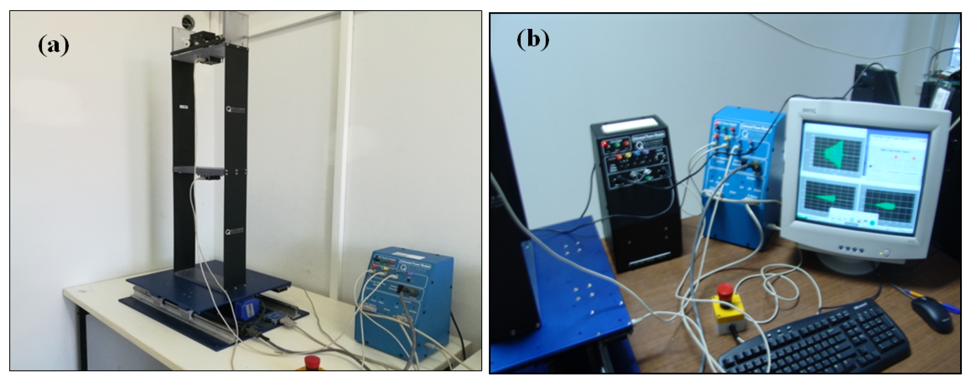
Figure 2.
View of steel benchmark structure and shake table.
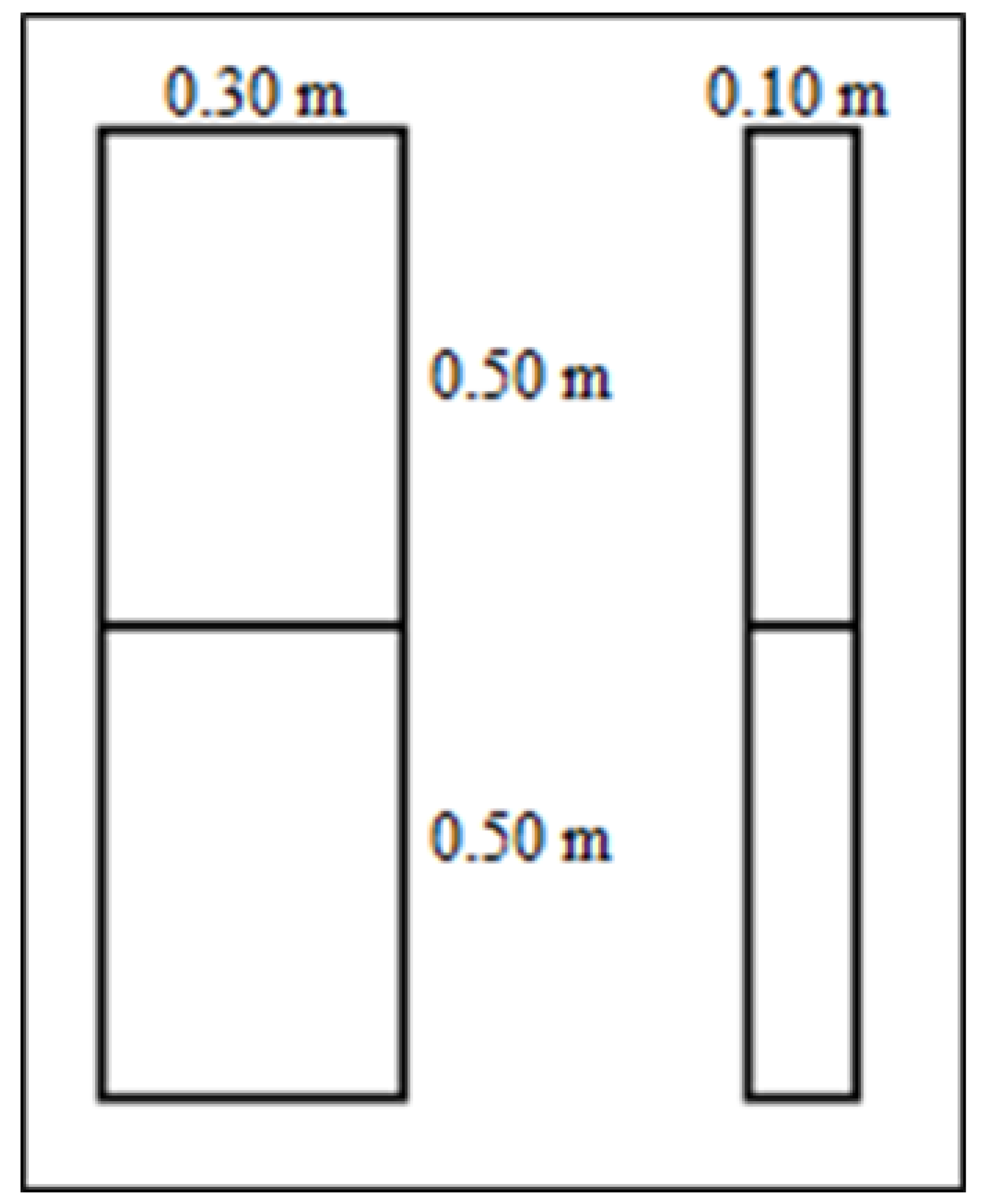
Figure 3.
Monthly average temperature changes in Samsun province of Turkey.
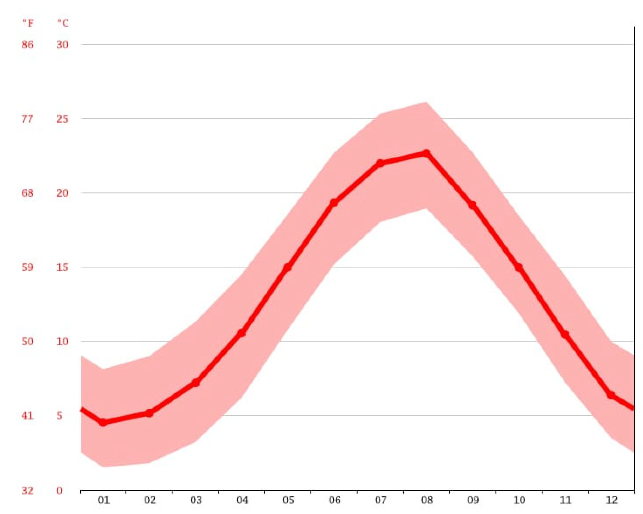
Figure 4.
Accelerometers location of experimental model in the 3D view a) Test layout for first measurement b) Test layout for second measurement.
Figure 4.
Accelerometers location of experimental model in the 3D view a) Test layout for first measurement b) Test layout for second measurement.
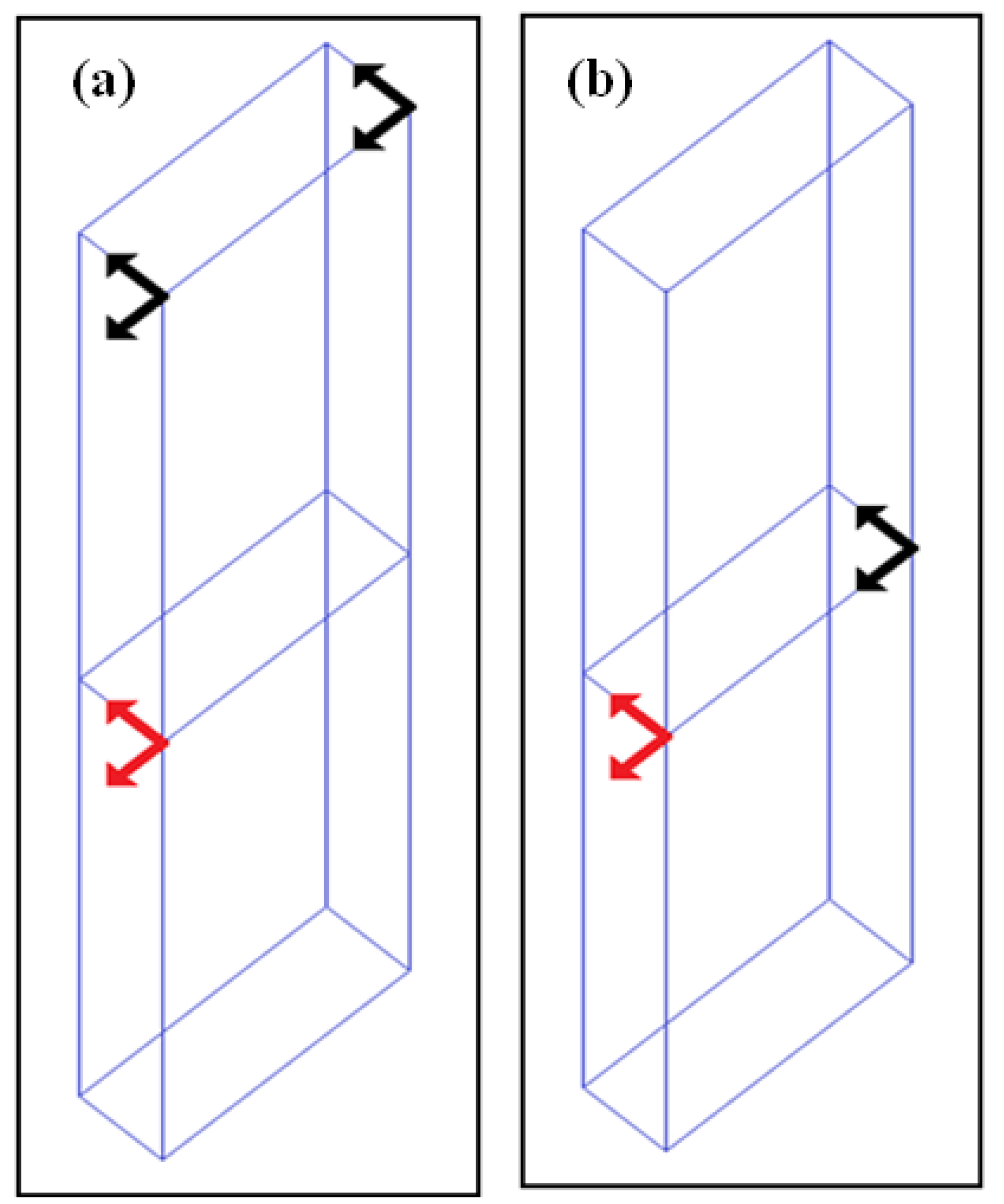
Figure 5.
a) Ambient vibrations recorded by the accelerometer b) Ambient excitation data from the recorded micro tremor data on ground level used in the shake table.
Figure 5.
a) Ambient vibrations recorded by the accelerometer b) Ambient excitation data from the recorded micro tremor data on ground level used in the shake table.
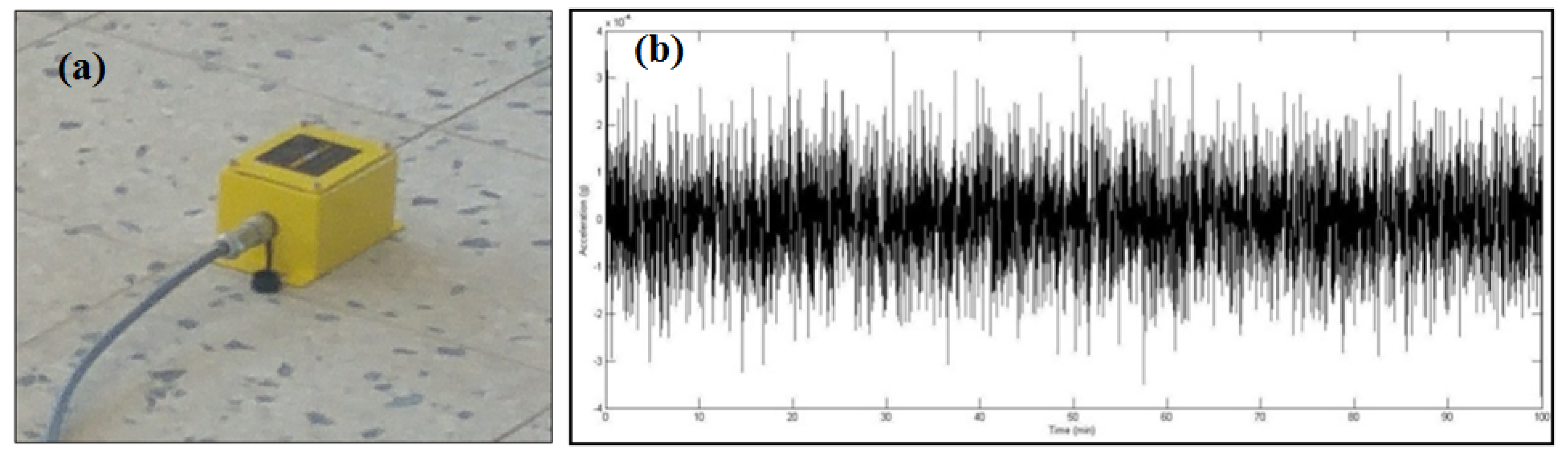
Figure 6.
Singular values of spectral density matrices at +2 °C
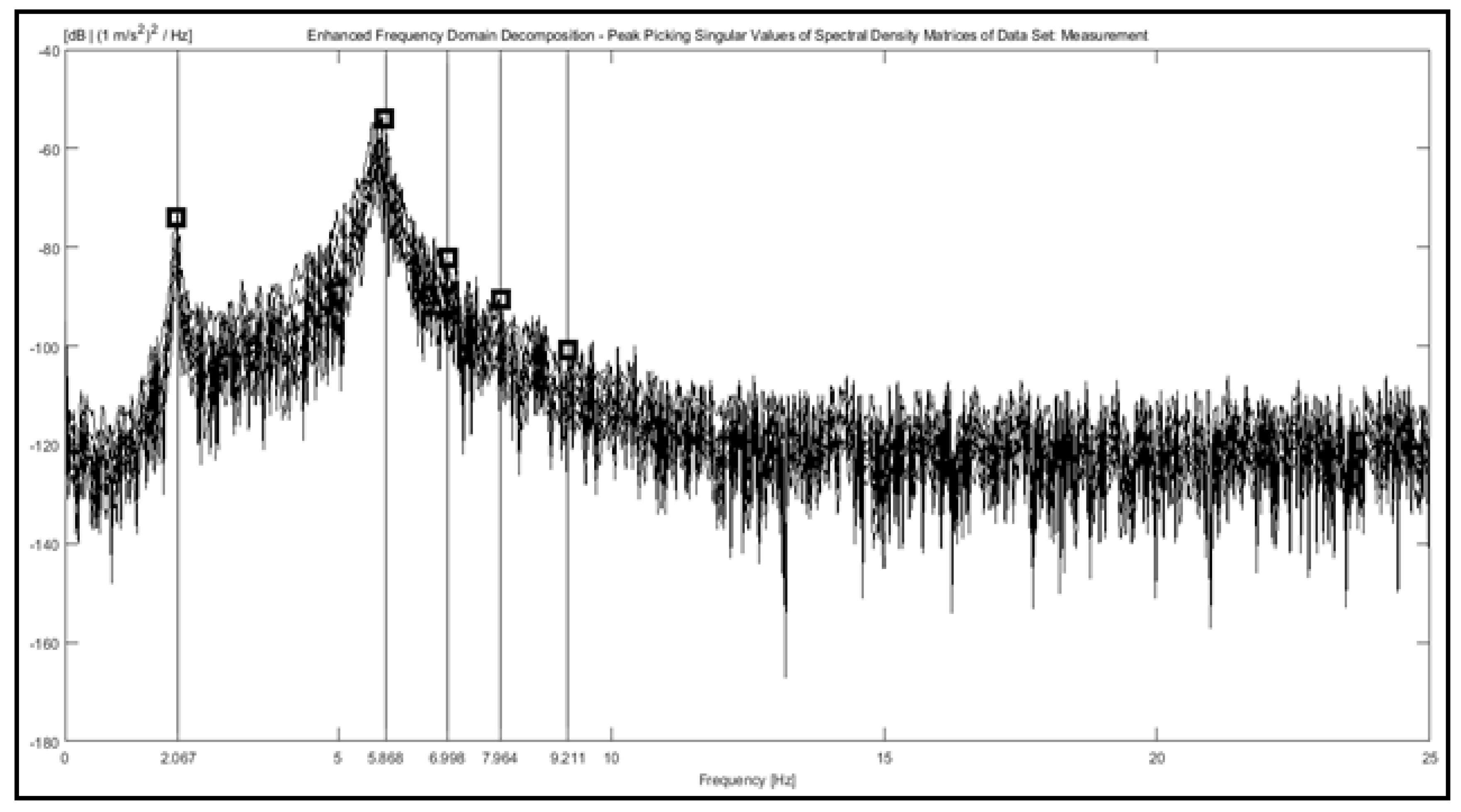
Figure 7.
Identified mode shapes of steel benchmark structure at +2 degrees a) 1st Mode Shape (f=2.067 Hz, ξ=0.672) b) 2nd Mode Shape (f=5.868 Hz, ξ=1.822) c) 3rd Mode Shape (f=6.998 Hz, ξ=1.035) d) 4th Mode Shape (f=7.964 Hz, ξ=0.551) e) 5th Mode Shape (f=9.211 Hz, ξ=0.670).
Figure 7.
Identified mode shapes of steel benchmark structure at +2 degrees a) 1st Mode Shape (f=2.067 Hz, ξ=0.672) b) 2nd Mode Shape (f=5.868 Hz, ξ=1.822) c) 3rd Mode Shape (f=6.998 Hz, ξ=1.035) d) 4th Mode Shape (f=7.964 Hz, ξ=0.551) e) 5th Mode Shape (f=9.211 Hz, ξ=0.670).
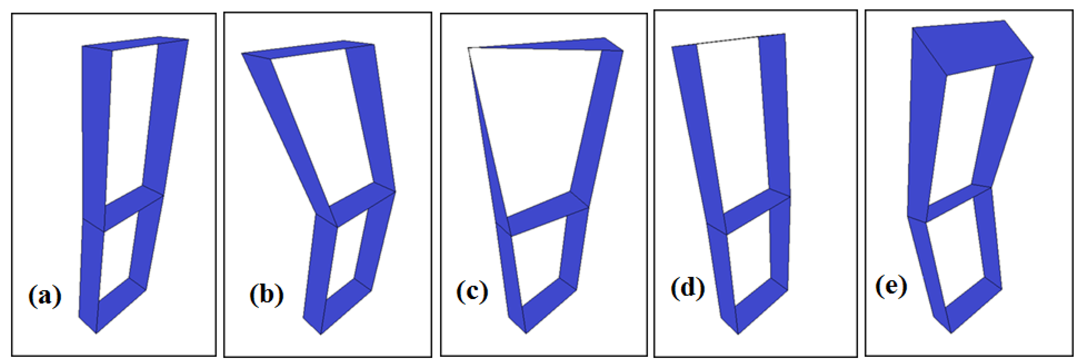
Figure 8.
Singular values of spectral density matrices at +32 °C
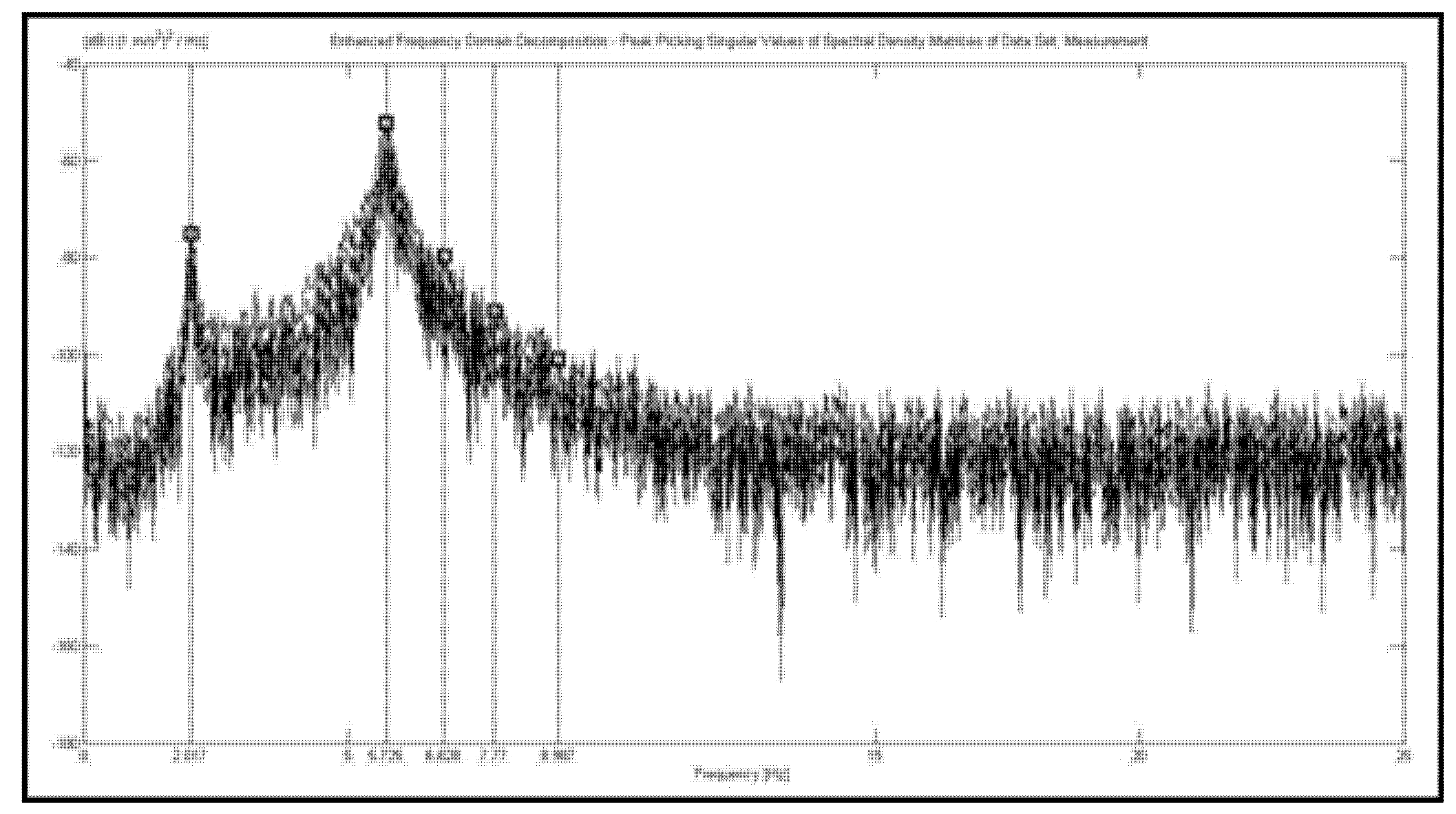
Figure 9.
Identified mode shapes of steel benchmark structure at +32 degrees a) 1st Mode Shape (f=2.017 Hz, ξ=0.672) b) 2nd Mode Shape (f=5.725 Hz, ξ=1.822) c) 3rd Mode Shape (f=6.828 Hz, ξ=1.035) d) 4th Mode Shape (f=7.770 Hz, ξ=0.551) e) 5th Mode Shape (f=8.987 Hz, ξ=0.670).
Figure 9.
Identified mode shapes of steel benchmark structure at +32 degrees a) 1st Mode Shape (f=2.017 Hz, ξ=0.672) b) 2nd Mode Shape (f=5.725 Hz, ξ=1.822) c) 3rd Mode Shape (f=6.828 Hz, ξ=1.035) d) 4th Mode Shape (f=7.770 Hz, ξ=0.551) e) 5th Mode Shape (f=8.987 Hz, ξ=0.670).
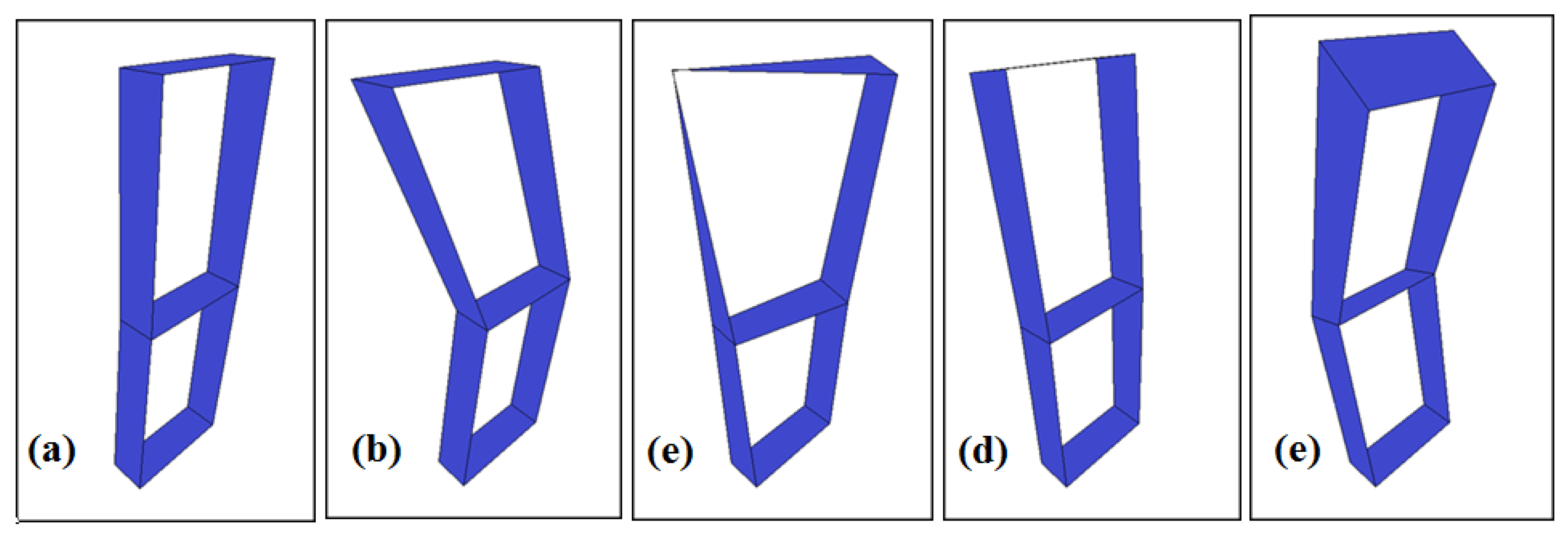
Table 1.
Shake Table Specifications.
| Dimensions (H x L x W) | (61 x 46 x 13) cm |
| Total mass | 27.2 kg |
| Payload area (L x W) | (46 x 46) cm |
| Maximum payload at 2.5 g | 7.5 kg |
| Maximum travel | ± 7.6 cm |
| Operational bandwidth | 10 Hz |
| Maximum velocity | 66.5 cm/s |
| Maximum acceleration | 2.5 g |
| Lead screw pitch | 1.27 cm/rev |
| Servomotor power | 400 W |
| Amplifier maximum continuous current | 12.5 A |
| Motor maximum torque | 7.82 N.m |
| Lead screw encoder resolution | 8192 counts/rev |
| Effective stage position resolution | 1.55 μm/count |
| Accelerometer range | ± 49 m/s² |
| Accelerometer sensitivity | 1.0 g/V |
Table 2.
Chemical composition of galvanized steel.
| C% | Si% | Mn% | P% | S% | Cr% | Mo% | Co% | Cu% | Nb% |
| 0,0402 | 0,0087 | 0,1691 | 0,0234 | 0,004 | 0,0123 | 0,005 | 0,01 | 0,0055 | 0,0021 |
| Ti% | V% | W% | Pb% | Zn% | Sn% | A1% | Sb% | Ni% | Fe% |
| 0,001 | 0,0277 | 0,01 | 0,005 | 0,001 | 0,0025 | 0,0194 | 0,005 | 0,0664 | 99,61 |
Table 3.
Experimental modal analysis result at the steel benchmark structure at +2.
| Mode number | 1 | 2 | 3 | 4 | 5 |
| Frequency (Hz) | 2.067 | 5.868 | 6.998 | 7.964 | 9.211 |
| Modal damping ratio (ξ) | 0.672 | 1.822 | 1.035 | 0.551 | 0.670 |
Disclaimer/Publisher’s Note: The statements, opinions and data contained in all publications are solely those of the individual author(s) and contributor(s) and not of MDPI and/or the editor(s). MDPI and/or the editor(s) disclaim responsibility for any injury to people or property resulting from any ideas, methods, instructions or products referred to in the content. |
© 2025 by the authors. Licensee MDPI, Basel, Switzerland. This article is an open access article distributed under the terms and conditions of the Creative Commons Attribution (CC BY) license (http://creativecommons.org/licenses/by/4.0/).
Copyright: This open access article is published under a Creative Commons CC BY 4.0 license, which permit the free download, distribution, and reuse, provided that the author and preprint are cited in any reuse.


