Submitted:
07 July 2025
Posted:
08 July 2025
You are already at the latest version
Abstract
The paper presents a comprehensive method for the elastodynamic analysis of mobile mechanical systems, based on the finite element method. Using Kane’s algorithm, which is employed in the dynamic analysis of mechanical systems with rigid bodies, a method is developed that, by superimposing the rigid body motion over the one of a deformable body, allows to identify the kinematic and dynamic components of the matrices involved in the motion equations namely, the mass matrix, stiffness matrix, damping matrix, and the force vector acting on the system. The method is applied to a high-speed mechanism used for actuating an internal combustion engine with three in-line pistons. Within this method, each kinematic link is considered as a finite element, with corresponding reference frames for which the kinematic and dynamic components of the matrices involved in the motion equations are determined. To solve the differential equations system, a modal superposition method is applied, which enables the decoupling of the equations and to identify the time-varying diagrams for nodal displacements, both longitudinal and transversal displacements, and consequently to determine the accelerations of the kinematic links, which are useful in vibration analysis. The strength force is considered the force exerted by the gas on the piston head, which was experimentally determined under laboratory conditions. The theoretical results obtained are validated through virtual prototyping and experimental tests.
Keywords:
finite element
; dynamic analysis
; deformable bodies
; vibration modes
; engine mechanism
; joint clearance
1. Introduction
The elastodynamic analysis of mobile mechanical systems is a highly debated research topic, especially in the context of the dynamics of mobile mechanical systems with elastic elements. Most of the research conducted among time, has aimed at accurately capturing the vibrations and flexibility of the components within the structure of the studied mechanisms, as well as experimentally validating these findings, as seen in [1,2].
The studies carried out on mobile mechanical systems have enabled the analysis of elastodynamic phenomena and vibrations under high-speed operating conditions. The use of the finite element method in the context of these analyses provides a detailed representation of deformations, fully integrated with the kinematic and dynamic models of the studied mechanisms. Furthermore, by complementing theoretical research with experimental validations for direct comparison with simulations and numerical processing, the obtained results have only increased the credibility and relevance of the research, as observed in [3,4].
Addressing to the elastodynamic analysis, and targeting mobile mechanical systems through an integrated concept of theoretical (mathematical) modeling – numerical processing – virtual prototyping – experimental validation, as exemplified in [5], these provides a classical methodological extensibility. This is compatible with formalisms such as Lagrange, Gibbs-Appell, and Hamilton, which, when combined with the finite element method or multibody dynamics, it generates modern research trends aimed at ensuring continuity in the field.
On the other hand, the studies presented in [6,7,8], which follow the aforementioned approach, are highly complex, as the use of the finite element method and the comparison of modal-dynamic analysis results, and these involves a large volume of numerical processing with high computation times, especially for extended models. Another particularly important aspect is the validation of the methods and tools, which are specific to the elastodynamic analysis. These were performed on only one mechanism, implying a limited validation. In this context, validating other mechanism configurations requires adapting the methods and newly validating the undertaken research.
If we consider the research in [9,10], which highlights measurement errors and inconsistencies in the obtained results, it becomes evident that experimental determinations are influenced by vibrations and the conditions under which experimental testing was conducted. Consequently, the results reveal incomplete alignments or discrepancies compared to the numerical processing of the mathematical models and, implicitly, with those obtained through virtual prototyping.
Moreover, the research in [10] also addresses to another highly important aspect in the dynamic behaviour of mobile mechanical systems, namely when the kinematic joints of a spatial mechanism exhibit a mechanical clearance. Thus, the analysis targets an advanced dynamic modelling of a spatial mechanism that includes impact forces and friction inside the joints, specifically adapted for microgravity conditions. As for the experimental analysis, it places greater emphasis on the joint clearance, which in microgravity can significantly degrade the mechanism motion accuracy. It is also noted that the methods used in the mechanism dynamic analysis have a limited applicability, and for generalizing them to be applied to more complex mechanisms, it requires substantial adaptations.
Similar to the studies presented in [10], the research in [11] also highlights several study methods applied to planar mechanisms, but with ambiguous experimental validation, which can only be certified through virtual prototyping.
It should be noted that a crucial influence on an elastodynamic analysis involving a mobile mechanical system is the dependence on the mechanical properties of the materials from which the system components are made. For this purpose, studies such as [12,13] have considered components made from materials with linear elasticity. However, the continuation of research in this direction also targets elastodynamic analyses of mobile mechanical systems with large component deformations or the use of materials with nonlinear mechanical properties, such as those described in [14,15,16].
In the research from [17], the authors develop a hybrid elastodynamic modelling, in which the mobile mechanical system is decomposed into substructures, some of them simulated numerically, others tested experimentally. The overall model of the mechanical system is then assembled using frequency-based substructuring methods. The aim of this research is to model the mechanical system in order to produce more realistic predictions regarding vibrations, system stability, and dynamic loads. Thus, the scientific approach involves a high methodological complexity through numerical modelling and experimental testing, which may lead to potential errors in the results and demands rigorous experimental procedures.
Therefore, the innovative aspect that ensures the continuity of research involving mobile mechanical systems elastodynamic analyses, lies in the development of mathematical models that also take into account the impact forces within joints where are present the potential deviations. These deviations significantly influence the quality of the results through which the system is rigorously validated, especially from an experimental viewpoint , as it can be seen in [18,19].
Considerring the research highlighted above and the weaknesses that an elastodynamic analysis of a mobile mechanical system may have, this paper aims to achieve the following objectives: Coupling the motion of a rigid body with one of a deformable body and identifying the static and dynamic components of the matrices in the equations of motion – interfacing the Kane method with the finite element method; Modal dynamic analysis through the modal superposition method with the nodal displacements identification; Elastodynamic analysis by determining displacements, velocities, and accelerations in deformable body motion; Developing mathematical models on a crank-connecting rod mechanism used to drive a three-cylinder inline internal combustion engine; Elastodynamic analysis of the mechanism using MSC Adams software and comparing the results with those obtained from mathematical model processing; Experimental analysis of the mechanism by monitoring the variation of the kinematic and dynamic parameters in both time and frequency domains.
These objectives are achieved according to the research workflow presented in Figure 1.
2. Mathematical Models for Dynamic Analysis of Mechanisms with Deformable Elements
There will be considered a kinematic linkage made of ,,n–1” solid–rigid, connected together through kinematic joints as it can be remarked in Figure 2. Thus, there will be accepted the solid “n” is a deformable solid.
The following notations will be introduced:
– is the reference coordinate system attached to the link “i” with versor base of ;
– is the global reference coordinate system with a versor base of;
– is the relative translational vector between ,,i” and ,,i–1”, depending on ,,Ri-1” tried, which exists, if between ,,i” and ,,i-1” links, there is a joint;
– position vector of the ,,O’i” point, expressed in the ,,Ri–1” reference coordinate system, when the relative translation begins.
Thus, the following equations can be written:
There will be introduced the transformation matrices for crossing from a reference coordinate system to another, by having in sight Equation (3).
Thus, the Equations (1) and (2) becomes:
By having in sight the Figure 3, onto En link, there will be considered the Mn point and u(M,t) displacement. The position vector of the P point is:
where: represents the coordinates transformation matrix.
The elastic displacement vector is:
where: – represents the form functions matrix or interpolating polynomial matrix; – is the nodal displacements vector.
Based on previous equations, there will be obtained:
There will be introduced the Equations (8) and (14) in Equation (6):
Thus, there will be considered the following generalized coordinates:
It will be obtained:
For the speeds calculus, there will be differentiated the (44) in raport with time :
Also, the Equation (14) it will be differentiated in raport with the time, and there will be obtained :
By reversing at the workflow with the use of matrices, we will differentiate the Equation (15), depending on time and we will obtain :
By taking into account the Equation (16), the Equation (20) becomes :
Also we will obtain the accelerations mathematical expression:
Based on the Equation (16), the Equation (22) becomes :
Thus, there will be elaborated the proper mathematical models for the motion equations in Kane formalism, for the holonomic case are [22]:
where: Q represents the generalized forces associated to the exterior loadings and connection forces; Q* represents the generalized forces associated to inertial torsors.
where: is the resultant force associated to Mk point; is the partial speed associated to speed of Mk point; is the resulted torque associated to the “i” kinematic element. is the partial angular speed, associated to the “i” element and to vr generalized speed.
For the “i” element, by taking into account the “q” nodal displacements, the generalized force associated to the inertial torsors, has the following form:
For the “i” element, it can be written:
The one from (29), by considering that the ω speed has small values, this it can be neglected.
From the (21) equation, it can be obtained:
Based on the Eqns (27) and (23), we will obtain the generalized forces attached to the inertial ones, as it follows:
The generalized force attached to the exterior forces, by supplementary considering the stiffness and dumping is:
The exterior forces and the exterior torque – T, which actuates on the considered element:
Thus, we consider the angular speed ω at small values and it will result: By considering the F – force actuates on the “n” element, it can be written:
The force resulted from the “n” element stiffness is:
where : [K] is the stiffness matrix, given by:
In (37), we identify: [B] is the connection matrix between deformations and displacements; [D] is the material properties matrix.
Thus, the force resulted from the dumping has the following form:
where: [C] is the dumping matrix given by:
where [μ] is the dumping coefficients matrix.
By turning at the Equation (24), which means: Q+Q*=0, and introducing the Equation (40) in (24) we obtain:
For a finite element “e” the motion is described by the following equation system:
From the Equation (41), we identify the terms coefficients , , namely , as it follows:
The mass matrix is:
The dumping matrix with both components, respectively static and dynamic is:
The elemental nodal force can be determined with the following relation:
The stiffness matrix with both components, respectively static and dynamic is:
3. Elastodynamic Analysis of the Mechanism from an Internal Combustion Engine
There will be analyzed, under kinematic and dynamic aspects, a mechanism from an internal combustion engine, shown in Figure 4. This mechanism consists of the following components: crankshaft 1, connecting rod 2, piston 3. The analyzed motion is transmitted from the crankshaft through connecting rods at the three in–line pistons. By knowing the functional role and the mechanism destination, it is well known the fact that the functional cycle involves rapid motions, with an accentuated dynamic character. Thus, it is necessary to develop a kinematic and kinetostatic calculus, which assumes the variation motion laws during the time for the kinematic parameters and the connection forces of the kinematic joints. The crankshaft rotational speed is 6000rpm.
The mechanism motion is monitored on a time interval equal to 0.04 seconds when the crankshaft develops two complete rotations.
Thus, by having in sight the rapid motions of the links that generate high inertial forces, there will be imposed a mechanism elastodynamic analysis. For this, the mechanism connecting rods is analyzed as deformable bodies.
For the inverse dynamic analysis processing, it is needed to know the crankshaft angular speed, which is ω=628.318 radians/second, crank slider length r= 40millimeters, connecting rod length l= 137 millimeters, mass characteristics of the mechanism links (m1= 0.952 kilograms, m2= 0.153 kilograms, and m3= 0.214 kilograms), and the gas pressure developed on the piston head. There will be determined the positions, speeds, and accelerations of A, and B characteristic points, respectively angular speed and angular acceleration of the AB connecting rod.
The force developed by the gas pressure onto the piston head is:
where: pg– gas pressure, established experimentally; Ap – piston head surface.
There were experimentally determined the gas pressure developed onto the piston head, depending on the crankshaft angle as can be observed in Figure 5.
In Figure 5, there are presented the main parameters variation of an internal combustion engine, depending on the crankshaft rotational angle (Crank Angle, deg). Thus, it can be remarked on the four distinctive phases of the engine stroke: intake, compression, power, and exhaust. The diagrams main elements reported in Figure 5 are as follows:
- Black curve (cylinder gas pressure): Two major peaks are visible, corresponding to successive combustion events. The maximum values exceed 90 bar, indicating the fuel expansion phase. During compression, pressure increases before ignition, followed by a rapid drop after the exhaust phase.
- Orange curve (fuel ignition): This shows the exact ignition point of the fuel, correlated with the peak pressure. A delay between injection and ignition is noticeable, which can be analyzed for optimizing engine performance.
- Green curve (reaction force in the piston, Fx): A sharp increase in force occurs at ignition, followed by a controlled decrease. This confirms that gas expansion generates a maximum force on the piston, influencing the mechanical power output.
- Red and blue curves (intake and exhaust valve lift): Intake valves (blue curve) open at the beginning of the intake stroke and close at its end. The exhaust valves (red curve) open at the end of the expansion stroke and remain open until the beginning of the intake stroke.
Also, in the superior part of Figure 5, the pressure variation diagram was developed onto the piston head, in bar as measuring unit, depending on the crankshaft rotational angle. According to the Figure 5, it was obtained the force developed by the gas pressure, by knowing the piston head surface, and this variation was adapted as a function of time represented in Figure 6. Thus, the mechanism was modeled through beam elements type, as it can be seen in Figure 7 and Figure 8.
Each mechanism kinematic link will be considered as two finite elements, beam type, with two nodes at each end, respectively 3DoF for each node (Figure 9 and Figure 10). As loads, there were considered the finite elements weights and the force developed by the gas pressure onto the piston head, namely Fb. For finite element no. 2, the piston component can be replaced with a concentrated mass – mc.
The mechanical system motion can be reported at the following reference systems:
- R1(x1,y1,z1) – mobile reference system attached to the finite element no. 1;
- R2(x2,y2,z2) – mobile reference system attached to the finite element no. 2;
- R0(X0,Y0,Z0) – global reference system.
The proper mathematical model for ,,e’’ finite element displacements is:
where: – axial displacements; ,– transversal displacements and angular displacements. From Equation (48), it can be identified:
– is the interpolation functions matrix;
– is the nodal displacements vector for a finite element,,e “ with e=1,2– finite elements.
In this vector structure it will have axial and transversal displacements, as follows:
For the axial displacements, there will be adopted the linear interpolating model, and the form function matrix components become:
For the transversal displacements there will be adopted the cubic interpolating model, and the form function matrix components will be:
For the mechanism assembled structure will have:
– nodal displacements vector in the local coordinates system.
The motion equations, in a matrix form for the mechanism, are:
where:
– mass matrix, assembled for the entire analyzed mechanical system; – assembled stiffness matrix; – assembled dumping matrix; – nodal force vector, assembled for the entire mechanical system.
For the presented mechanical system, made of two finite elements (beam type) with 3DoF on each node, there will be determined the matrices from the motion equations structure.
3.1. Nodal Force Calculus
The nodal forces corresponding to the local coordinates system will be obtained by having in sight the Equation (45). Thus, the nodal force for the ,,e” finite element can be determined with the following relations:
– static components:
– dynamic components:
Finite element no.1:
The nodal force static component, which corresponds to finite element no. 1, is:
where:
– material density; g – gravitational acceleration; – transversal section of the finite element „e” with e=1..2
The nodal force static component expressed by taking into account the local reference system is:
The nodal force dynamic component is:
The angular speed can be written as a anti-symmetrical matrix as follows:
The force which actuates on the finite element no. 1, in the local reference system is:
where: – is the transformation matrix of the coordinates for crossing from a reference system attached to finite element „e”, to a global reference system (e=1,2):
The force that actuates onto finite element no. 1 in the global reference system is:
where: – is the coordinates transformation matrix, for crossing from a reference system attached to finite element no. 1, to the global reference system.
Finite element no. 2:
The static components can be obtained in accordance with the global reference system by considering the nodal mass force as:
where: N2 – is the form functions matrix which corresponds to the finite element no. 2.
The nodal force static component, depending on the local reference system is:
The produced force by the gas pressure in the local reference system, which actuates in node no. 3, is given by:
The dynamic components are:
where:
Is the B point vector in the local coordinates system, namely R2(x2,y2,z2):
Is the generalized coordinates vector for the finite element no. 2 (mass center position and finite element no. 2 orientation):
Is the vector of generalized speeds:
Is the vector of generalized accelerations:
Point C2 position is:
Point C2 speed is:
Point C2 acceleration is:
The angular speed of the finite element “i” is:
The angular acceleration of the finite element “i” is:
The coordinates transformation matrix for crossing from a local axis reference system Ri(xi,yi,zi) to a global reference system R0(X0,Y0,Z0) is:
Thus, in this case, the coordinates transformation matrix for crossing from a local axis reference system R1(x1,y1,z1) to a global reference system R2(x2,y2,z2) is:
The force which actuates on the finite element no. 2, in the local axis system is:
The force which actuates on the finite element no. 2, in the global axis system is:
where: – is the coordinates transformation matrix, for crossing from a reference system attached to finite element no. 1, to a global reference system.
The assembled nodal force for the engine mechanism, according to the global reference system, is:
3.2. Stiffness Matrix
where: – represents the static component; – represents the dynamic component; – material elasticity modulus.
Finite element no. 1:
Static component. The stiffness matrix in a local coordinate system is:
where: – for transversal displacements; for axial displacements.
The stiffness matrix for the transversal displacements:
The stiffness matrix for the axial displacements:
Dynamic component: For the finite element no. 1, in the local axis reference system:
The stiffness matrix for the finite element no. 1, according to the local reference system is:
The stiffness matrix for the finite element no. 1, according to the global reference system is:
Finite element no. 2:
The static component of the stiffness matrix in the local axis reference system is:
The stiffness matrix which corresponds to transversal displacements is:
The stiffness matrix which corresponds to axial displacements is:
The assembled stiffness matrix for the finite element no. 2, according to the local reference axis system:
The dynamic component of the stiffness matrix in a local axis reference system is:
The stiffness matrix for the finite element no. 2, according to the local reference system is:
The stiffness matrix for the finite element no. 2, according to the global reference system is:
3.3. Mass Matrix
The mass matrix in the local coordinates system, can be written as follows:
where: – ,,e” finite element mass; – form function matrix (interpolating ones).
Finite element no. 1:
Finite element no. 2:
where: mp is the piston mass.
The piston was considered a concentrated mass, which was attached to the finite element no. 2, respectively in node no. 3.
The mass matrix in a global coordinates system is:
Finite element no. 1:
Finite element no. 2:
The equilibrium equation expressed in the local coordinates system has the following form:
Also: – are the nodal displacements in the global coordinates system; – represent the nodal forces in a global coordinates system.
The assembled equilibrium equations, in a global coordinates system have the following form:
where: – is the assembled stiffness matrix; – is the assembled nodal displacements vector; – represents the assembled nodal forces vector.
3.4. The Assembly of the Equations and Introducing the Contour Conditions
There will be introduced contour conditions (node no. 1 has a single DoF, which allows only the Q3 rotation, and node no. 3, has two DoFs which for this was canceled the Q8 displacement):
Finite element no. 1:
Finite element no. 2:
By considering the contour conditions, from the assembled matrix which interact in the motion equation, respectively, there will be canceled line 1, column 1, line 2, column 2, and line 8, column 8. Thus, in these conditions, the remaining matrices will have 6x6 dimensions.
The reduced mass matrix has the following form:
The reduced stiffness matrix has the following form:
The nodal force assembled for the considered engine mechanism, by having in sight the global reference system, is:
The elastic displacements vector for the element no. 1 is:
The elastic displacements vector for the element no. 2 has the following form:
or:
where:
The nodal displacements vector for the finite element no. 1, in the global reference system, is:
where: Q1=0; Q2=0 (by introducing the contour conditions).
The nodal displacement vector for the finite element no. 2, in the global reference system has the following form:
where: Q7=0, (by introducing the contour conditions).
3.5. Modal Dynamic Analysis
The motion equations are:
The motion equations, without dumping, are:
The solution of the differential Equation (121), where the coefficients are considered constant ones, has the following form:
By differentiating the above equation will be obtained:
The differential equation without dumping and external loads will be:
There will be obtained:
This is a proper value problem for the matrix .
For a system with ,,n” degrees of freedom we have ,,n” proper values ,,λ” and ,,n” proper vector sets .
For each ,,j” we have:
where: = is the natural circular frequency:
natural frequency:
There are proper vectors which represent the vibration modes, respectively the assumed structure form when this vibrates with a frequency of and which satisfies the equation:
For solving the motion equations system (120), there will be used the nodal superposition method. This method allows the user to detach the motion equations through a linear transformation as follows:
where: is the modal form coordinate which represents the ,,i” mass position in a ,,j” module; is the generalized coordinate which represents the ,,j” module response during time; depends on the position, not on the time; depends on time, and not on the position.
Under a matrix form:
where: modal matrix, where the modal forms will be written in columns.
We accept that the modal forms vector is orthogonal in rapport with the mass matrix, which means:
We reconsider the equation:
We differentiate twice the mathematical expression:
We introduce (137) in (136):
We multiply on the left side of the (138) relation with the term and taking into account the (135), there will be obtained:
The (132) relation, can be written as:
In the mathematical expression (140) we multiply on the left side with, and taking into account the (135), we will obtain:
where:
We introduce (141) in (139) and we will obtain:
The (143) mathematical expression represents the uncoupled differential equation set which are independent ones. Thus, the modal frequencies will be:
The natural frequencies are:
where: f1= 4,957487532Hz; f2= 542,9548523Hz; f3= 156,8132854Hz; f4= 3230,572390Hz; f5= 978,5360786Hz; f6= 93,29474415Hz.
We reconsider the following equation:
where: is the modal matrix form:
Based on numerical processing, there will be obtained the diagrams reported in Figure 11, Figure 12, Figure 13, Figure 14, Figure 15 and Figure 16, where it can be identify six proper vibration modes of the analyzed mechanism.
The generalized coordinates vector is:
This vector corresponds to the accelerations vector, which has the following form:
The force vector will be:
By solving the differential equations system (189), the equation system solution (121), is:
where - represents the nodal displacements. The elastic displacements can be obtained by solving the equation system:
3.6. Results of Numerical Processing
For the numerical processing of the mathematical models, a program was developed in the Maple programming environment, which allows simultaneous inverse dynamic analysis—when the elements of the mechanism are rigid bodies—as well as elastodynamic and modal dynamic analysis when the elements are deformable bodies.
Virtual prototyping involved building a 3D model of the engine mechanism. An interface was created for importing this model into the virtual environment of the MSC Adams software.
In the first stage, a numerical simulation of the mechanism kinematic model was performed, with the crankshaft rotation speed (6000 [rpm]) as input data, along with the geometric characteristics, mass properties of the mechanism’s kinematic links, and the local reference systems attached to the considered links and kinematic joints. The mechanism motion was studied over a time interval of 0.04 seconds when the engine crankshaft performed four complete rotations.
In the second stage, the dynamic model was developed, in which the gas pressure applied on the piston head is known, along with the geometry, material characteristics, and inertial properties of the kinematic links.
The torque variation law acting on the crankshaft was determined, and consequently, the engine crankshaft angular speed variation.
The pressure developed by the gas on the piston head was experimentally determined, and its variation, as a function of the crankshaft rotation angle, was shown in Figure 5.
In order to determine the crankshaft torque (engine torque), a function was created that enables the interface with the ADAMS programming environment, as follows:
Mm = M0 *(1-WX(MARKER_I, MARKER_J, MARKER_J)/ω0)
Where: Mm is the engine torque; M0 is the initial torque; ω0 is the initial angular speed; WX(MARKER_I, MARKER_J is the X-axis component corresponding to the crankshaft angular speed, between marker I and marker J, measured in accordance with the coordinate system attached to marker J.
For the analyzed case study, the torque function is given by:
Mm = -170000*(1-WX(MARKER_1,MARKER_2,MARKER_2)/100)
Figure 17 represents snapshots from the virtual simulation carried out using the Adams software.
The three connecting rods were analyzed as deformable bodies, with the transformation from rigid to deformable bodies being based on the finite element method.
The connecting rod linear and angular deformations were determined in the Adams programming environment, based on the theory developed by Craig & Bampton [23]. The results were compared with those obtained from the processing of the mathematical models in the modal dynamic analysis, as it can be remarked in Figure 18, Figure 19, Figure 20, Figure 21 and Figure 22.
4. Experimental Analysis
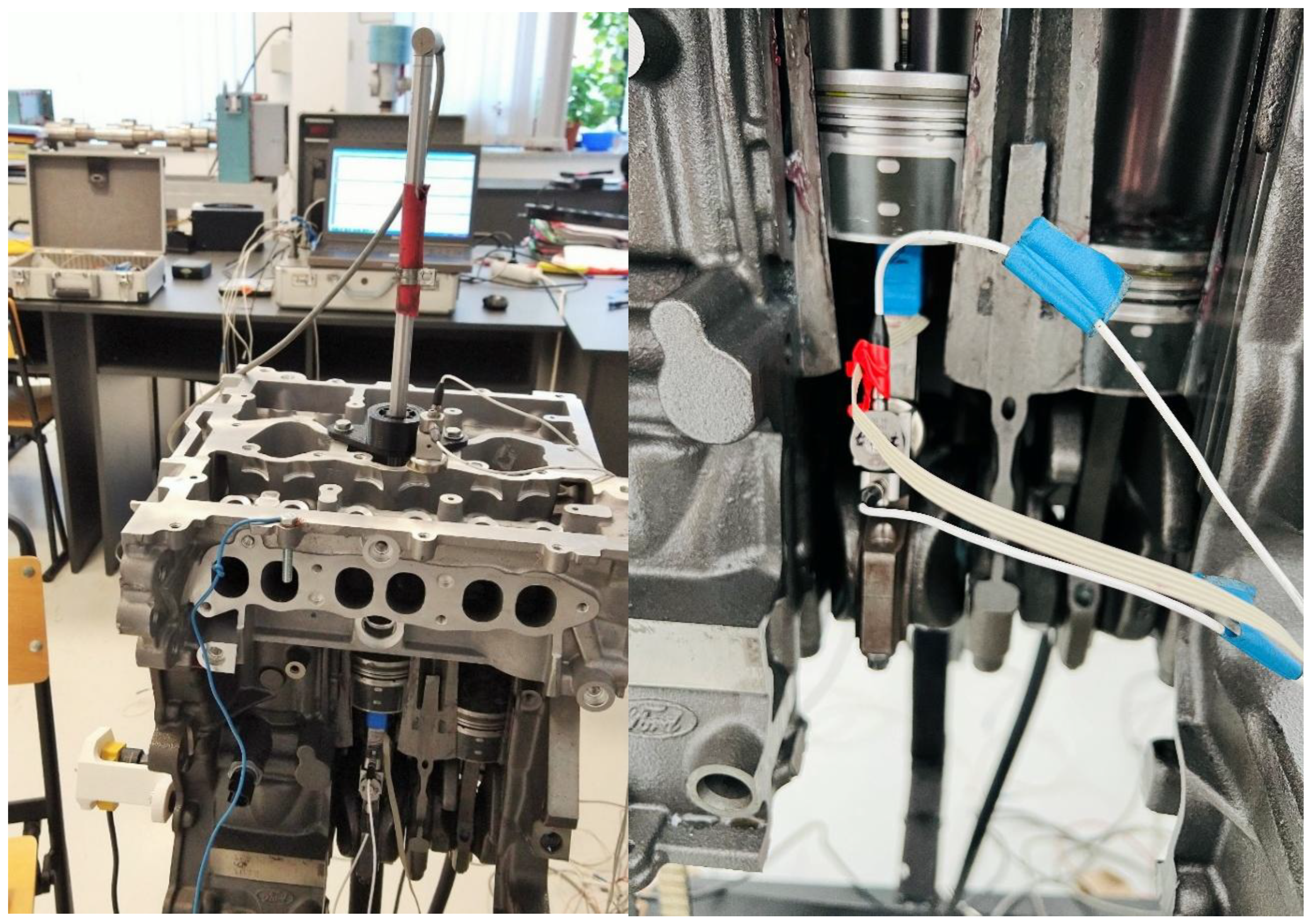
To determine the piston stroke, an HBK WA-L type inductive displacement transducer was used, mounted in an opening made in the engine cylinder head. This transducer is attached to the piston and allows precise measurement of its stroke during the mechanism functionality.
For piston stroke measurement, it was used an inductive displacement transducer type HBK WA-L, mounted an fixed through a hole especially created in the engine cylinder head. This transducer has the mobile component fixed to the piston and allow the user to measure with a high fidelity the piston displacement during engine mechanism functionality.
The transducers’ characteristics are the following:
- Transducer type: Inductive, linear;
- High precision: Compatible with dynamic measurements;
- Variable measuring domain: Selected for covering the entire piston stroke;
- Rigid coupling: This assures a measurement without mechanical interferences.
This transducer is used to analyze the piston kinematics, providing experimental data for validating the theoretical models and the virtual simulations performed in MSC ADAMS.
By using a precision transducer, it is possible to compare the experimental results with the predictions obtained through numerical modeling, thus ensuring the validity of the data and identifying deviations from the impact theory applied in the simulations.
For the mechanism dynamic analysis, there were used piezoelectric acceleration transducers, mounted on the connecting rod and the cylinder head for measuring longitudinal and transversal accelerations.
The configuration of the experimental setup:
- The connecting rod accelerometers were attached by using magnets to the flat surface of the connecting rod, near the strain gauge areas, to ensure accurate measurement of longitudinal and transversal acceleration.
- The cylinder head accelerometers were mounted above the analyzed piston, capturing the vibrations and accelerations transmitted through the engine.
The accelerometer characteristics are as follows:
- Type: Piezoelectric;
- Measurement range: ±50 g;
- Sensitivity: 10 mV/g
- Mounting method: Magnets for the connecting rod, screws for the cylinder head;
- Frequency domain: 0.5 Hz – 10 kHz
The purposes of using the mentioned accelerometers are:
- To determine the vibrations induced during the connecting rod and piston motions.
- To compare the accelerations simulated in MSC.ADAMS with those experimentally measured.
- To validate the dynamic model through frequency spectrum analysis of the measured accelerations.
By using these accelerometers, valuable data were obtained on the system’s dynamic behavior, allowing for an accurate correlation between simulations and experimental measurements. The following parameters were recorded:
-AccBiela_L(m/s2) – connecting rod longitudinal acceleration;
-AccBiela_T(m/s2) – connecting rod transversal acceleration;
-AccBloc_V(m/s2) – cylinder head vertical acceleration;
-AccBloc_T(m/s2) – cylinder head transversal acceleration;
-CursaPiston(mm) – piston stroke;
-FortaBiele(N) – connecting rod longitudinal force.
For a single connecting rod setup, experimental tests were carried out successively at three different excitation frequencies. The electric motor’s operating frequency was adjusted using a frequency converter, with values around: 0.7 Hertz, 1 Hertz, and 1.3 Hertz.
For each excitation frequency, the operating time was approximately 30 seconds in order to allow for a frequency analysis over a reasonably wide bandwidth. It is important to note that the frequency resolution is inversely proportional to the analysis signal length:
Df=1/Dt
Considering the relation (194), in the frequency analyses performed, the frequency displayed on the screen represents the center of the frequency band, while the actual frequency lies within that band. For this reason, it was preferred that the excitation frequency of the piston be calculated from the time-domain representations as the inverse of the piston stroke period.
The experimental recordings were carried out using the LAN-XI data acquisition system, model 3053-B120, manufactured by Brüel & Kjær, along with the Pulse Labshop software from the same manufacturer.
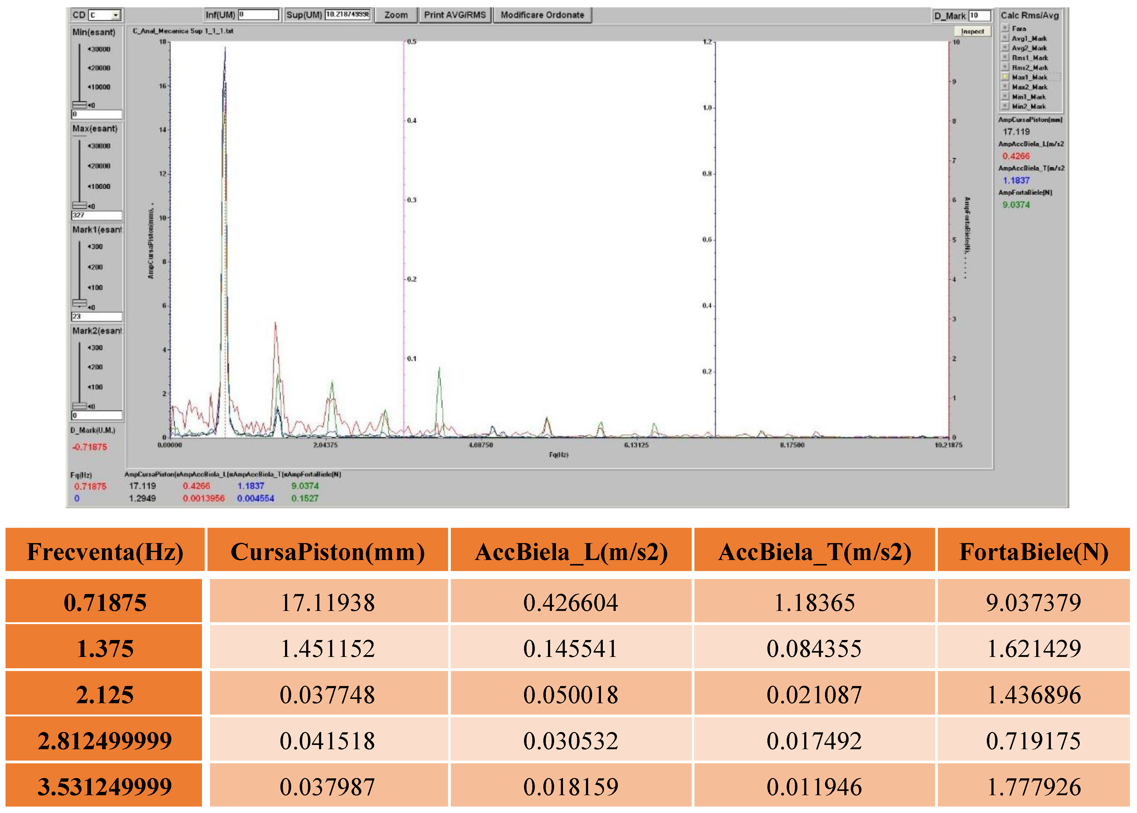
Post-processing analyses were performed using the Pulse Reflex and TestPoint software packages, which complement each other, and results of these are shown in Figure 30 and Figure 31.
Figure 29.
Experimental test rig for the dynamic analysis of the engine mechanism: Detailed view for the dynamic experimental analysis of the piston – connecting rod mechanism.
Figure 29.
Experimental test rig for the dynamic analysis of the engine mechanism: Detailed view for the dynamic experimental analysis of the piston – connecting rod mechanism.
For the connecting rod, as it can be remarked in Figure 30, the accelerations predominantly exhibit a sinusoidal pattern, with two impact zones occurring on either side of the piston stroke’s peak moment, corresponding to the points where the direction of the force acting through the connecting rod changes on the two lateral faces of the piston.
From the time-domain analysis of the connecting rod vibrations, it is observed that the longitudinal and transversal accelerations predominantly exhibit a sinusoidal pattern, with two impact zones on either side of the maximum point of the piston stroke. These correspond to the moments when the direction of the force transmitted by the connecting rod changes to the two lateral faces of the piston, as it can be remarked Figure 31.
The longitudinal force in the connecting rod shows inflection points at the maximum and minimum points of the piston stroke. These inflection points should be clearly delimited in the case of a connecting rod without clearances in the joints.
5. Conclusions
The dynamic response of the multibody system consists of two segments: one due to the initial conditions, which damps out quickly, and one due to the disturbing forces.
By applying the finite element method, the continuous system was replaced with a discrete system with a finite number of degrees of freedom. The problem unknowns are no longer displacement functions u(x,y,z,t), but rather the nodal displacements q(t).
The system of partial differential equations (the Lame equations from elasticity theory) is transformed into a system of differential equations. The matrices involved in the general equation of motion were identified based on the idea of superimposing rigid body motion over deformable body motion. The rigid body motion was defined by a set of reference coordinates that define the location and orientation of the local reference system of each kinematic link.
By eliminating the rigid body motion, a system of linear differential equations is obtained, this being clearly evidentiate due to the assumptions made, which include: the small deformations hypothesis; the small displacements hypothesis; the linear material hypothesis (Hooke law).
Also, assuming that the damping force is proportional to the velocity, we consider a system of linear differential equations with constant coefficients ([M], [K], and [C]).
By combining the two motions, a complete dynamic analysis is proposed with multiple applications in multibody system dynamics. The elastodynamic analysis involves two stages: the analytical determination of natural frequencies and vibration modes, and the determination of kinematic parameters in the deformable body motion of the kinematic links.
The mathematical models obtained for the multibody systems elastodynamic analysis were applied to a crank-connecting rod mechanism used to drive a three-piston in-line engine. Each kinematic link was considered as a finite element “beam” type, with two nodes and three degrees of freedom per node, corresponding to the nodal displacements vector. The shape function matrices for axial and transversal displacements, as well as the generalized coordinate vector for the entire assembled system, were determined. For each finite element, the nodal force static and dynamic components, the stiffness matrix, and the damping matrix were determined relative to the local axis system and the global axis system, using coordinate transformation matrices when moving from one reference system to another. This was possible by superimposing rigid body motion with elastic solid motion, using Kane’s algorithm [22].
Using the modal superposition method, there were determined the linear, transversal, and angular nodal displacements for the connecting rod of the mechanism.
Thus, by using the finite element method, the variation of longitudinal and transversal elastic displacements in 3D format was obtained along with the entire length of the connecting rod, and in a 2D format at different points in the connecting rod plane.
In order to verify the results obtained from the processing of the mathematical models, a dynamic analysis was performed in the Adams programming environment based on multibody system dynamic theory.
The system’s motion is driven by the force developed by the gas on the piston head as a result of the gas pressure which was experimentally determined. The same force was considered in the mathematical models.
A comparative analysis was performed for the linear, transversal, and angular nodal displacements, where it was observed that the maximum and minimum values are close, including the shape of the variation curves.
From the 3D diagrams, it is observed that the maximum value of the longitudinal elastic displacements is 0.003 millimeters, while the transversal elastic displacements reach a value of 0.015 millimeters.
At the midpoint of the connecting rod length, the variation curves for the two types of longitudinal and transversal displacements register the same extreme values with similar variation shapes. The recorded differences mainly occur due to the fact that in the dynamic analysis with the Adams program, the engine torque exhibits a jump during startup over a period of a few milliseconds, then stabilizes around 150 [Nm].
The matrix approach to the mathematical models allowed the development of a flexible calculation program with rapid applications for the dynamic analysis of multibody systems with deformable elements.
The experimental analysis enabled the time and frequency monitoring of kinematic and dynamic parameters, mainly for each of the three connecting rods of the mechanism (forces, longitudinal, and transversal accelerations). The dynamic response monitoring of the three connecting rods was performed at lower speeds and without load on the piston, on a longitudinally sectioned engine.
Author Contributions
Conceptualization, N.D. and S.D.; methodology, N.D.; software, A.S.R.; validation, N.D., S.D. and C.C.; formal analysis, C.C.; investigation, N.D.; resources, S.D.; data curation, A.S.R.; writing—original draft preparation, N.D.; writing—review and editing, C.C.; visualization, A.S.R.; supervision, N.D.; project administration, N.D.; funding acquisition, S.D. All authors have read and agreed to the published version of the manuscript. All authors have read and agreed to the published version of the manuscript.
Funding
Not applicable.
Data Availability Statement
Data available on request to the authors.
Acknowledgments
Not applicable.
Conflicts of Interest
The authors declare no conflicts of interests.
References
- Piras, G.; Cleghorn, W.L.; Mills, J.K. Dynamic finite-element analysis of a planar high-speed, high-precision parallel manipulator with flexible links. Mech. Mach. Theory. 2005, 40, 849–862. [Google Scholar]
- Cleghorn, W.L.; Fenton, G.; Tabarrok, B. Finite element analysis of high-speed flexible mechanisms. Mech. Mach. Theory. 1981, 16, 407–424. [Google Scholar]
- Bahgat, B.M.; Willmert, K.D. Finite element vibrational analysis of planar mechanisms. Mech. Mach. Theory. 1976, 11, 47–71. [Google Scholar]
- Rong, B.; Rui, X.T.; Tao, L.; Wang, G.P. Theoretical modeling and numerical solution methods for flexible multibody system dynamics. Nonlinear Dyn. 2019, 98, 1519–1553. [Google Scholar]
- Song, Ji Oh; Haug, J. Dynamic analysis of planar flexible mechanisms. Computer Methods in Applied Mechanics and Engineering. 1980, 24, 359–381. [Google Scholar]
- Vlase, S.; Marin, M.; Itu, C. Gibbs–Appell Equations in Finite Element Analysis of Mechanical Systems with Elements Having Micro-Structure and Voids. Mathematics, 2024, 12, 178. [Google Scholar] [CrossRef]
- Scutaru, M.L.; Vlase, S. Two-Dimensional Equivalent Models in the Analysis of a Multibody Elastic System Using the Finite Element Analysis. Mathematics 2023, 11, 4149. [Google Scholar] [CrossRef]
- Korayem, M.H.; Dehkordi, S.F. Motion equations of cooperative multi flexible mobile manipulator via recursive Gibbs-Appell formulation. Appl. Math. Model. 2019, 65, 443–463. [Google Scholar]
- Wang, Z.; Tian, Q.; Hu, H. Dynamics of Flexible Multibody Systems With Hybrid Uncertain Parameters. Mech. Mach. Theory. 2018, 121, 128–147. [Google Scholar]
- Ren, J.; Zhang, J.; Wei, Q. Dynamic analysis of planar four-bar mechanism with clearance in microgravity environment. Non-linear Dyn. 2024, 112, 15933–15951. [Google Scholar] [CrossRef]
- Marques, F. , Roupa, I., Silva, M.T., Flores, P., Lankarani, H.M. Examination and comparison of different methods to model closed loop kinematic chains using Lagrangian formulation with cut joint, clearance joint constraint and elastic joint approaches. Mech. Mach. Theory. 2021, 160, 104294. [Google Scholar]
- Zhang, X.; Erdman, A.G. Dynamic responses of flexible linkage mechanisms with viscoelastic constrained layer damping treat-ment. Comput. Struct. 2001, 79, 1265–1274. [Google Scholar]
- Xianmi, Z.; Yunwen, S. Optimal design of flexible mechanisms with frequency constraints. Mech. Mach. Theory. 1995, 30, 131–139. [Google Scholar]
- Shabana, A.A. On the integration of large deformation finite element and multibody system algorithms. In Proceedings of the International Conference on Mechanical Engineering and Mechanics, Halkidiki, Greece, 12–17 June 2005; 1–2; pp. 63–70. [Google Scholar]
- Luo, K.; Liu, C.; Hu, H.Y. Nonlinear static and dynamic analysis of hyper-elastic thin shells via the absolute nodal coordinate formulation. Nonlinear Dyn. 2016, 85, 949–971. [Google Scholar]
- Lu, H.J.; Rui, X.T.; Ding, Y.Y.; Chang, Y.; Chen, Y.H.; Ding, J.G.; Zhang, X.P. A hybrid numerical method for vibration analysis of linear multibody systems with flexible components. Appl. Math. Model. 2022, 101, 748–771. [Google Scholar]
- Wei Ma, Haitao Liu, Guofeng Wang, Juliang Xiao. An elastodynamic modeling approach based on experimental substructuring for a mobile hybrid robot. Mech. Mach. Theory. 2025, Elsevier, Vol. 205.
- Song, N. , Peng, H., Xu, X., Wang, G.: Modeling and simulation of a planar rigid multibody system with multiple revolute clearance joints based on variational inequality. Mech. Mach. Theory. 2020, 154, 104053. [Google Scholar]
- Sun, D., Shi, Y., and Zhang, B. Dynamic Analysis of Planar Mechanisms With Fuzzy Joint Clearance and Random Geometry. ASME. J. Mech. Des. 2019; 141: 042301. [CrossRef]
- Dumitru, N., Craciunoiu, N., Geonea, I., Copilusi, C. Elastodynamic analysis of a mechanism with flexible links. Proceedings of the World Congress on Engineering,Vol. 2,WCE- 2017. London U.K. 5-7 June 2017. 821 – 828.
- Amirouche, F. Computational methods in multibody dynamics, Prentice-Hall; US; 1992.
- Kane, T.; Likins, P.; Levinson, D.; Spacecraft Dynamics, Mc. Graw-Hill; US; 1983.
- Craig Jr, R. R.; Bampton, M. C. Coupling of substructures for dynamic analyses. AIAA journal. 1968, 6, 1313–1319. [Google Scholar]
Figure 1.
Research workflow.
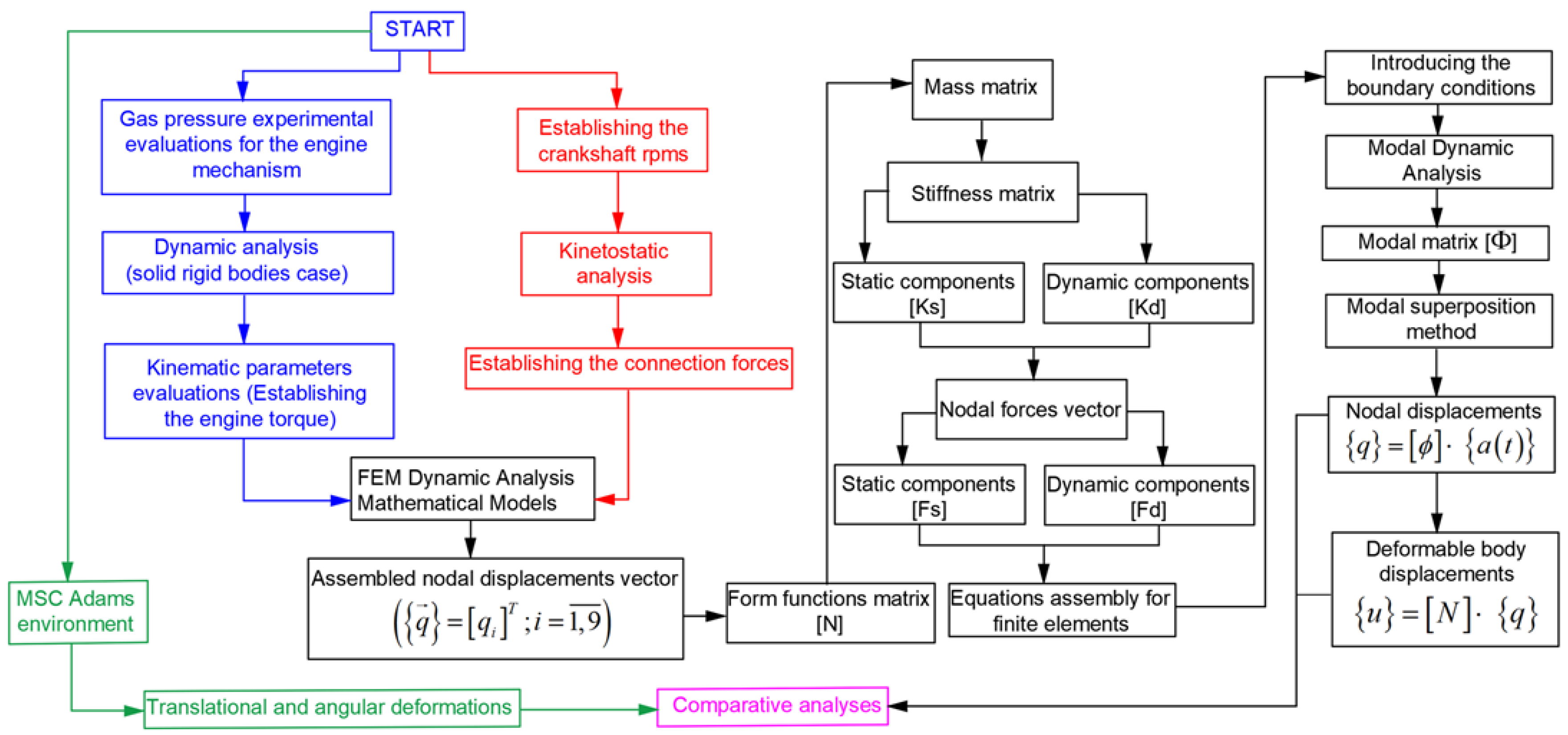
Figure 2.
General kinematic model.
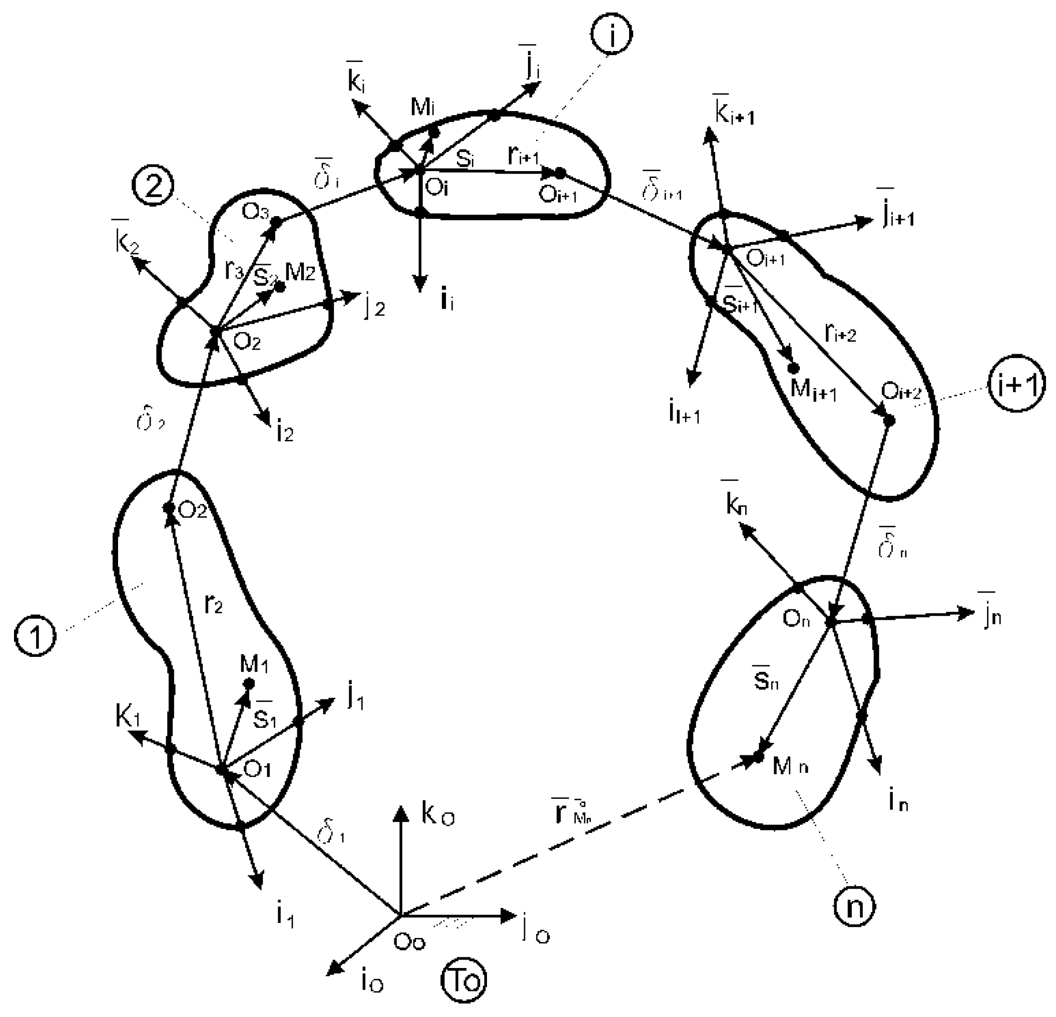
Figure 3.
Geometrical model of the elastic solid.
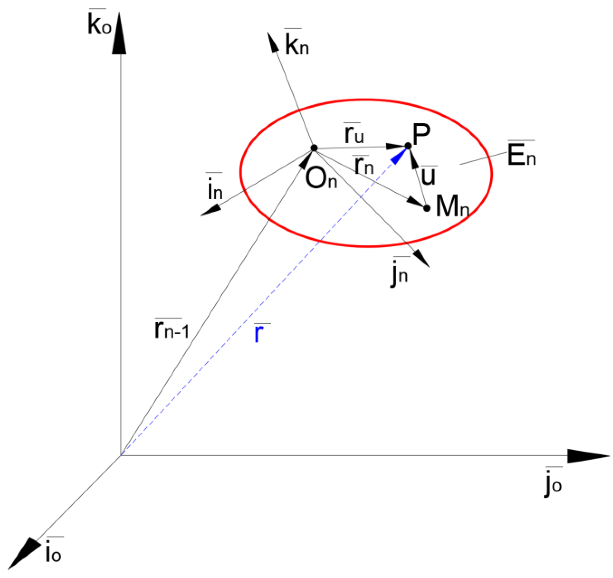
Figure 4.
Internal combustion engine mechanism components.
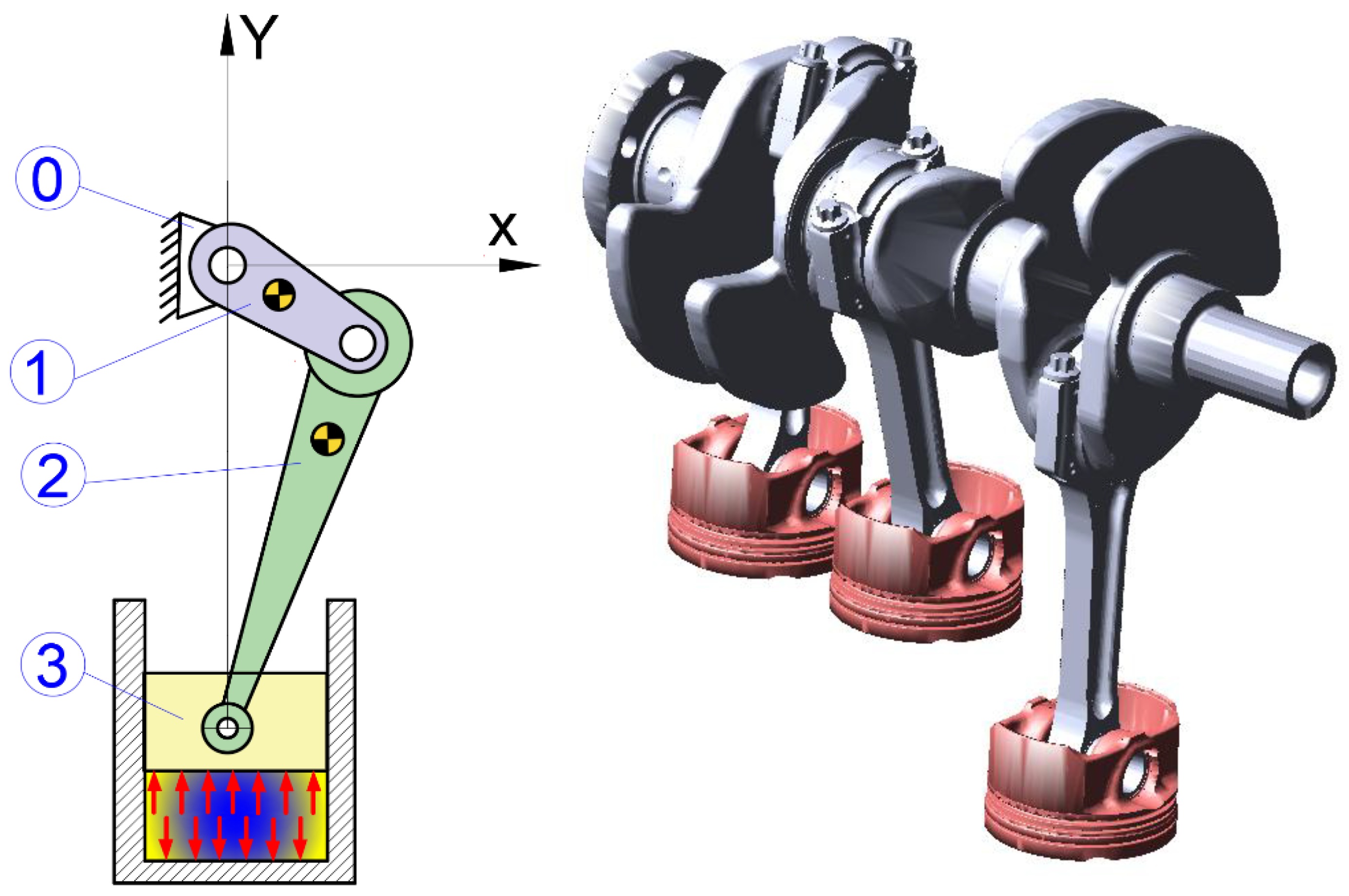
Figure 5.
Engine dynamic parameters variation depending on the crankshaft rotation angle.
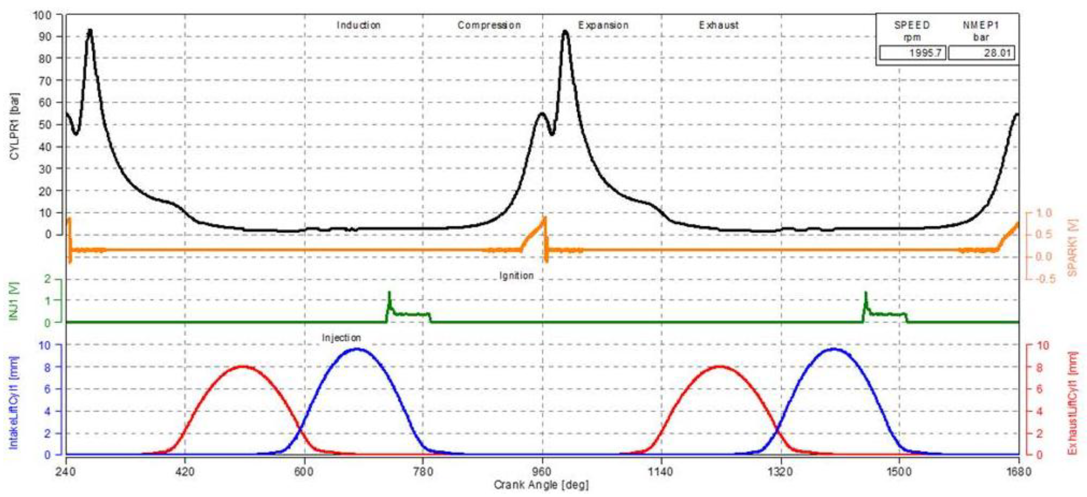
Figure 6.
Force variation developed by the gas on the piston head.
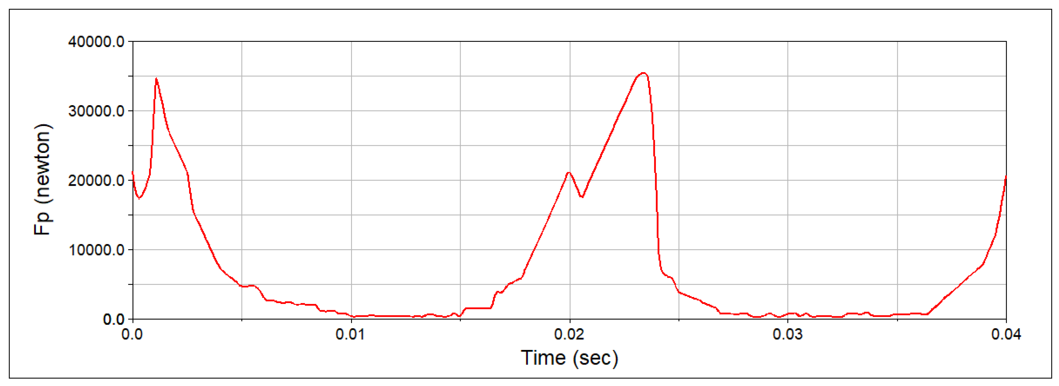
Figure 7.
Finite elements and nodes.
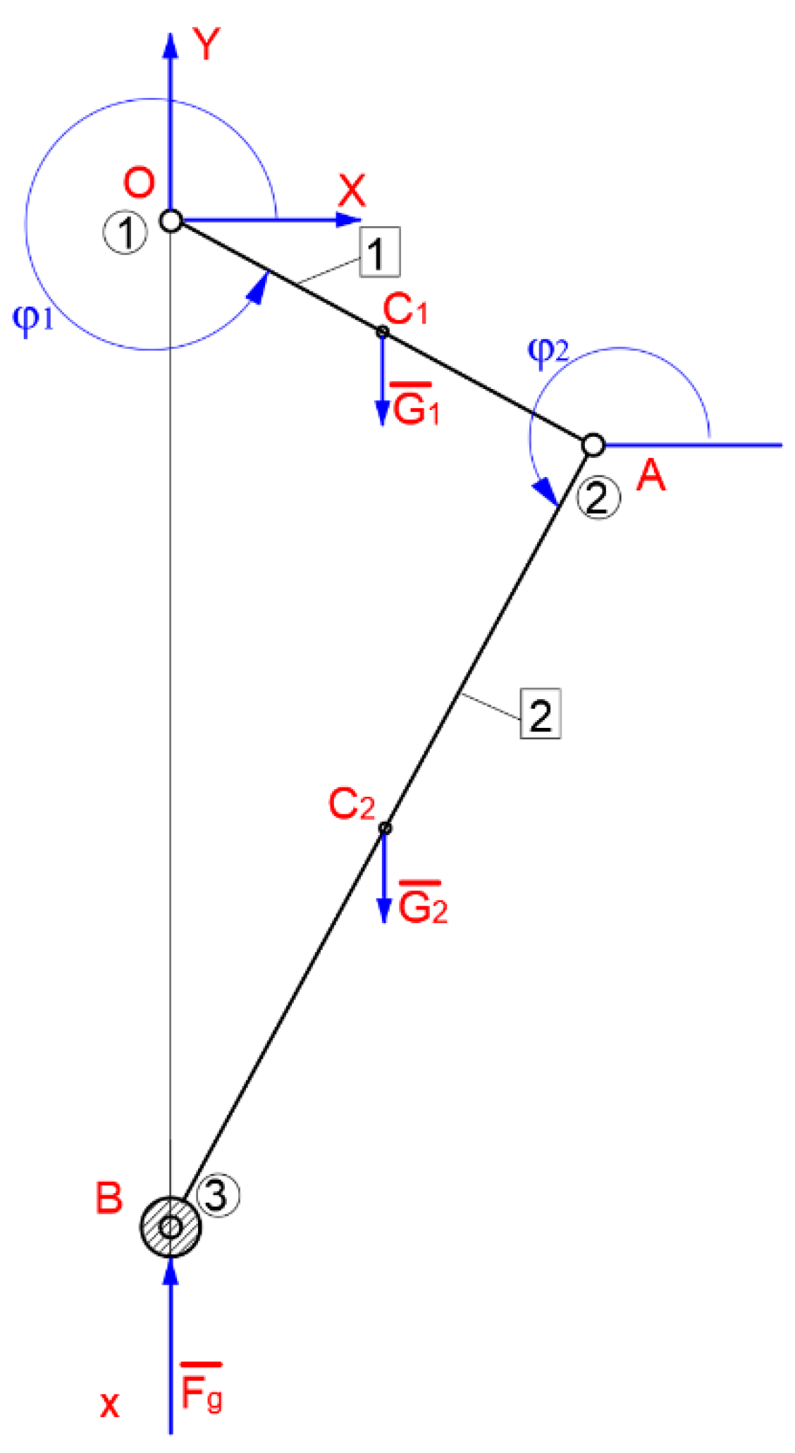
Figure 8.
Mechanism kinematic scheme.
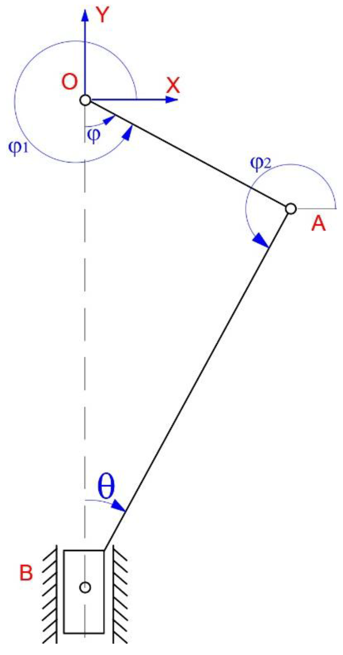
Figure 9.
Finite element no. 1.
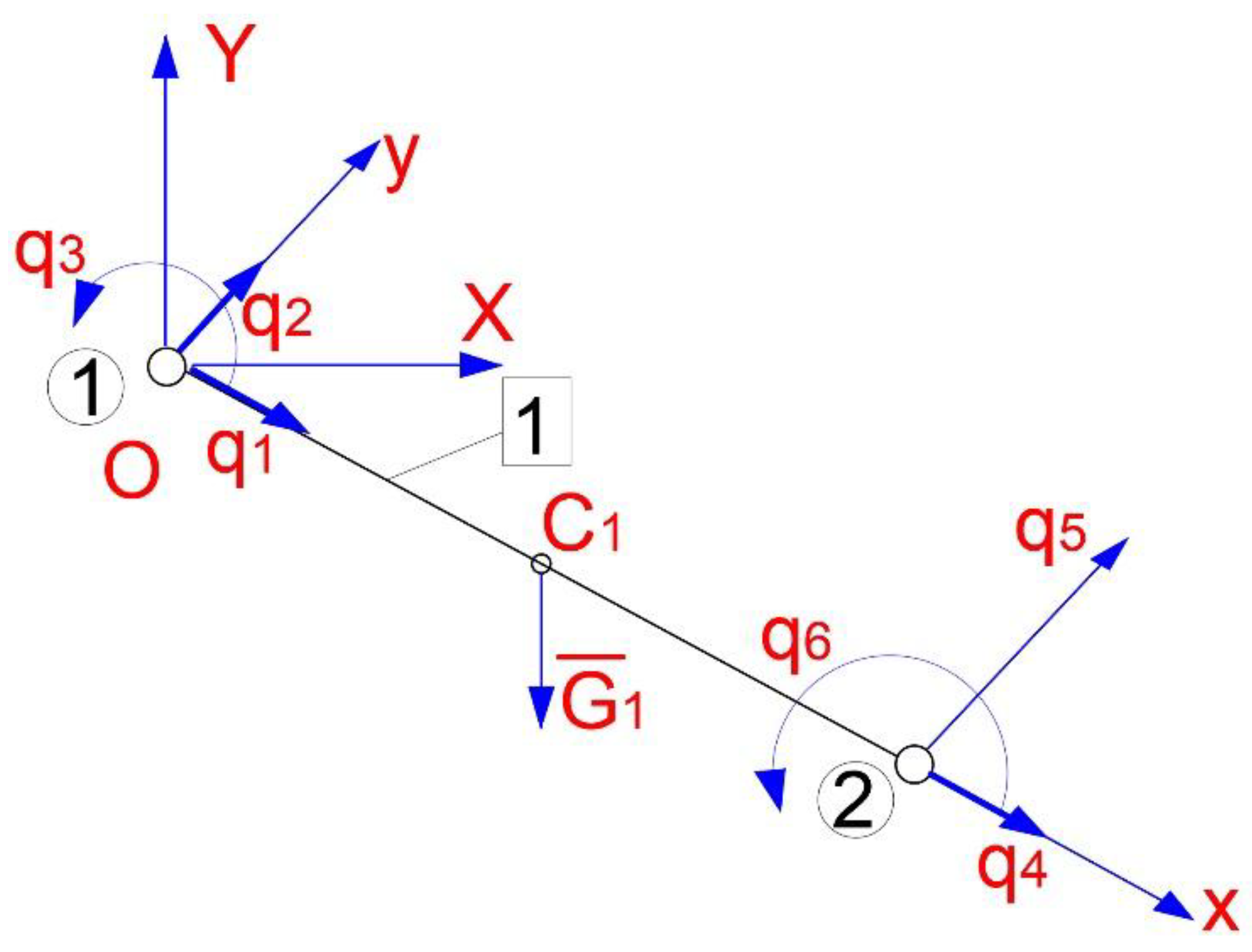
Figure 10.
Finite element no. 2.
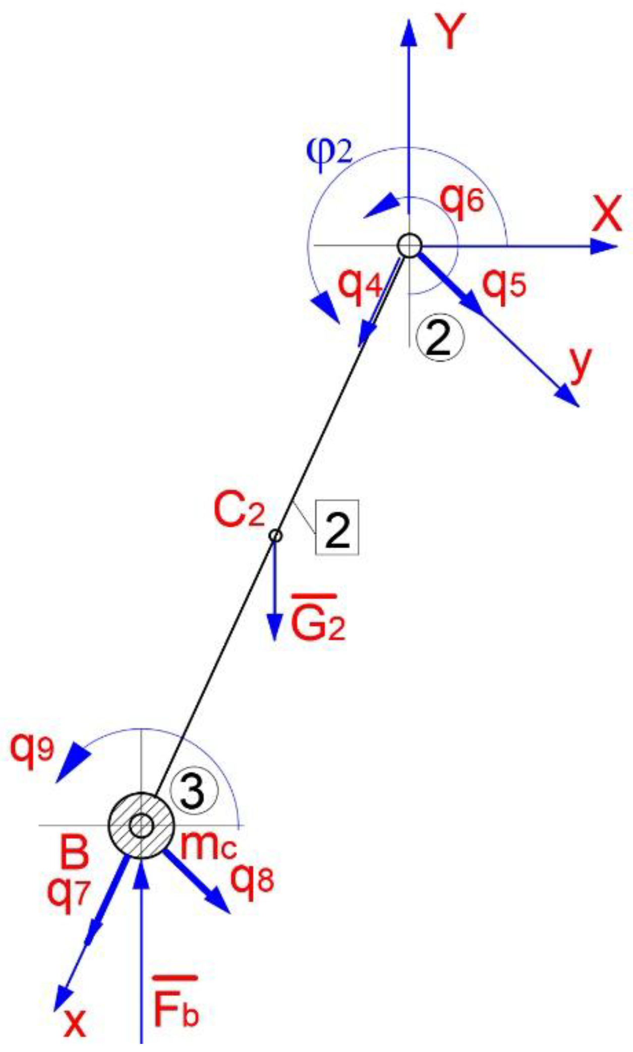
Figure 11.
Vibration mode no. 1, at f1 frequency.
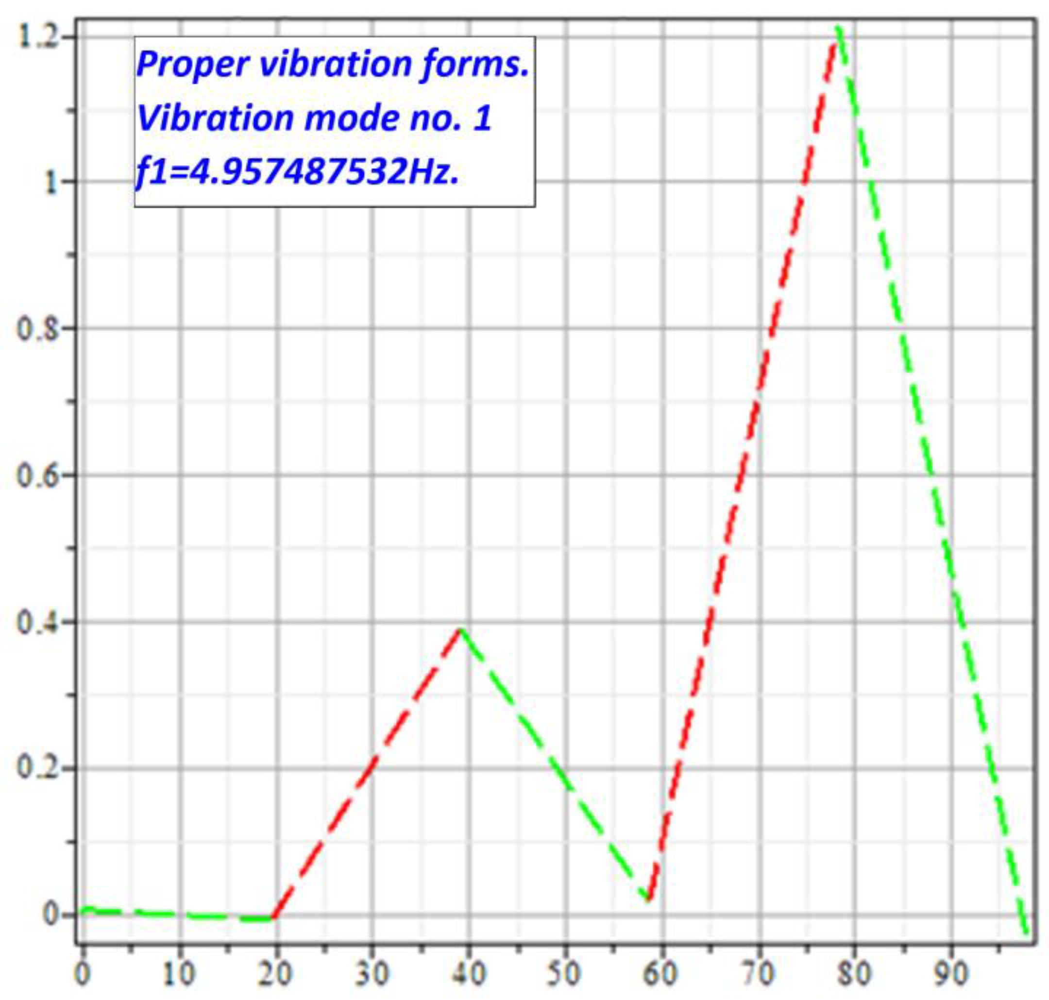
Figure 12.
Vibration mode no. 2, at f2 frequency.
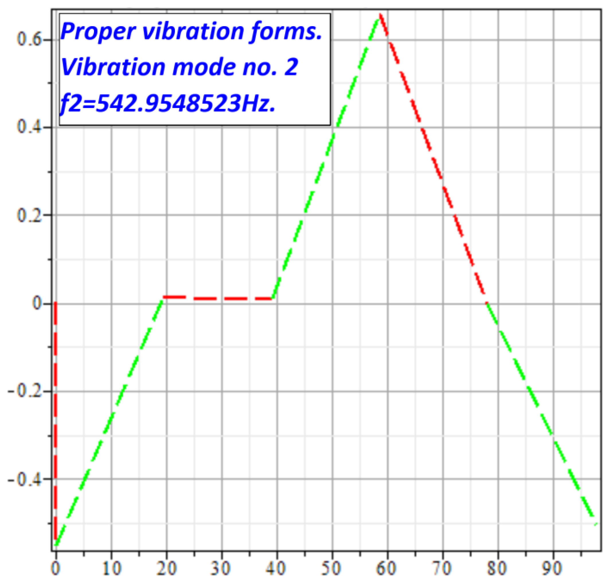
Figure 13.
Vibration mode no. 3, at f3 frequency.

Figure 14.
Vibration mode no. 4, at f4 frequency.

Figure 15.
Vibration mode no. 5, at f5 frequency.
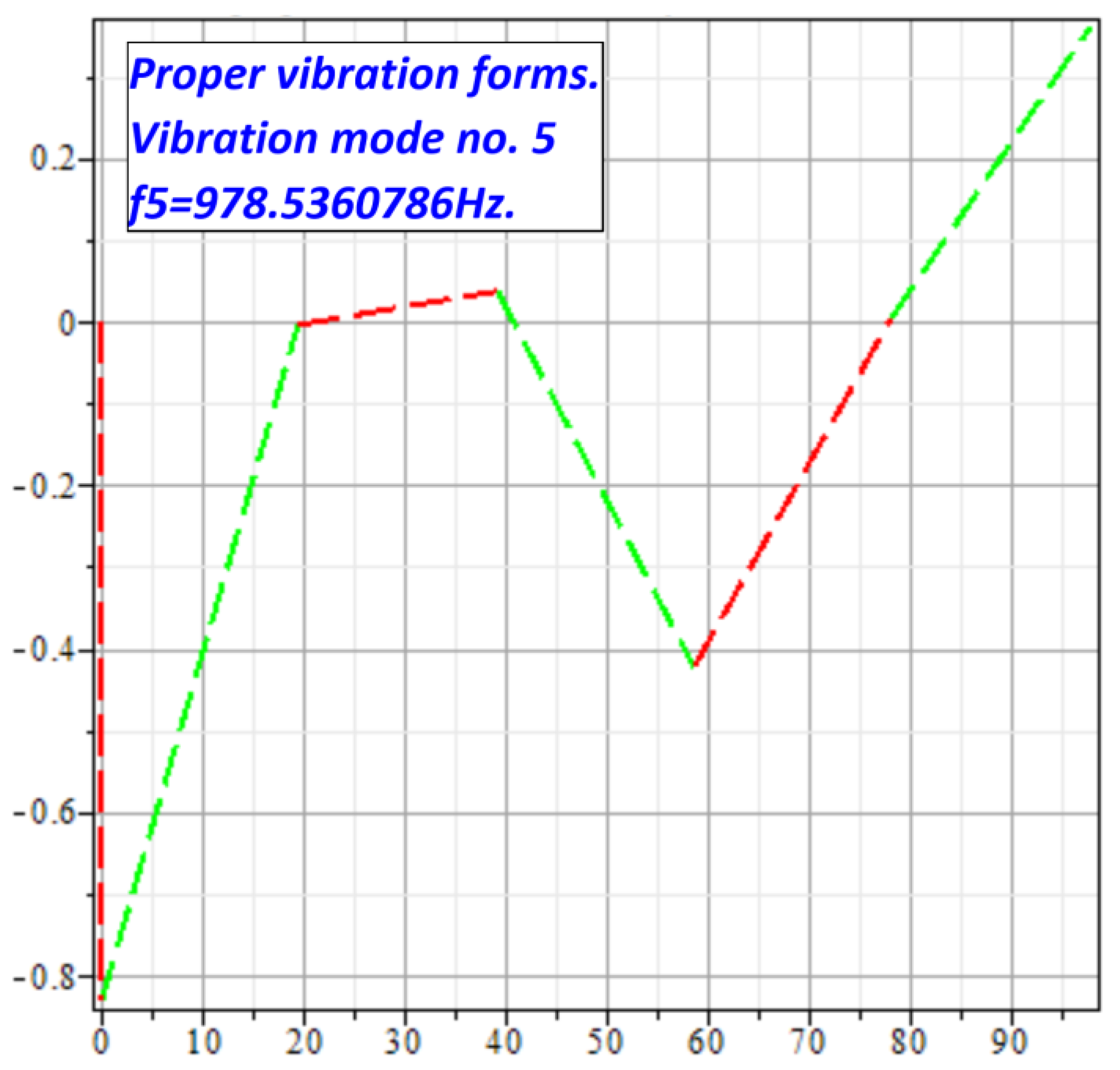
Figure 16.
Vibration mode no. 6, at f6 frequency.
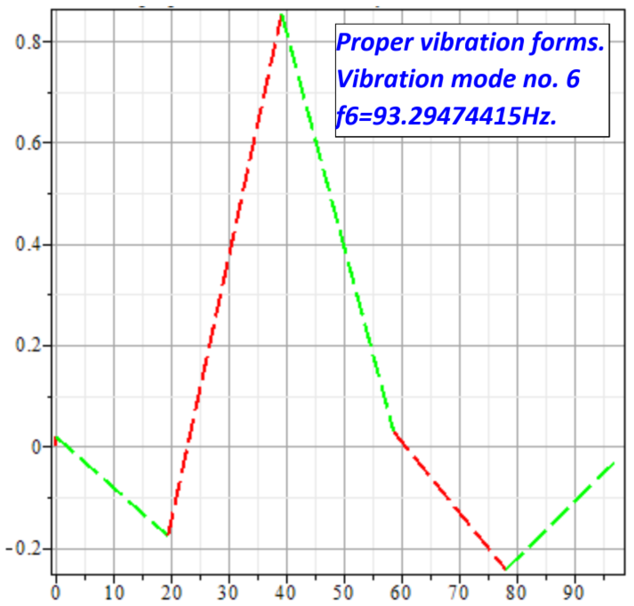
Figure 17.
Dynamic model from Adams (connecting rod 2 – mode 10, frequency 6425.318392722 Hertz).
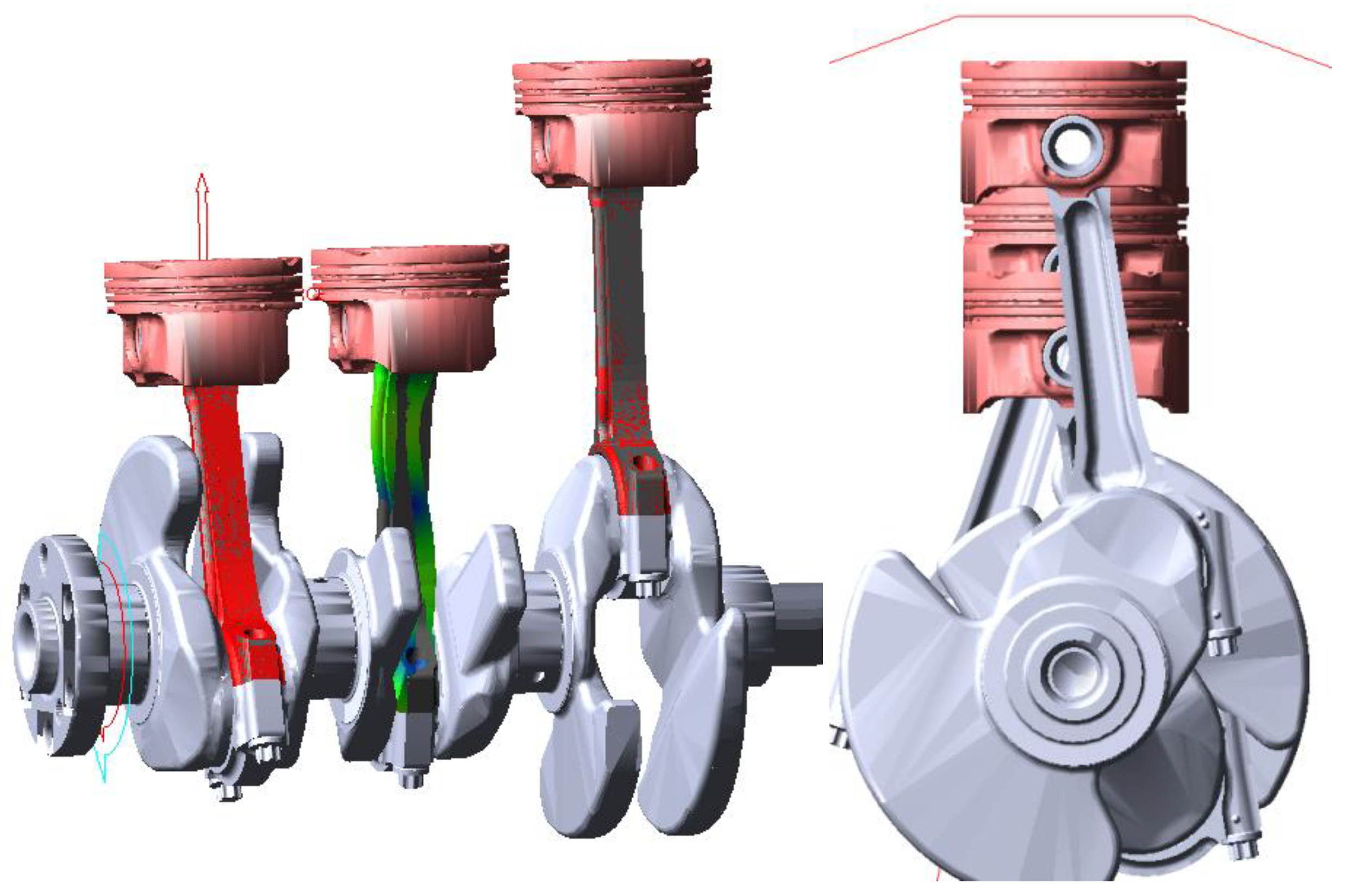
Figure 18.
Axial nodal displacement variation on x–axis (q4).
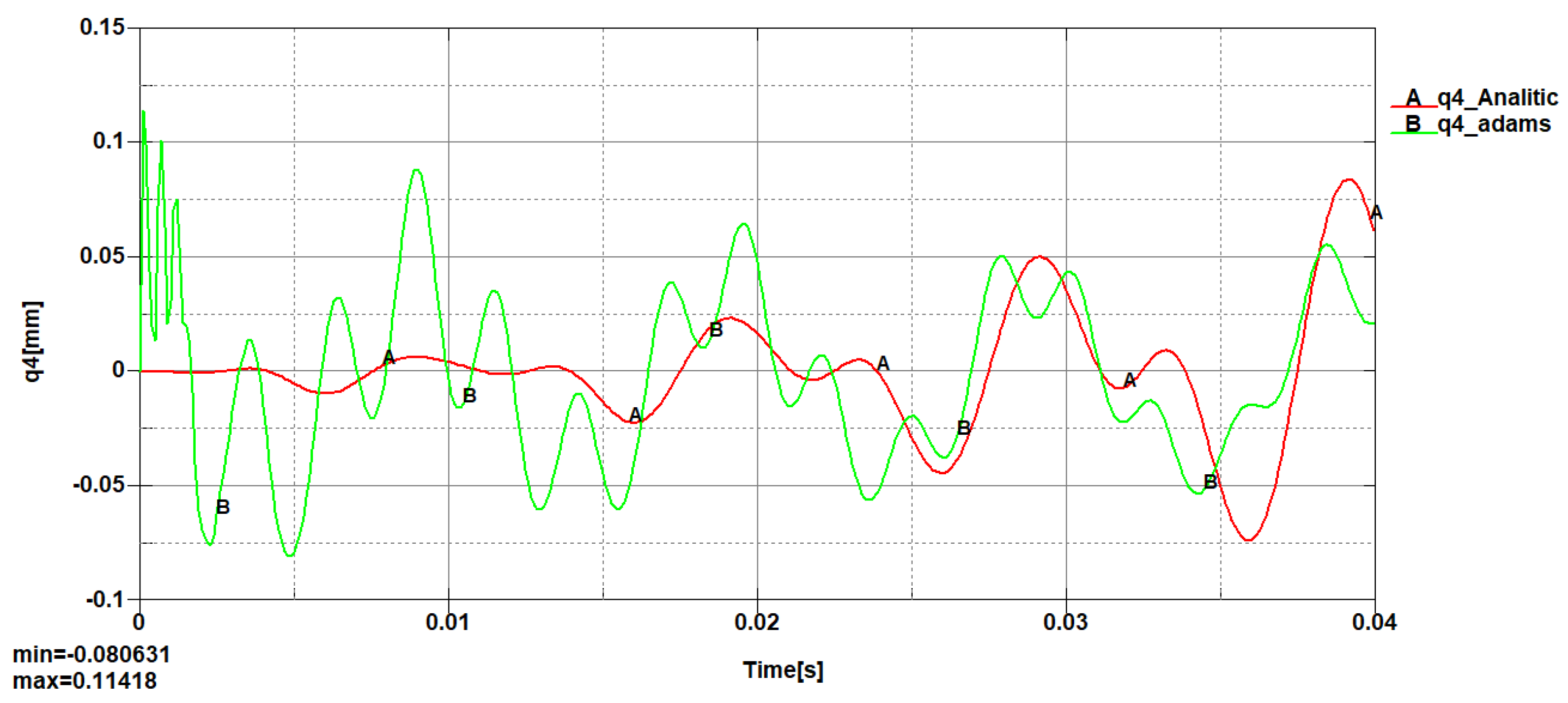
Figure 19.
Transversal nodal displacement variation on y–axis (q5).
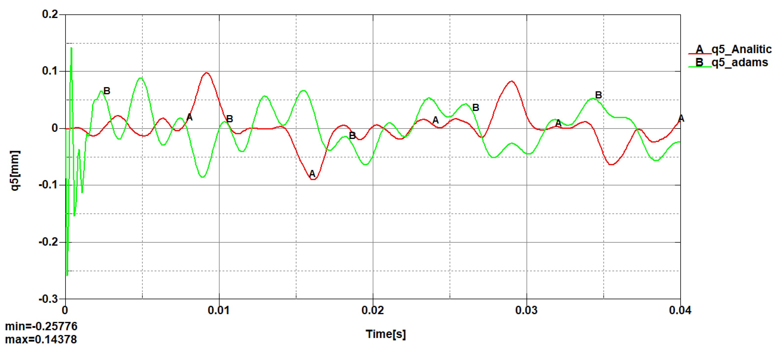
Figure 20.
Angular nodal displacement variation (q6).
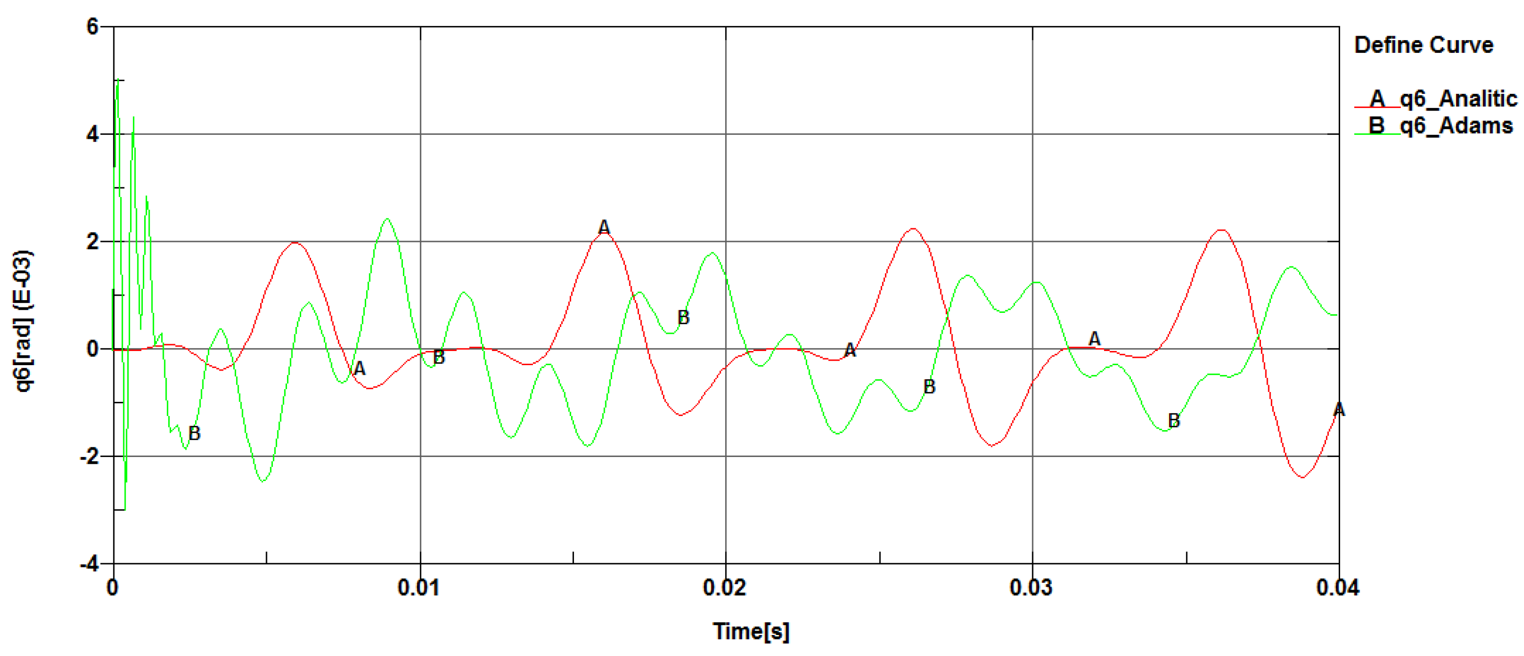
Figure 21.
Linear nodal displacement variation on x–axis (q7).
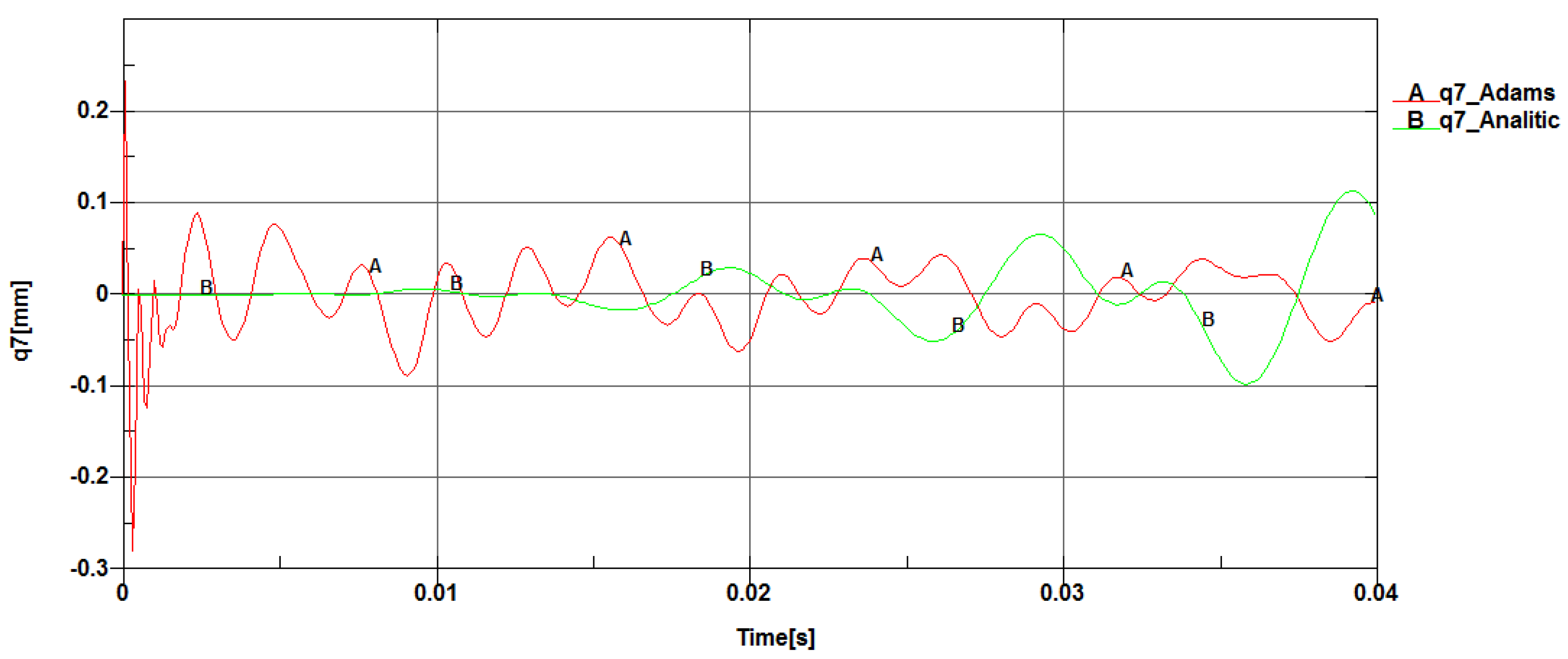
Figure 22.
Angular nodal displacement variation (q9).
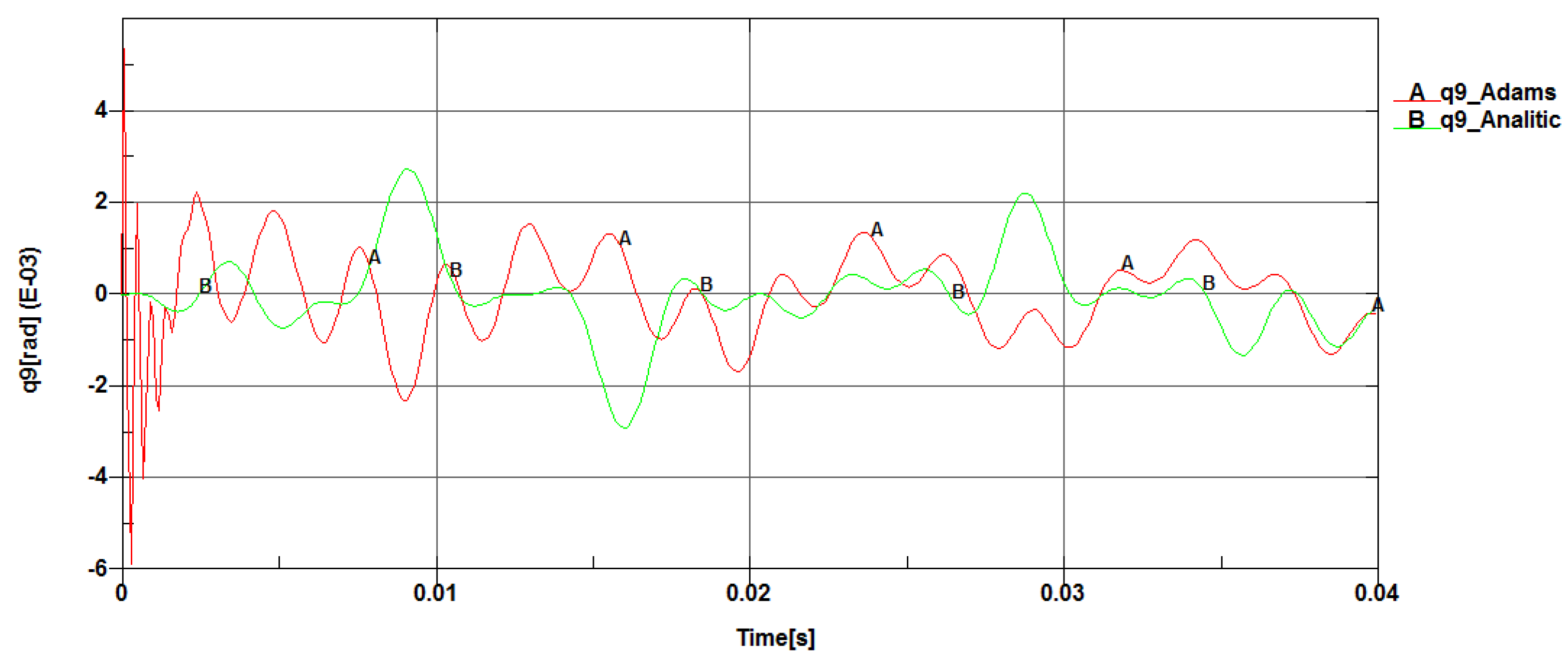
Figure 23.
Longitudinal elastic displacement, for the element no. 2 in the global coordinate system.
Figure 23.
Longitudinal elastic displacement, for the element no. 2 in the global coordinate system.
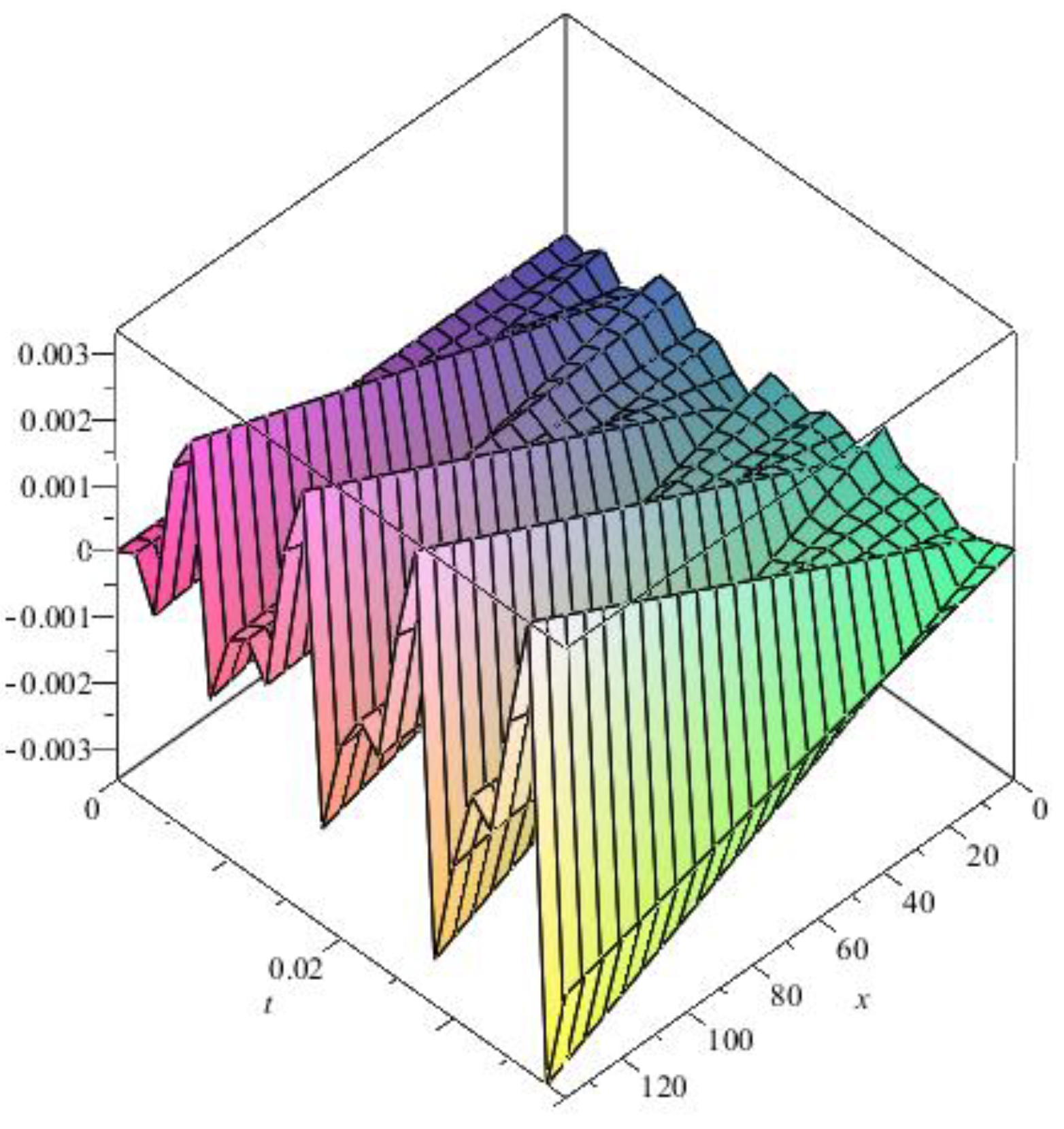
Figure 24.
Transversal elastic displacement, for element no. 2 in the global coordinate system.
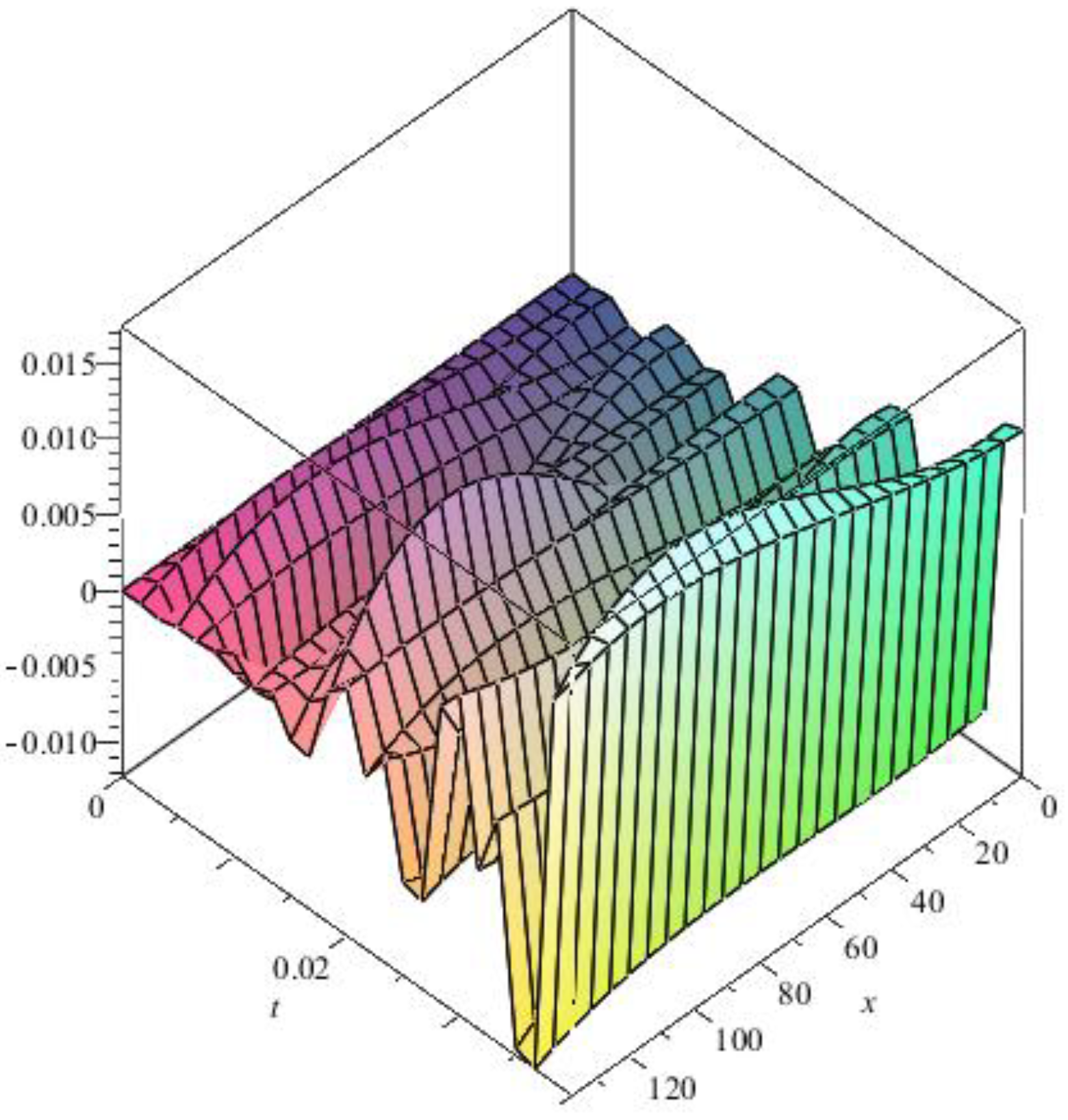
Figure 25.
Longitudinal displacement variation at half–length of the connecting rod length.
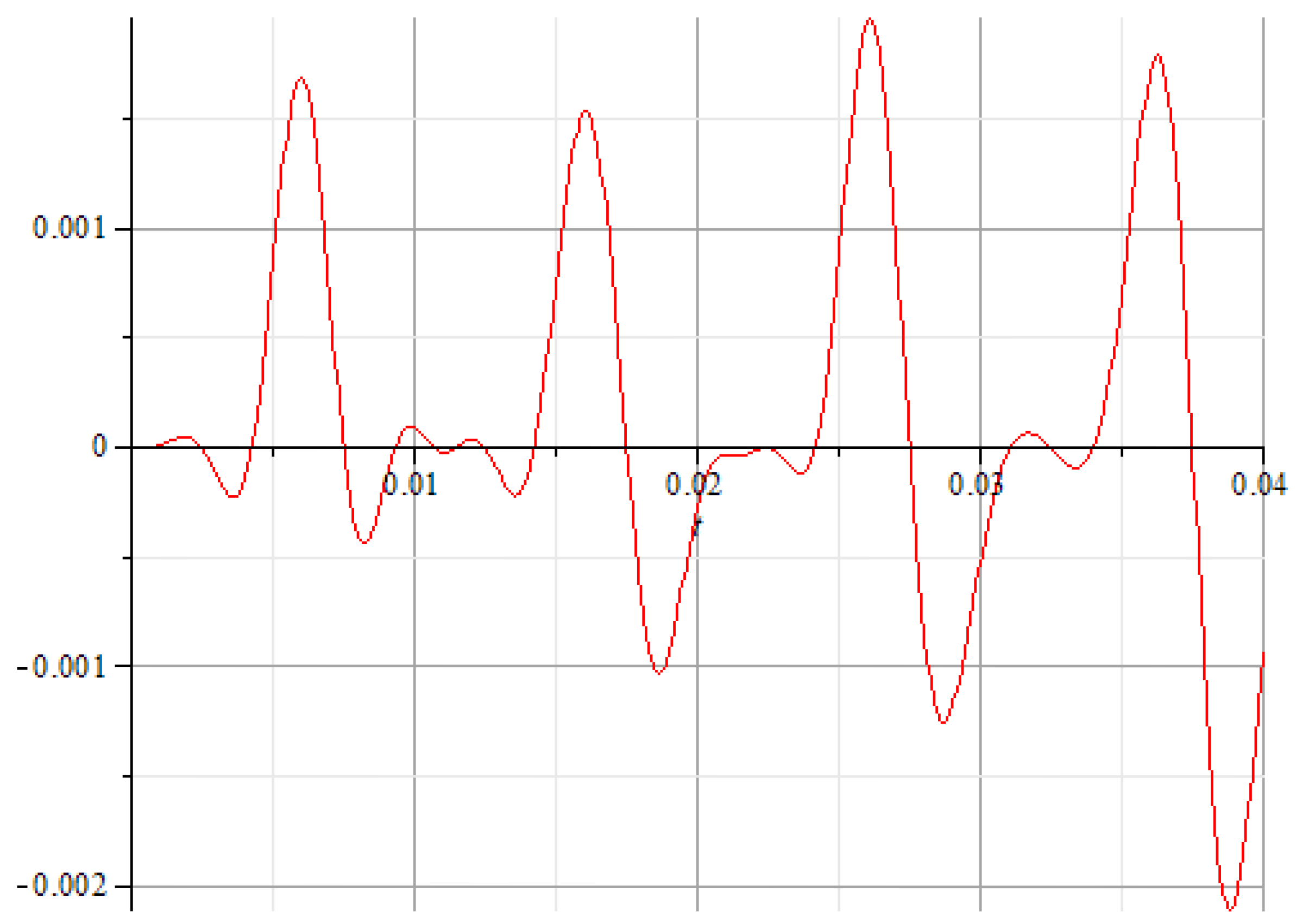
Figure 26.
Transversal displacements variation at half–length of the connecting rod length.
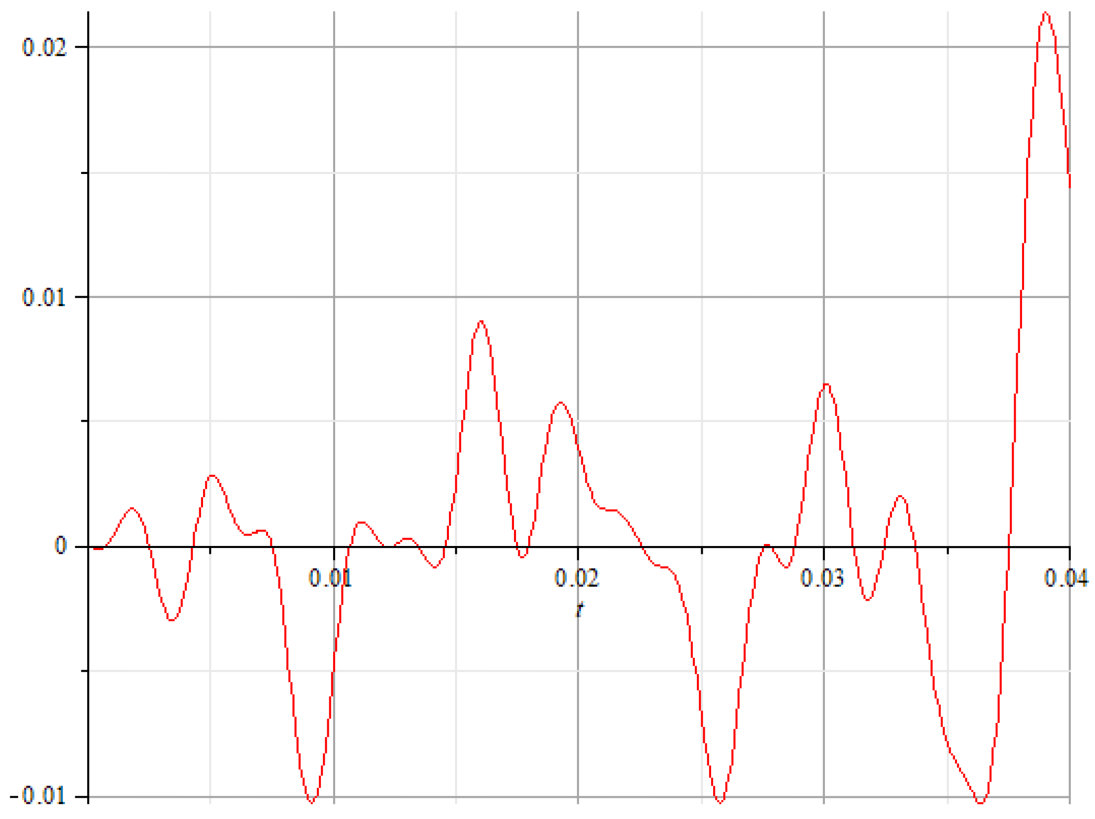
Figure 27.
Comparative analysis of the longitudinal elastic displacements.
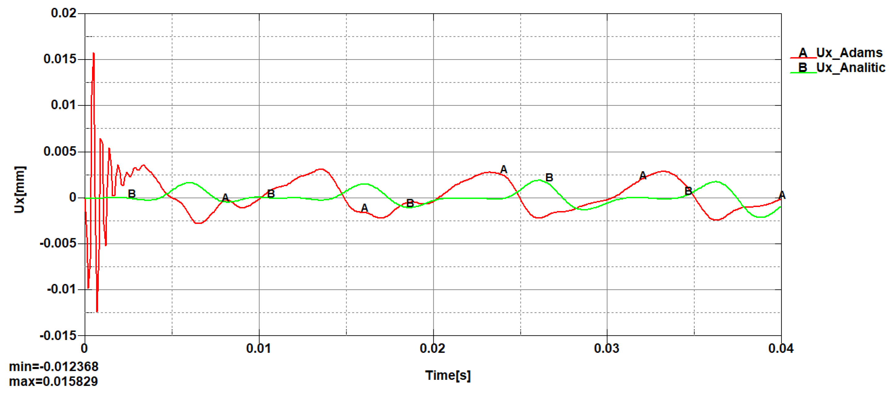
Figure 28.
Comparative analysis of the transversal elastic displacements.
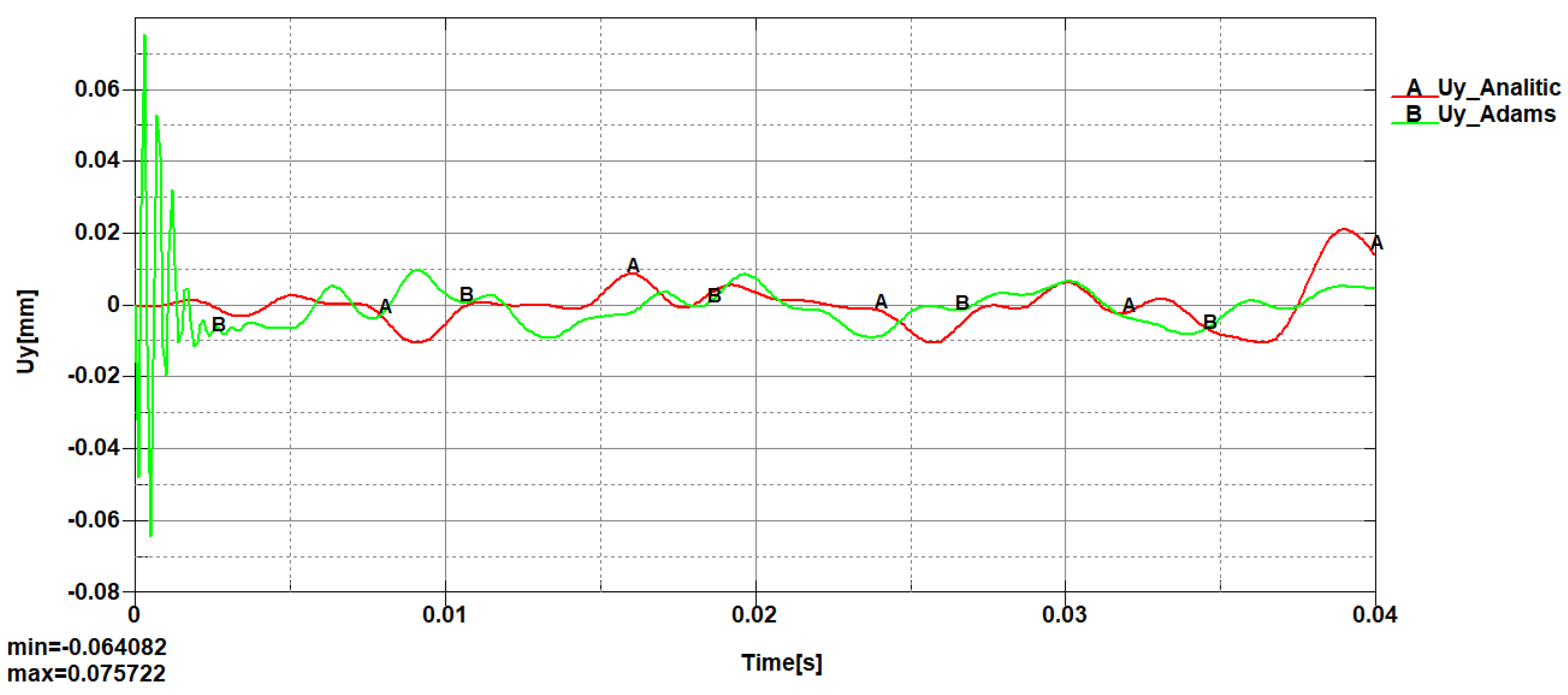
Figure 30.
Time analysis for recordings on the connecting rod at a frequency of 0.706 Hertz.
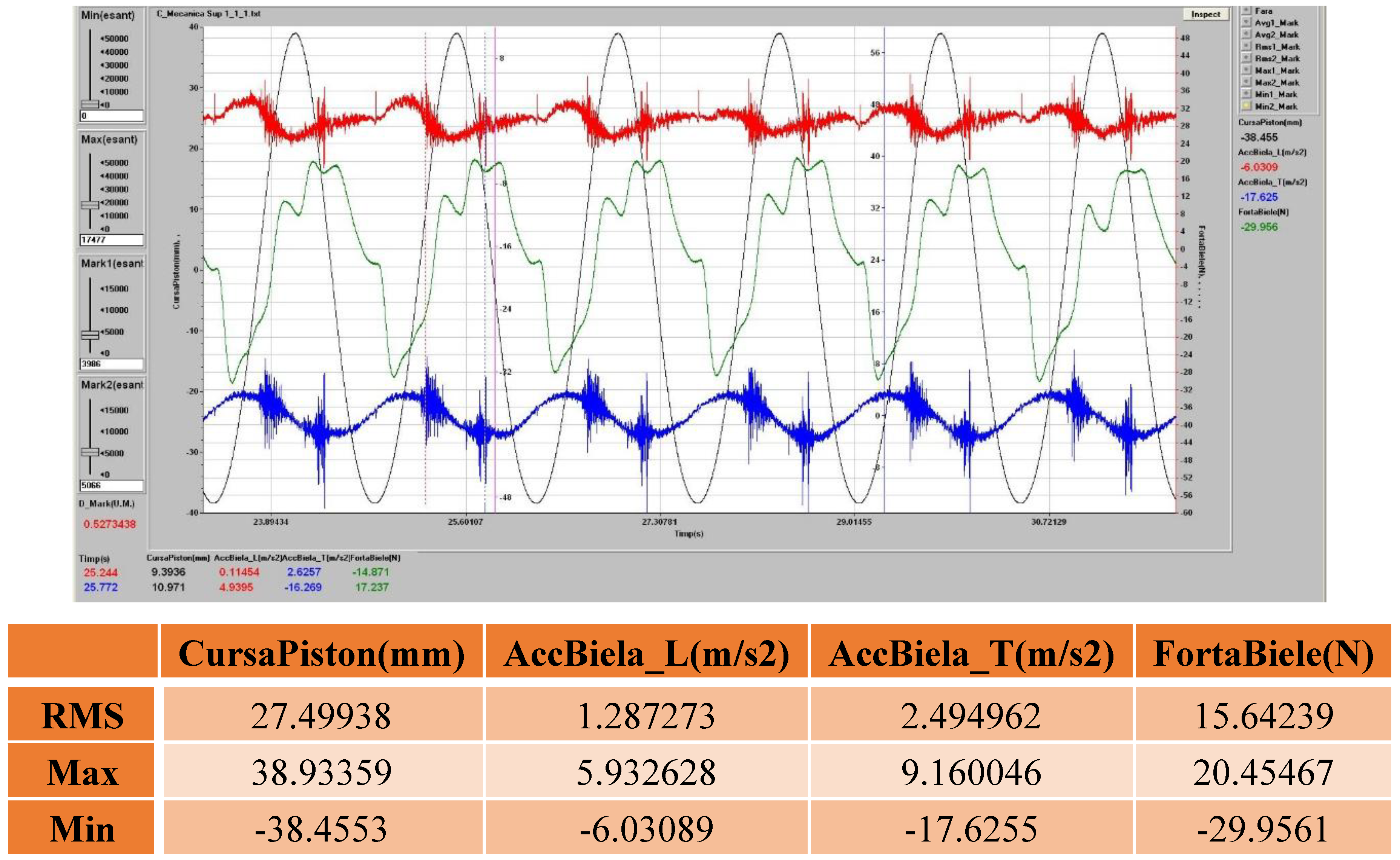
Figure 31.
Frequency analysis for recordings on the connecting rod at a frequency of 0.706Hertz.
Disclaimer/Publisher’s Note: The statements, opinions and data contained in all publications are solely those of the individual author(s) and contributor(s) and not of MDPI and/or the editor(s). MDPI and/or the editor(s) disclaim responsibility for any injury to people or property resulting from any ideas, methods, instructions or products referred to in the content. |
© 2025 by the authors. Licensee MDPI, Basel, Switzerland. This article is an open access article distributed under the terms and conditions of the Creative Commons Attribution (CC BY) license (http://creativecommons.org/licenses/by/4.0/).
Copyright: This open access article is published under a Creative Commons CC BY 4.0 license, which permit the free download, distribution, and reuse, provided that the author and preprint are cited in any reuse.


