Submitted:
07 July 2025
Posted:
08 July 2025
You are already at the latest version
Abstract
CO₂-WAG (Water-Alternating-Gas) injection is a vital technology for mitigating viscous fingering and gas channeling in CO₂ flooding processes, with the rational design of injection parameters being essential for low-permeability reservoirs. However, the significant heterogeneity and complex geological characteristics of these reservoirs introduce challenges in optimizing development parameters and accurately predicting production performance. This study developed 1,225 multivariate numerical simulation cases for CO₂-WAG and utilized XGBoost as the foundational machine learning framework. To optimize the model, four metaheuristic algorithms—Crowned Porcupine Optimization (CPO), Grey Wolf Optimizer (GWO), Artificial Hummingbird Algorithm (AHA), and Black Kite Algorithm (BKA)—were applied. Among these, CPO demonstrated superior performance in handling high-dimensional, complex problems due to its balanced global search and local exploitation capabilities. Further improvements were achieved by integrating Chebyshev chaotic mapping and an elite opposition-based learning (EOBL) strategy, leading to the development of the ICPO (Improved Crowned Porcupine Optimization)-XGBoost model. The ICPO-XGBoost model achieved exceptional predictive performance, with a coefficient of determination R² of 0.9894 and a root mean square error (RMSE) of 2.894, while maintaining prediction errors within 2%. These results validate the model’s stability, reliability, and generalization capabilities, offering a robust and innovative solution for CO₂-WAG parameter optimization in low-permeability reservoirs.
Keywords:
low-permeability reservoirs
; CO2 water-alternating-gas injection
; machine learning
; extreme gradient boosting
; crowned porcupine optimization (CPO)
1. Introduction
Low-permeability reservoirs, as a crucial component of unconventional oil and gas resources, pose significant technical challenges for enhanced oil recovery (EOR) in the petroleum industry [1]. Characterized by low permeability and porosity, these reservoirs limit the effectiveness of traditional development techniques [2]. Recently, CO2 Water-Alternating-Gas (CO2-WAG) injection has emerged as a promising EOR technology for low-permeability reservoirs due to its dual benefits of improving oil recovery and facilitating CO2 geological sequestration [3,4,5,6]. By synergizing gas injection and water flooding mechanisms, CO2-WAG enhances displacement efficiency, expands the sweep volume, and mitigates gas channeling [7]. However, the strong heterogeneity and complex pore-throat structures of low-permeability formations constrain CO2 and water migration, introducing uncertainties in fluid sweep efficiency and production performance [8,9]. Consequently, optimizing development parameters and accurately predicting production performance during CO2-WAG implementation remain critical challenges.
Traditional reservoir prediction methods, including empirical formulas, reservoir engineering analyses, and numerical simulations, have been widely employed [10].While empirical and reservoir engineering methods are effective under specific geological and operational conditions, their applicability is often limited to narrow scenarios [11,12]. Numerical simulation methods provide a detailed representation of multiphase fluid flow in porous media and are considered the cornerstone of conventional reservoir prediction [13]. However, as reservoir heterogeneity increases and multi-parameter conditions are introduced, the computational burden of numerical simulations grows exponentially. Single simulation cases may require hours or even days to complete, making them impractical for real-time reservoir management [14,15]. Thus, achieving rapid optimization of development parameters while maintaining high prediction accuracy remains a pressing research need.
Advances in artificial intelligence (AI) and data science have recently shown the potential of machine learning (ML) in petroleum engineering[16]. ML models excel at handling complex nonlinear systems, accelerating history matching, and avoiding the convergence issues associated with traditional methods [17,18,19,20]. Leveraging high-quality numerical simulation data, ML models can efficiently learn the underlying dynamics of reservoir systems, enabling rapid production forecasting and development optimization [21]. For instance, You et al. developed an ML-based optimization workflow integrating artificial neural networks (ANN) with particle swarm optimization (PSO) to enhance oil recovery and CO2 sequestration efficiency in CO2-WAG projects [22]. Similarly, Vo Thanh et al. evaluated four ML models (GRNN, CFNN-LM, CFNN-BR, and XGBoost) for predicting oil recovery factors (ORF) in CO2 foam flooding, demonstrating significant reductions in experimental costs and time [23]. Other studies have combined ML algorithms with optimization techniques to achieve substantial improvements in CO2-WAG parameter optimization and production forecasting [24,25].
Despite these advancements, ML algorithms face challenges such as sensitivity to initial values, complex hyperparameter tuning, difficulty in handling high-dimensional data, and limited multi-objective optimization capabilities. As a solution, metaheuristic algorithms have gained prominence as powerful tools for nonlinear, non-convex, and multi-objective optimization problems [26]. Unlike traditional optimization methods, metaheuristic algorithms efficiently explore solution spaces under constrained computational resources, providing satisfactory approximations for complex engineering scenarios. For example, Menad et al. combined a multilayer perceptron (MLP) neural network with the Non-Dominated Sorting Genetic Algorithm II (NSGA-II) to optimize CO2-WAG injection parameters under multi-objective constraints [27]. Gao et al. integrated XGBoost with PSO to develop a proxy model for optimizing CO2-EOR parameters [28], while Kanaani et al. employed stacking learning and NSGA-II to optimize oil production, CO2 storage, and net present value (NPV) in CO2-WAG projects [29].
While the integration of metaheuristic algorithms and ML technologies has shown great potential, effectively combining multivariable numerical models, data-driven methods, and physical displacement mechanisms remains a significant challenge. This study introduces an ICPO (Improved Crowned Porcupine Optimization)-XGBoost model specifically designed for CO2-WAG development in low-permeability reservoirs. The XGBoost algorithm serves as the core ML framework, while four metaheuristic algorithms inspired by natural behaviors—Crowned Porcupine Optimization (CPO), Artificial Hummingbird Algorithm (AHA), Black Kite Algorithm (BKA), and Grey Wolf Optimizer (GWO)—are employed to optimize hyperparameters. Six critical parameters are considered—bottom-hole pressure, water-gas ratio, gas injection rate, water injection rate, oil production rate, and injection duration—to predict cumulative oil production under CO2-WAG conditions. To further enhance CPO’s efficiency and adaptability to complex reservoir conditions, Chebyshev chaotic mapping and Elite Opposition-Based Learning (EOBL) strategies are incorporated, improving its convergence efficiency and robustness. By integrating data-driven approaches with physical displacement mechanisms, this study bridges the gap between traditional empirical methods and modern ML models, achieving enhanced prediction accuracy and physical consistency. The proposed framework offers robust support for real-time production optimization and early warning systems in field operations.
The remainder of this paper is organized as follows: Chapter 2 outlines the reservoir model construction and dataset generation process. Chapter 3 introduces the ICPO-XGBoost model and compares its performance with other newly proposed algorithms. Chapter 4 evaluates the predictive performance of various optimization models, analyzes the importance of decision variables, and validates the proposed model’s accuracy and stability. Finally, Chapter 5 summarizes the key findings and practical implications of this study.
2. Model Description and Dataset Construction
2.1. Reservoir Model
This study examines a block from a typical low-permeability oil reservoir in China to evaluate the application of CO2-WAG flooding technology in complex heterogeneous reservoirs. The primary structural feature of the study area is an anticlinal nose, with sandstone as the dominant reservoir type. The lithology primarily comprises fine sandstone and siltstone, interspersed with localized mudstone and carbonate rock intercalations (Figure 1). The reservoir has an average burial depth of 3,150 m, and the study area spans 778 × 1,427 × 218 m, encompassing a total grid count of 46,056. This grid configuration effectively captures the spatial complexity and heterogeneity of the reservoir.
The principal reservoir properties include an initial pressure of 43.9 MPa, porosity ranging from 1.2% to 8.9% (average 6.4%), and permeability between 0.015 mD and 30 mD (average 1.05 mD), classifying it as a typical low-permeability reservoir. The crude oil is characterized by a high content of light components and a low fraction of heavy components, indicating favorable fluidity and significant potential for enhanced oil recovery.
Based on laboratory PVT data, a nine-component fluid model was developed (Table 1), providing a robust foundation for numerical simulations. Figure 2 illustrates the relative permeability curves for oil-water and oil-gas systems, derived from laboratory core analyses under varying water and gas saturation conditions. To explore the influence of injection and production parameters on development performance, a five-spot well pattern was implemented, comprising nine vertical wells: four injection wells (Inj1 to Inj4) and five production wells (Prod1 to Prod5), with an average well spacing of 280 m. CO2-WAG technology was employed to alternate gas and water injection, enhancing oil recovery. Production performance was simulated over a 20-year period, with results recorded at 1-year intervals.
2.2. Decision Variable Selection and Dataset Generation
Six parameters were selected as decision variables to evaluate the CO2-WAG development process: bottom-hole pressure of production wells (BHPO), water-to-gas ratio (WGR), gas injection rate (RATEG), water injection rate (RATEW), oil production rate (ORAT), and injection cycle (IC). The cumulative oil production (OPRO) was defined as the objective function to assess the impact of these parameters on development performance. The ranges of decision variables were determined based on geological constraints, engineering feasibility, and economic rationality. Table 2 summarizes the statistical properties of the decision variables, which were selected following these criteria:
- Geological Constraints: Variable ranges were defined to comply with reservoir properties. For instance, BHPO was constrained to remain above the bubble point pressure to prevent premature gas breakout and below the reservoir fracture pressure to ensure structural integrity. Similarly, RATEG and RATEW were restricted within the reservoir’s injection capacity to avoid fracturing.
- Engineering Feasibility: Values were chosen to align with practical field operation limits, ensuring system stability. For example, the WGR was constrained by the capacity of surface facilities and well designs, while the IC was optimized to prevent incomplete displacement and uneven fluid distribution.
- Economic Rationality: Parameter ranges were optimized to balance operational costs and economic returns. RATEG and RATEW were adjusted to maximize recovery efficiency while minimizing costs, and IC was optimized to enhance overall production efficiency.
To ensure a representative and evenly distributed dataset, the Latin Hypercube Sampling (LHS) method was employed. This approach ensured comprehensive coverage of the high-dimensional parameter space, avoiding clustering and blank regions typical of random sampling. A total of 1,225 samples were generated, with their characteristics summarized in Table 2. Figure 3(a) illustrates the Pearson correlation heatmap, highlighting the linear relationships between variables. OPRO exhibits a moderate positive correlation with RATEG (correlation coefficient = 0.34) and a significant negative correlation with WGR (correlation coefficient = -0.64), indicating their substantial influence on production performance. Other variables, such as BHPO and IC, show weaker correlations with OPRO, suggesting limited direct impacts. Figure 3(b) presents box plots of normalized variables, emphasizing their distributions and range variations. Normalization was conducted using the min-max scaling method to eliminate dimensional differences and improve data comparability.
2.2. Model Evaluation Metrics
To assess the predictive performance of the model, four evaluation metrics were employed: coefficient of determination (R2), root mean square error (RMSE), mean absolute error (MAE), and variance accounted for (VAF). The definitions of these metrics are as follows:
where, n is the number of samples; P is the observed values; is the mean of the observed values, and the predicted value. R2 quantifies the proportion of variance in observed data explained by the model, with values closer to 1 indicating better fit; RMSE measures the square root of the mean squared errors, with smaller values indicating higher accuracy; MAE represents the average absolute difference between observed and predicted values, offering robustness against outliers; VAF denotes the percentage of variance explained by the model, with values closer to 100% indicating better reliability.
3. Methodology
To address the complexity and significant nonlinear characteristics of parameter optimization in low-permeability reservoirs during CO2-WAG development, this study generated 1,225 datasets through numerical simulations, creating a multivariable dataset with OPRO defined as the objective function. Using this dataset, the feasibility of predicting complex reservoir development processes was explored through the application of the XGBoost model. To further enhance predictive performance, metaheuristic optimization algorithms were employed to tune the hyperparameters of XGBoost. Additionally, the CPO algorithm was enhanced through the integration of Chebyshev chaotic mapping and an EOBL strategy, resulting in the development of the ICPO-XGBoost model, which is tailored for CO2-WAG development in low-permeability reservoirs.
3.1. XGBoost
Traditional numerical simulation methods and empirical formulas often suffer from significant limitations, including high computational costs and insufficient prediction accuracy in addressing complex reservoir problems. In contrast, machine learning methods, particularly the XGBoost algorithm, offer distinct advantages in CO2-WAG development due to their robust nonlinear modeling capabilities and computational efficiency. XGBoost, a highly efficient and scalable machine learning algorithm based on gradient boosting tree models, has demonstrated strong predictive performance for both nonlinear problems and large-scale datasets. The core concept of XGBoost lies in iteratively constructing multiple weak learners (regression trees) to minimize residual errors, thereby enhancing overall prediction accuracy [30].
In the context of CO2-WAG development, parameters such as the RATEG, RATEW, WGR, and BHPO exhibit complex nonlinear interactions with reservoir dynamics. XGBoost captures these intricate dependencies by combining the outputs of multiple regression trees. During each iteration, XGBoost constructs a new regression tree based on the current model’s loss function, refining predictions by progressively minimizing residual errors [31]. The prediction output of XGBoost can be expressed as:
where, denotes the predicted value of the i-th sample; represents the prediction of the k-th tree for sample; F is the function space of tree models; defines the mapping from input feature space to leaf nodes; represents the prediction weight of each leaf node; T is the number of leaf nodes in the tree.
The optimization objective of XGBoost is to minimize the following objective function, which combines a loss term and a regularization term to balance prediction accuracy and model complexity:
where, is the objective function; represents the loss function, measuring the prediction error; is the regularization term, penalizing model complexity; denotes the set of model parameters; indicates the structure and leaf weights of a single tree.
The loss function quantifies the deviation between observed and predicted values:
The regularization term penalizes model complexity to enhance generalization capability:
where, is the penalty parameter for the number of leaf nodes; λ is the regularization parameter for leaf weights; By incorporating a regularization term, XGBoost mitigates the risk of overfitting and ensures stable performance on test data.
XGBoost optimizes the objective function through recursive iterations. During each iteration, a new regression tree is constructed to minimize the residual errors from the previous iteration. The algorithm leverages first-order and second-order derivative information of the loss function to enhance optimization efficiency, enabling accurate adjustments in predictions based on gradient information. Training terminates under one of the following conditions:
- The number of iterations reaches a predefined limit.
- The reduction in residuals falls below a specified threshold.
The model combines the outputs of multiple decision trees with corresponding weights, forming a highly accurate and computationally efficient regressor or classifier.
3.2. Hyperparameter Optimization Using Metaheuristic Algorithms
Hyperparameter optimization plays a critical role in enhancing the performance of machine learning models, particularly in high-dimensional and nonlinear problems such as CO2-WAG reservoir development. This study employs four up to date nature-inspired metaheuristic algorithms—Crowned Porcupine Optimization (CPO), Grey Wolf Optimization (GWO), Artificial Hummingbird Algorithm (AHA), and Black Kite Algorithm (BKA)—to optimize the hyperparameters of the XGBoost model. The integration of these algorithms ensures a robust balance between global exploration and local exploitation, improving the accuracy and generalization capability of the model.
3.2.1. Crowned Porcupine Optimization (CPO)
The Crowned Porcupine Optimization (CPO) algorithm is a recent metaheuristic method inspired by the defensive behaviors of crowned porcupines [32]. By simulating four distinct defensive strategies—visual, auditory, olfactory, and physical attacks—CPO dynamically balances global search and local refinement capabilities. This makes it highly effective for optimizing XGBoost hyperparameters in complex, high-dimensional parameter spaces [33]. Figure 4 illustrates the workflow of the CPO-XGBoost algorithm, and the optimization process can be summarized as follows:
- Data Preprocessing: The dataset is divided into training and testing subsets, and input features are normalized to eliminate dimensional biases and improve model stability.
- Population Initialization: Multiple candidate solutions, each representing a combination of hyperparameters, are randomly generated. Their fitness values are then evaluated to initialize the population.
-
Iterative Optimization: The CPO algorithm iteratively updates the population using a four-stage defensive strategy:
- First Defense Phase: Enhances solution diversity and broadens the search range by adjusting the distance between the predator and the target point, incorporating random perturbations.
- Second Defense Phase: Simulates auditory defense behavior to improve local search capability and diversify solutions.
- Third Defense Phase: Combines local perturbations with regional expansion to enhance global search capability.
- Fourth Defense Phase: Simulates elastic collisions, avoiding local optima and improving global search efficiency.
The specific computational methods for each phase are as follows:
- First Defense Phase: This phase enhances solution diversity and expands the search range by adjusting the distance between the predator and the target point, incorporating random factors. The update formula is:
- 2.
- Second Defense Phase: Simulating the porcupine’s auditory defense behavior, this phase enhances local search capability and further diversifies solutions. The update formula is:
- 3.
- Third Defense Phase: This phase improves global search capability by combining local perturbations with regional expansion. The update formula is:
- 4.
- Fourth Defense Phase: This phase simulates elastic collisions to improve global search ability and avoid local optima. The update formula is:where, denotes the best solution at iteration ; denotes the position of the -th individual at iteration ; and correspond to the positions of two randomly selected individuals; , ,…, are random values in [0, 1], controlling update magnitude; and are two random integers within [0, N], where N is population size; is randomly generated and contains elements that are either 0 or 1; The position of the predator is represented by , while serves as a parameter to control the search direction; defines the odor diffusion factor, and is the adjustment factor; indicates the resistance experienced by individual i during iteration t.
The CPO-XGBoost algorithm effectively improves model accuracy and generalization by optimizing hyperparameters through these defensive strategies.
3.2.2. Grey Wolf optimization (GWO)
The Grey Wolf Optimization (GWO) algorithm is a nature-inspired technique based on the hierarchical hunting behaviors of grey wolves [34]. The algorithm simulates the leadership hierarchy—alpha (α), beta (β), delta (δ), and subordinate wolves—and their cooperative hunting strategies to achieve global optimization. Each wolf adopts a search strategy according to its role, effectively avoiding local optima.
Figure 5 presents the workflow of the GWO-XGBoost algorithm. Initially, the positions of grey wolves are randomly generated, each position corresponding to a set of XGBoost hyperparameters. The fitness value of each wolf is evaluated based on the XGBoost model’s performance on the training dataset. The top three wolves are designated as alpha (α), beta (β), and delta (δ), representing the best, second-best, and third-best solutions, respectively. The remaining wolves follow their guidance to explore the global optimum. The position updates are defined as:
where, D represents the distance between the current position of the grey wolf and the target prey; denotes the position of the target prey; represents the current position of the grey wolf; , where a is the iteration parameter (decreasing with iterations) and is a random number; , with as a random number introducing perturbations.
3.2.3. Artificial Hummingbird Algorithm (AHA)
The Artificial Hummingbird Algorithm (AHA) is a novel swarm intelligence optimization technique inspired by the hovering flight and dynamic foraging behavior of hummingbirds [35]. By simulating the process of hummingbirds searching for and utilizing high-quality food sources, the algorithm effectively balances global exploration and local exploitation to solve complex optimization problems. AHA uses three flight modes—axial, diagonal, and omnidirectional flight—and three intelligent foraging strategies: guided foraging, local foraging, and migratory foraging [36]. These mechanisms collectively enhance the algorithm’s ability to explore the solution space and refine candidate solutions.
As shown in Figure 6, the AHA-XGBoost algorithm begins by calculating the fitness of each hummingbird (representing a hyperparameter combination). Based on the foraging strategy and flight mode, the positions of the hummingbirds are updated, and the fitness values are recalculated. The process continues until convergence is achieved, yielding the optimal hyperparameters for the XGBoost model.
where, represents the flying skill; i = rand [1, d] generates a random integer within the range [1, d], where d denotes the dimensionality of the search space; creates a random permutation of integers from 1 to ; represents a uniformly distributed random number between 0 and 1.
3.2.4. Black Kite Algorithm(BKA)
The Black-Winged Kite Algorithm (BKA) is an optimization technique inspired by the hunting and migration behaviors of black-winged kites [37]. By combining global search strategies with local exploitation, BKA effectively addresses complex optimization problems. In the framework of the BKA-XGBoost algorithm (Figure 7), BKA optimizes the hyperparameters of the XGBoost model by iteratively improving candidate solutions. Initially, the positions of the kite population are randomly initialized, with each position corresponding to a set of XGBoost hyperparameters. The user predefines the population size and search range.
During the attack phase, BKA simulates the behavior of kites approaching their target. The positions are updated using a dynamic scaling factor (n) and random perturbations (r), ensuring a smooth transition from global exploration to local exploitation. The update formula is:
where, represent the position of the i-th black-winged kite in the j-th dimension at the t-th iteration steps; r represents a random number between 0 and 1; g is a constant, often set to 0.9; T represents the total number of iterations, and denotes the number of iterations completed so far.
3.3. Enhanced Algorithm
The CPO-XGBoost algorithm has demonstrated exceptional performance in optimizing CO2-WAG development parameters for low-permeability reservoirs. Its strengths include high prediction accuracy, minimal error distribution, strong generalization ability, and excellent adaptability to complex nonlinear relationships. By effectively balancing global search and local exploitation, the algorithm mitigates overfitting and ensures consistent performance across both training and testing datasets. Additionally, it outperforms other comparative algorithms in terms of error metrics, showcasing superior stability and reliability. Detailed comparative results are presented in Chapter 4. However, the CPO-XGBoost algorithm has certain limitations. Its optimization process requires substantial computational resources, especially when applied to large-scale datasets, resulting in extended computation times. Furthermore, its performance is highly dependent on hyperparameter tuning, making it sensitive to configuration in complex engineering environments. This often necessitates meticulous debugging and adjustments.
To address the limitations of the original CPO algorithm, such as slow convergence speed, suboptimal optimization performance, and inefficient resource allocation, this study introduces two key improvements: the Chebyshev chaotic mapping mechanism and the EOBL strategy. These enhancements target the critical stages of population initialization and population updating [38]. The improved algorithm, termed ICPO, increases population diversity, enhances global search capabilities, and improves convergence efficiency, effectively overcoming the shortcomings of the original CPO algorithm.
3.3.1. Method Population Initialization via Chebyshev Chaotic Mapping
The original CPO algorithm utilizes a random initialization strategy to generate the initial population within the search space. While straightforward, this approach often results in high randomness and uneven distribution, leading to insufficient population diversity and suboptimal search performance. To address this issue, the Chebyshev chaotic mapping mechanism is introduced. This mechanism leverages the nonlinear and periodic properties of Chebyshev chaotic sequences to generate more complex and uniformly distributed random sequences, significantly improving the quality of population initialization.
The Chebyshev chaotic mapping formula is expressed as follows [39]:
where, represents the value of the chaotic sequence at the t-th step, which is typically distributed within the interval [−1, 1]; p is the control parameter; a denotes the lower bound of the search space; b denotes the upper bound of the search space.
3.3.2. Elite Opposition-Based Learning Strategy for Population Optimization
A high-quality initial population is essential for accelerating convergence and increasing the likelihood of achieving a globally optimal solution. The original CPO algorithm’s reliance on random initialization often results in limited population diversity, adversely affecting convergence speed and optimization performance. To address this, the EOBL strategy is introduced during the population initialization phase. The oppositional solution is calculated as follows [40]:
where, K is a dynamic coefficient with a value range of (0, 1); and are dynamic boundaries, which adapt to overcome the limitations of fixed boundaries. This ensures that oppositional solutions retain search experience and are less likely to get trapped in local optima.
To further balance global exploration and local exploitation, a nonlinear convergence factor adjustment strategy is employed. The convergence factor is updated as follows:
where and represent the initial and terminal values of , respectively; t is the current iteration number; is the maximum number of iterations.
Compared to linear convergence, this nonlinear adjustment is more effective in balancing the demands of global and local search, thereby enhancing optimization performance and convergence speed.
3.3.3. ICPO-XGBoost
Building on the aforementioned enhancements, this study introduces the ICPO algorithm, which is integrated with the XGBoost model to form the ICPO-XGBoost model.
As illustrated in Figure 8, the ICPO-XGBoost model incorporates the Chebyshev chaotic mapping mechanism during the population initialization phase. This approach generates a uniformly distributed initial population, significantly enhancing diversity compared to the random initialization strategy of the original CPO algorithm. The nonlinear and periodic properties of Chebyshev chaotic mapping ensure efficient coverage of the search space, reducing the risk of local optima and improving population distribution. Following initialization, the EOBL strategy is applied to refine the population. The top 20% of individuals with the highest fitness values are used to generate an oppositional population, which is then compared with the original population. The best-performing individuals are retained as the new initial population, enhancing diversity, accelerating convergence, and increasing the likelihood of finding the global optimum. During the iterative optimization process, a nonlinear convergence factor adjustment strategy dynamically balances global exploration and local exploitation. In the early stages, the algorithm emphasizes global exploration with a larger search range to fully cover the search space. As iterations progress, local exploitation is gradually strengthened to improve optimization accuracy. Compared to linear adjustment strategies, this nonlinear approach provides greater flexibility and enhances convergence performance.
4. Results and Analysis
4.1. Model Comparison and Analysis
This study evaluates six models—XGBoost, CPO-XGBoost, AHA-XGBoost, BKA-XGBoost, GWO-XGBoost, and ICPO-XGBoost—using the case study outlined in Chapter 2. The primary goal is to assess the adaptability of these models in optimizing CO2-WAG development parameters for low-permeability reservoirs. The dataset consists of 1,225 samples, divided into training, testing, and validation sets in a 5:4:1 ratio. Specifically, 613 samples are used for training, 490 for testing, and 122 for validation. Each model is executed 50 times, with the best-performing result selected as the final output. Table 3 summarizes the hyperparameter and training settings for each model. During model comparison, specific parameters such as model complexity, learning rate, warm-up rounds, and early stopping strategies are carefully tuned to balance generalization ability, reduce overfitting risks, and ensure optimal performance.
The six models are evaluated based on prediction accuracy and error metrics across the training, testing, and validation datasets. Figure 9 presents the prediction values and error distributions for the six models, while Figure 10 compares the predicted values and actual values of 150 randomly selected cases from the validation dataset. Table 4 provide a systematic comparison of the performance of the six models across key evaluation metrics, including R2, MAPE, MAE, RMSE, and MSE. The radar chart in Figure 11 visually illustrates the models’ performance across the training, testing, and overall datasets, offering a comprehensive view of their predictive capabilities.
As the baseline model, XGBoost achieves moderate prediction accuracy but demonstrates clear limitations in handling complex nonlinear relationships. The model records an overall R2 value of 0.9325 and a MAPE of 28.31%. Its error distributions are broad, with significant deviations observed in both low and high-value ranges, indicating reduced generalization capability and difficulties in accurately capturing intricate data patterns. These limitations underscore the need for optimization strategies to improve the model’s performance. Among the metaheuristic-optimized models, CPO-XGBoost delivers the best results, achieving an R2 value of 0.9788 and a MAPE of 12.26%, significantly outperforming the baseline XGBoost model. By effectively balancing global search and local exploitation, CPO-XGBoost excels at solving complex nonlinear problems and demonstrates robust generalization across the datasets. Its error distributions are minimal and concentrated, highlighting strong fitting accuracy and stability.
AHA-XGBoost and BKA-XGBoost also exhibit strong fitting performance, achieving R2 values of 0.9725 and 0.9758, respectively. However, their error distributions are more scattered on the testing and validation sets, particularly for extreme samples. This indicates weaker generalization compared to CPO-XGBoost. Between the two, AHA-XGBoost performs slightly better due to its enhanced global search capability, achieving a MAPE of 16.42%, compared to 14.59% for BKA-XGBoost. Despite their strengths, both models show limitations in handling intricate data characteristics, as evidenced by their relatively higher MAPE values and broader error distributions. GWO-XGBoost delivers the poorest performance among the metaheuristic-optimized models, with an R2 value of 0.9629 and a MAPE of 28.15%. Its broader error distributions and reduced ability to capture complex nonlinear relationships highlight its limited optimization capability, particularly in high-dimensional parameter spaces.
ICPO-XGBoost demonstrates the highest prediction accuracy and the most robust error control among all models. It achieves an R2 value of 0.9896 and a MAPE of 9.87%, representing a 1.08% improvement in R2 and a 19.48% reduction in MAPE compared to CPO-XGBoost. The advanced optimization strategies incorporated into ICPO-XGBoost, such as Chebyshev chaotic mapping and the EOBL strategy, significantly enhance global search capability, improve population diversity, and accelerate convergence. These enhancements enable ICPO-XGBoost to achieve superior stability, fitting accuracy, and generalization performance. The error distribution plots confirm its smaller deviations and smoother error curves, demonstrating its reliability and efficiency in accurately capturing intricate relationships between decision variables and target variables.
4.2. Model Validation
Model validation is essential for confirming the reliability of machine learning models in practical engineering applications.
To validate the ICPO-XGBoost model, six new development strategies were designed using the LHS method, with cumulative oil production serving as the validation benchmark. The ICPO-XGBoost model’s predictions were compared with numerical simulation results for these strategies, as shown in Table 5. The comparison reveals a high consistency between the ICPO-XGBoost model’s predictions and numerical simulation results, with errors controlled within a range of ±2%. Figure 12 presents the numerical simulation results for the six development strategies, analyzing the effects of different strategies through oil saturation and gas saturation profiles. The results indicate that cases with higher cumulative oil production often exhibit a greater risk of gas breakthrough. For instance, in Case 6, while cumulative oil production reached the highest value (2.355 × 10⁶ m3), severe gas breakthrough significantly impacted the strategy’s stability.
Figure 13(a) visually illustrates this comparison, demonstrating that the model’s predictions closely align with the actual values across all cases, with minimal error and a regular distribution pattern. Figure 13(b) compares the trends of cumulative CO2 production and gas breakthrough time. The results show that earlier gas breakthrough correlates with greater cumulative CO2 production.
4.3. Feature Importance Analysis
To further understand the ICPO-XGBoost model’s predictive behavior, this study employs the Shapley Additive Explanations (SHAP) method for a global feature importance analysis of the dataset. SHAP quantifies the contribution of each feature to the model’s predictions by calculating the mean absolute Shapley value for each feature. Figure 14(a) illustrates the importance of each feature in predicting cumulative oil production and their respective contributions. Among all features, the WGR is identified as the most critical, accounting for 45.12% of the total SHAP value. This finding demonstrates that the water injection phase in CO2-WAG significantly influences gas injection performance, making WGR optimization a crucial direction for improving development strategies. The second and third most important features are RATEW and ORAT, contributing 22.37% and 19.54%, respectively. These features play key roles in predicting cumulative oil production. In contrast, features such as RATEG, BHPO, and IC exhibit lower importance but still have measurable impacts on development performance. Figure 14(b) shows the distribution of SHAP values for each feature. For instance, the SHAP values for RATEG and RATEW are predominantly positive, indicating that increases in these variables positively influence cumulative oil production predictions. However, the SHAP values for WGR display a polarized trend. A lower WGR positively impacts cumulative oil production predictions, while a higher WGR exerts a significant negative effect.
5. Conclusion
This study addresses the challenges posed by the complex and nonlinear characteristics of CO2-WAG development parameter optimization in low-permeability reservoirs by proposing a cumulative oil production prediction method based on the improved ICPO-XGBoost algorithm. By combining machine learning with metaheuristic optimization techniques, the predictive model achieves significant enhancements in accuracy and generalization ability. These advancements offer a robust scientific foundation for improving reservoir recovery rates and optimizing development strategies. The main conclusions of this study are as follows:
Comparative analysis reveals that all four metaheuristic-optimized XGBoost models outperform the standard XGBoost model in predicting cumulative oil production. The accuracy ranking of these models, based on the agreement between actual and predicted values, is as follows: CPO-XGBoost > AHA-XGBoost > BKA-XGBoost > GWO-XGBoost.
An improved ICPO algorithm was developed by integrating Chebyshev chaotic mapping for point set optimization and the EOBL strategy into the traditional CPO algorithm. This enhanced algorithm was combined with the XGBoost model to construct the ICPO-XGBoost prediction model. Experimental results demonstrate that ICPO-XGBoost significantly outperforms the standard XGBoost model and the other four optimized models in both prediction accuracy and error control. The ICPO-XGBoost model achieved an R2 value of 0.9896 across all datasets, a MAPE of only 9.87%, and error control within ±2%, fully validating its stability and reliability.
The introduction of Chebyshev chaotic mapping improved the population initialization process, ensuring a more uniform population distribution and significantly enhancing diversity and global search capabilities. Additionally, the incorporation of the EOBL strategy further refined population quality and accelerated algorithm convergence. The use of a nonlinear convergence factor adjustment strategy dynamically balanced global search and local exploitation, enabling the model to efficiently address complex nonlinear problems.
Feature importance analysis using the SHAP method identified the WGR as the most critical factor influencing cumulative oil production, accounting for 45.12% of feature importance. Rational control of WGR effectively suppresses gas breakthrough and enhances displacement efficiency, making it a key focus in optimizing development strategies. Furthermore, RATEG and RATEW also play significant roles in boosting production, while BHPO exhibits a slight negative impact. These findings provide scientific guidance for the optimization of injection and production parameters, the mitigation of CO2 breakthrough phenomena, and the strategic design and adjustment of field development plans.
Author Contributions
Conceptualization, methodology, writing—review and editing, B.S.; Supervision, project administration, funding acquisition, JC. L.; Software, validation, writing—original draft preparation, JX.L.; Resources, investigation, formal analysis, C.H.; Data curation, visualization, S.F. All authors have read and agreed to the published version of the manuscript.
Funding
This research was funded by the Young Scientists Fund of the National Natural Science Foundation of China (52204047), and the National Natural Science Foundation of China (U23B6003).
Data Availability Statement
The datasets in this study can be obtained by contacting the corresponding author.
Conflicts of Interest
The authors declare that the research was conducted in the absence of any commercial or financial relationships that could be construed as a potential conflict of interest.
References
- Massarweh, O.; Abushaikha, A. S. A Review of Recent Developments in CO2 Mobility Control in Enhanced Oil Recovery. Petroleum 2022, 8 (3), 291–317. [CrossRef]
- Wenrui, H.; Yi, W.; Jingwei, B. Development of the Theory and Technology for Low Permeability Reservoirs in China. Petroleum Explor. Dev. 2018, 45 (4), 685–697. [CrossRef]
- Carpenter, C. Experimental Program Investigates Miscible CO2 WAG Injection in Carbonate Reservoirs. J. Pet. Technol. 2019, 71 (1), 47–49. [CrossRef]
- Wang, H.; Kou, Z.; Ji, Z.; et al. Investigation of Enhanced CO2 Storage in Deep Saline Aquifers by WAG and Brine Extraction in the Minnelusa Sandstone, Wyoming. Energy 2023, 265, 126379. [CrossRef]
- Nassabeh, M.; You, Z.; Keshavarz, A.; et al. Hybrid EOR Performance Optimization through Flue Gas–Water Alternating Gas (WAG) Injection: Investigating the Synergistic Effects of Water Salinity and Flue Gas Incorporation. Energy Fuels 2024, 38 (15), 13956–13973. [CrossRef]
- Wu, Z.; Ling, H.; Wang, J.; et al. EOR Scheme Optimization of CO2 Miscible Flooding in Bohai BZ Reservoir. Xinjiang Oil Gas 2024, 20 (4), 70–76.
- Hussain, M.; Boukadi, F. Optimizing Oil Recovery: A Sector Model Study of CO2-WAG and Continuous Injection Techniques. Unpublished, 2025.
- Cui, G.; Yang, L.; Fang, J.; et al. Geochemical Reactions and Their Influence on Petrophysical Properties of Ultra-Low Permeability Oil Reservoirs during Water and CO2 Flooding. J. Pet. Sci. Eng. 2021, 203, 108672. [CrossRef]
- Li, J.; Xi, Y.; Zhang, M.; et al. Applicability Evaluation of Tight Oil Reservoir Gas Channeling and Sweep Control System. Xinjiang Oil Gas 2024, 20 (1), 68–76.
- Bai, Y.; Hou, J.; Liu, Y.; et al. Energy-Consumption Calculation and Optimization Method of Integrated System of Injection-Reservoir-Production in High Water-Cut Reservoir. Energy 2022, 239, 121961. [CrossRef]
- An, Z.; Zhou, K.; Hou, J.; et al. Accelerating Reservoir Production Optimization by Combining Reservoir Engineering Method with Particle Swarm Optimization Algorithm. J. Pet. Sci. Eng. 2022, 208, 109692. [CrossRef]
- Li, D.; Wang, X.; Xie, Y.; et al. Analytical Calculation Method for Development Dynamics of Water-Flooding Reservoir Considering Rock and Fluid Compressibility. Geoenergy Sci. Eng. 2024, 242, 213250. [CrossRef]
- Hourfar, F.; Salahshoor, K.; Zanbouri, H.; et al. A Systematic Approach for Modeling of Waterflooding Process in the Presence of Geological Uncertainties in Oil Reservoirs. Comput. Chem. Eng. 2018, 111, 66–78. [CrossRef]
- Jaber, A. K.; Al-Jawad, S. N.; Alhuraishawy, A. K. A Review of Proxy Modeling Applications in Numerical Reservoir Simulation. Arab. J. Geosci. 2019, 12 (22), 701. [CrossRef]
- Mao, S.; Mehana, M.; Huang, T.; et al. Strategies for Hydrogen Storage in a Depleted Sandstone Reservoir from the San Joaquin Basin, California (USA) Based on High-Fidelity Numerical Simulations. J. Energy Storage 2024, 94, 112508. [CrossRef]
- Pu, W.; Jin, X.; Tang, X.; et al. Prediction Model of Water Breakthrough Patterns of Low-Permeability Bottom Water Reservoirs Based on BP Neural Network. Xinjiang Oil Gas 2024, 20 (2), 37–47.
- Mahdaviara, M.; Sharifi, M.; Ahmadi, M. Toward Evaluation and Screening of the Enhanced Oil Recovery Scenarios for Low Permeability Reservoirs Using Statistical and Machine Learning Techniques. Fuel 2022, 325, 124795. [CrossRef]
- Meng, S.; Fu, Q.; Tao, J.; et al. Predicting CO2-EOR and Storage in Low-Permeability Reservoirs with Deep Learning-Based Surrogate Flow Models. Geoenergy Sci. Eng. 2024, 233, 212467. [CrossRef]
- Gong, A.; Zhang, L. Deep Learning-Based Approach for Reservoir Fluid Identification in Low-Porosity, Low-Permeability Reservoirs. Phys. Fluids 2025, 37 (4). [CrossRef]
- Li, H.; Luo, P.; Bai, Y.; et al. Overview of Machine Learning Algorithms and Their Applications in Drilling Engineering. Xinjiang Oil Gas 2022, 18 (1), 1–13.
- Zhou, W.; Liu, C.; Liu, Y.; et al. Machine Learning in Reservoir Engineering: A Review. Processes 2024, 12 (6), 1219. [CrossRef]
- You, J.; Ampomah, W.; Sun, Q.; et al. Machine Learning Based Co-Optimization of Carbon Dioxide Sequestration and Oil Recovery in CO2-EOR Project. J. Cleaner Prod. 2020, 260, 120866. [CrossRef]
- Thanh, H. V.; Dashtgoli, D. S.; Zhang, H.; et al. Machine-Learning-Based Prediction of Oil Recovery Factor for Experimental CO2-Foam Chemical EOR: Implications for Carbon Utilization Projects. Energy 2023, 278, 127860. [CrossRef]
- Li, H.; Gong, C.; Liu, S.; et al. Machine Learning-Assisted Prediction of Oil Production and CO2 Storage Effect in CO2-Water-Alternating-Gas Injection (CO2-WAG). Appl. Sci. 2022, 12 (21), 10958.
- Khan, W. A.; Rui, Z.; Hu, T.; et al. Application of Machine Learning and Optimization of Oil Recovery and CO2 Sequestration in the Tight Oil Reservoir. SPE J. 2024, 1–21. [CrossRef]
- Talbi, E. G. Machine Learning into Metaheuristics: A Survey and Taxonomy. ACM Comput. Surv. 2022, 54 (6), 1–32. [CrossRef]
- Menad, N. A.; Noureddine, Z. An Efficient Methodology for Multi-Objective Optimization of Water Alternating CO2 EOR Process. J. Taiwan Inst. Chem. Eng. 2019, 99, 154–165. [CrossRef]
- Gao, M.; Liu, Z.; Qian, S.; et al. Machine-Learning-Based Approach to Optimize CO2-WAG Flooding in Low Permeability Oil Reservoirs. Energies 2023, 16 (17), 6149. [CrossRef]
- Kanaani, M.; Sedaghat Kameholiya, A. M.; Amarzadeh, A.; et al. Stacking Learning for Smart Proxy Modeling in CO2–WAG Optimization: A Techno-Economic Approach to Sustainable Enhanced Oil Recovery. ACS Omega 2025, 10 (9), 9563–9582. [CrossRef]
- Chen, T.; Guestrin, C. XGBoost: A Scalable Tree Boosting System. In Proceedings of the 22nd ACM SIGKDD International Conference on Knowledge Discovery and Data Mining; 2016; pp 785–794. [CrossRef]
- Pan, S.; Zheng, Z.; Guo, Z.; et al. An Optimized XGBoost Method for Predicting Reservoir Porosity Using Petrophysical Logs. J. Pet. Sci. Eng. 2022, 208, 109520. [CrossRef]
- Abdel-Basset, M.; Mohamed, R.; Abouhawwash, M. Crested Porcupine Optimizer: A New Nature-Inspired Metaheuristic. Knowl.-Based Syst. 2024, 284, 111257. [CrossRef]
- Liu, H.; Zhou, R.; Zhong, X.; et al. Multi-Strategy Enhanced Crested Porcupine Optimizer: CAPCPO. Mathematics 2024, 12 (19), 3080. [CrossRef]
- Abed-Alguni, B. H.; Paul, D. Island-Based Cuckoo Search with Elite Opposition-Based Learning and Multiple Mutation Methods for Solving Optimization Problems. Soft Comput. 2022, 26 (7), 3293–3312. [CrossRef]
- Faris, H.; Aljarah, I.; Al-Betar, M. A.; et al. Grey Wolf Optimizer: A Review of Recent Variants and Applications. Neural Comput. Appl. 2018, 30, 413–435. [CrossRef]
- Bakır, H. A Novel Artificial Hummingbird Algorithm Improved by Natural Survivor Method. Neural Comput. Appl. 2024, 36 (27), 16873–16897. [CrossRef]
- Hosseinzadeh, M.; Rahmani, A. M.; Husari, F. M.; et al. A Survey of Artificial Hummingbird Algorithm and Its Variants: Statistical Analysis, Performance Evaluation, and Structural Reviewing. Arch. Comput. Methods Eng. 2025, 32 (1), 269–310. [CrossRef]
- Si, T.; Bhattacharya, D.; Nayak, S.; et al. PCOBL: A Novel Opposition-Based Learning Strategy to Improve Metaheuristics Exploration and Exploitation for Solving Global Optimization Problems. IEEE Access 2023, 11, 46413–46440. [CrossRef]
- Yang, J. P.; Chen, W. Z.; Dai, Y.; et al. Numerical Determination of Elastic Compliance Tensor of Fractured Rock Masses by Finite Element Modeling. Int. J. Rock Mech. Min. Sci. 2014, 70, 474–482. [CrossRef]
- Yildiz, B. S.; Pholdee, N.; Bureerat, S.; et al. Enhanced Grasshopper Optimization Algorithm Using Elite Opposition-Based Learning for Solving Real-World Engineering Problems. Eng. Comput. 2022, 38 (5), 4207–4219. [CrossRef]
Figure 1.
Reservoir grid model and well layout in the low-permeability block.
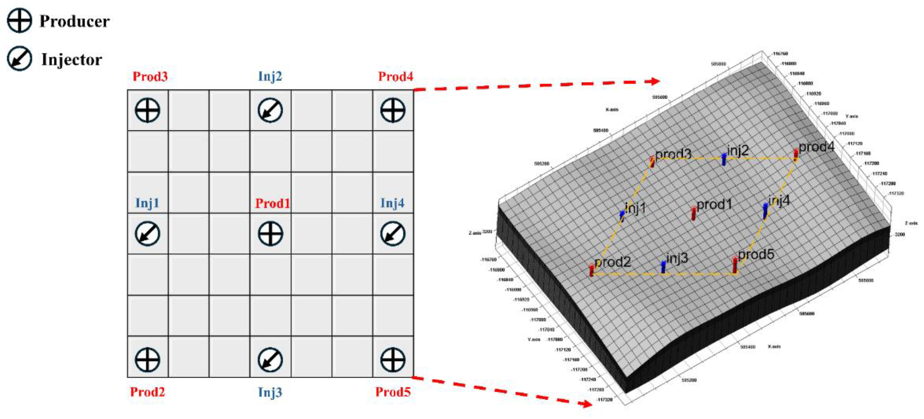
Figure 2.
Relative permeability curves for (a) Oil-Water systems and (b) Oil-Gas systems.
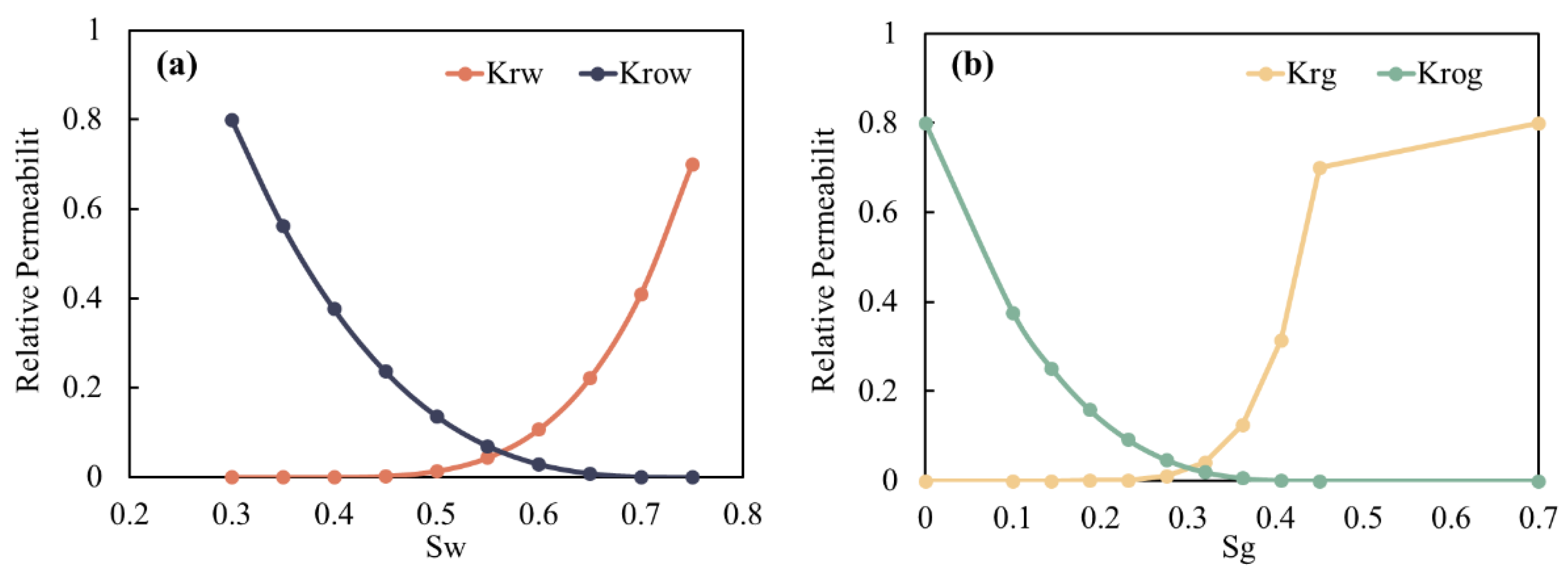
Figure 3.
Variable correlation and data normalization: (a) Pearson correlation heatmap; (b) Box plot of normalized variables.
Figure 3.
Variable correlation and data normalization: (a) Pearson correlation heatmap; (b) Box plot of normalized variables.
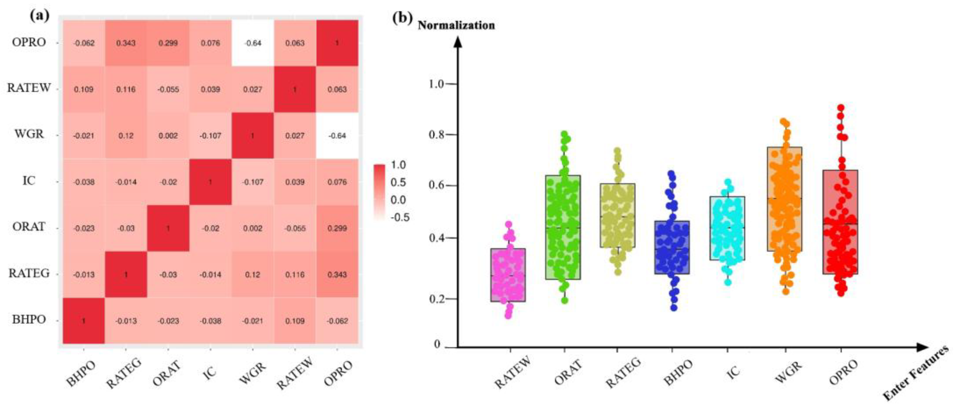
Figure 4.
Workflow of the CPO-XGBoost algorithm for hyperparameter optimization.
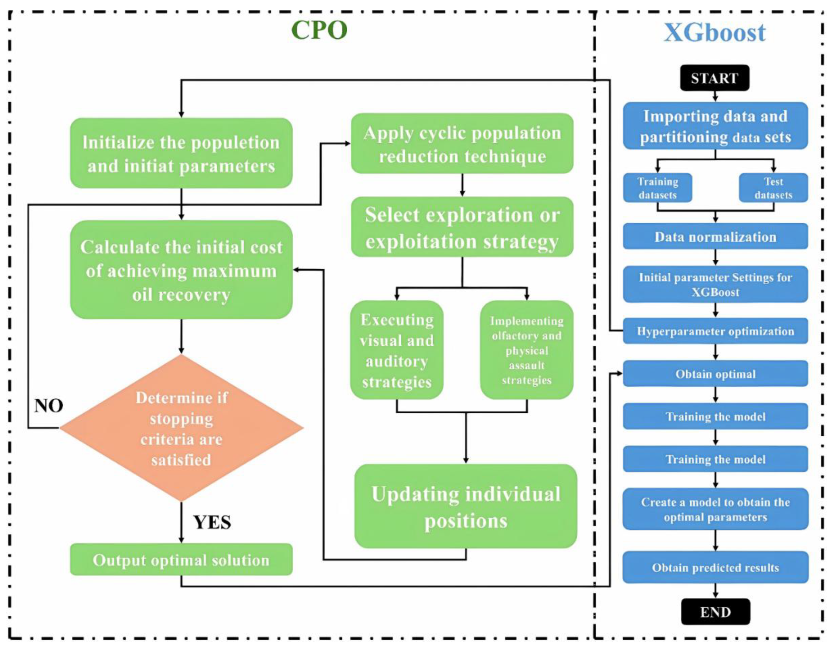
Figure 5.
Workflow of the GWO-XGBoost algorithm for hyperparameter optimization.
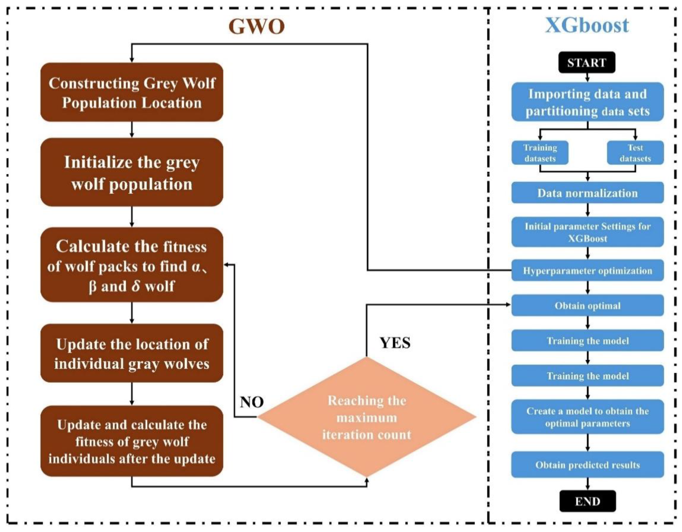
Figure 6.
Workflow of the AHA-XGBoost algorithm for hyperparameter optimization.
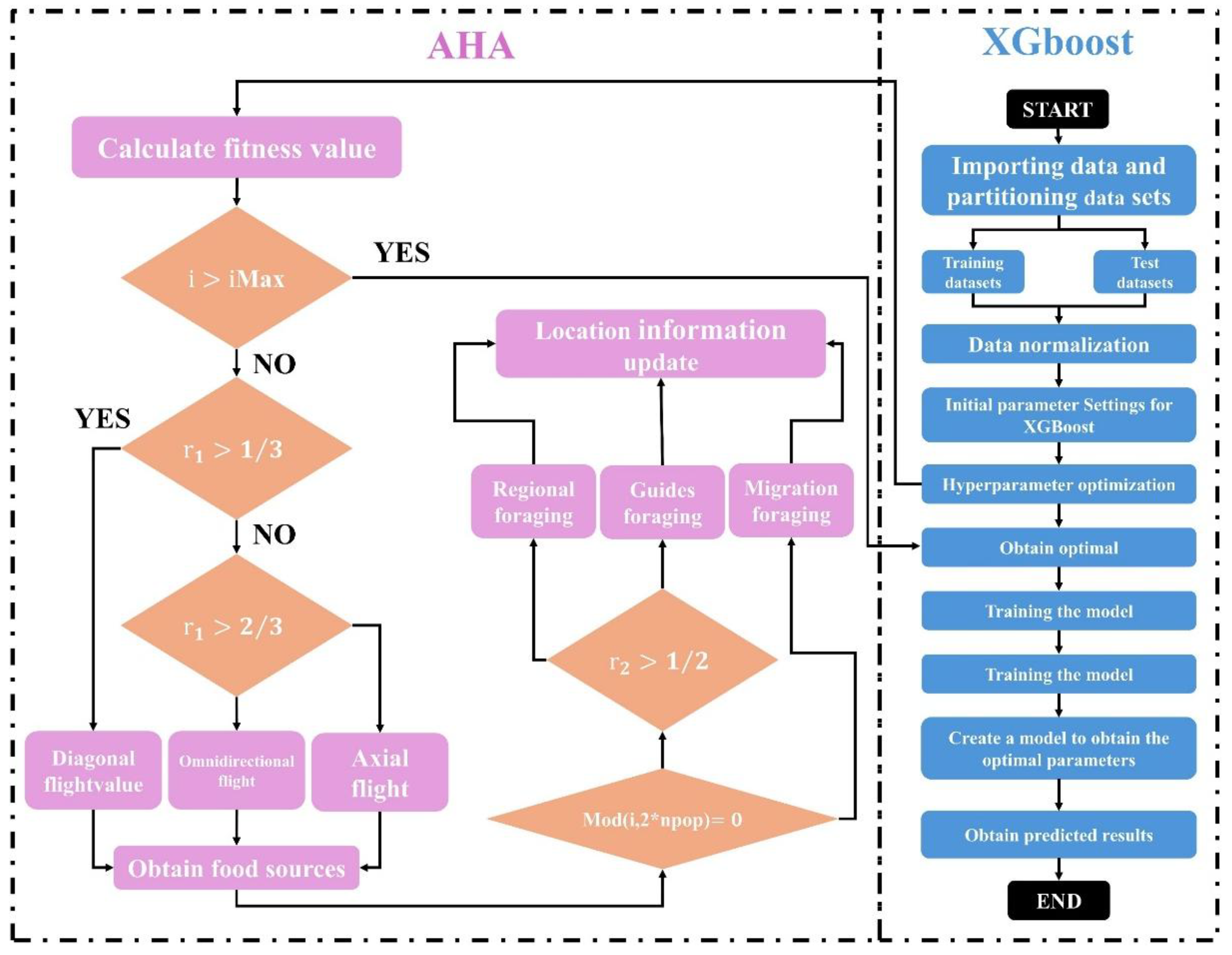
Figure 7.
Workflow of the BAK-XGBoost algorithm for hyperparameter optimization.
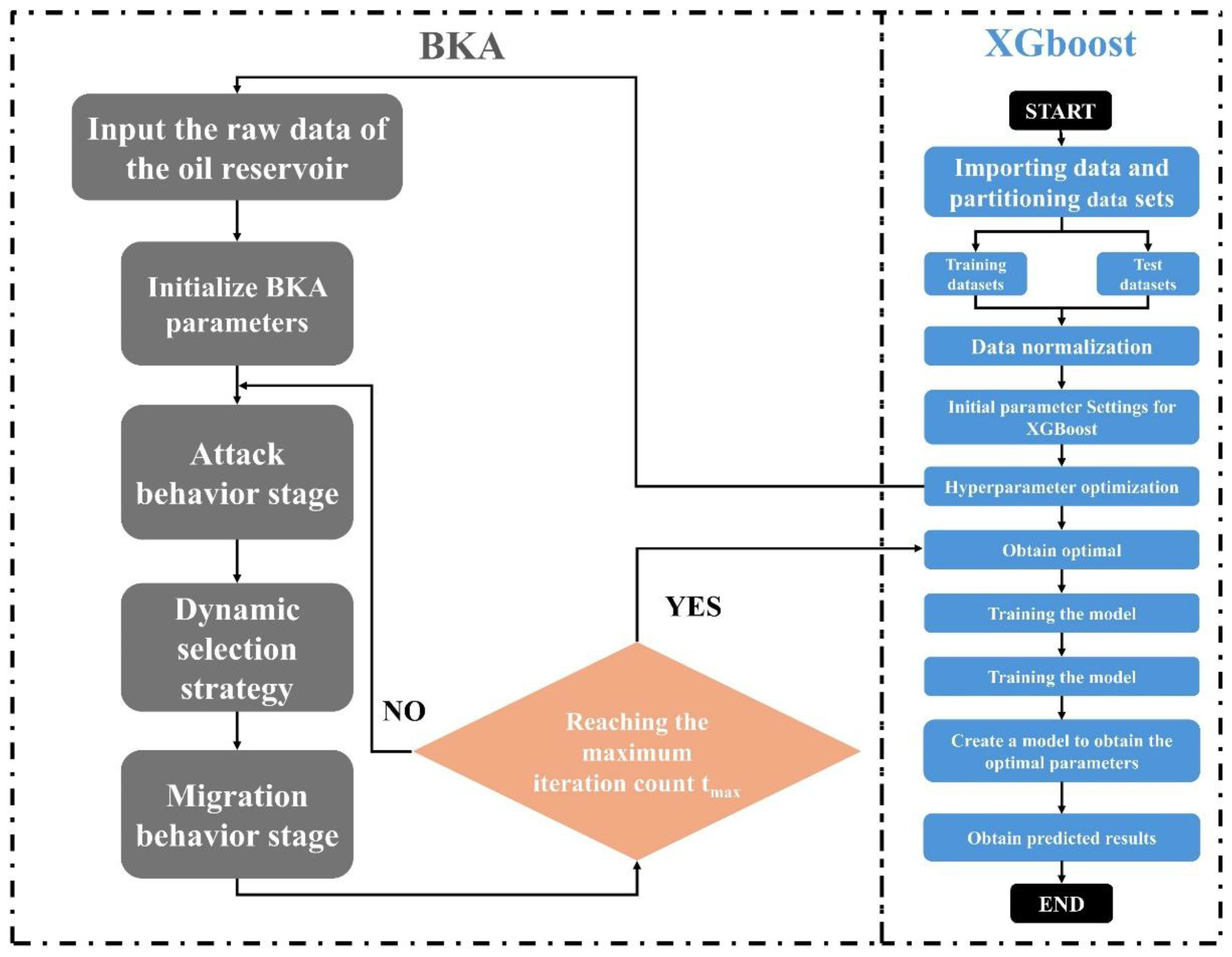
Figure 8.
The workflow of the ICPO-XGBoost algorithm.
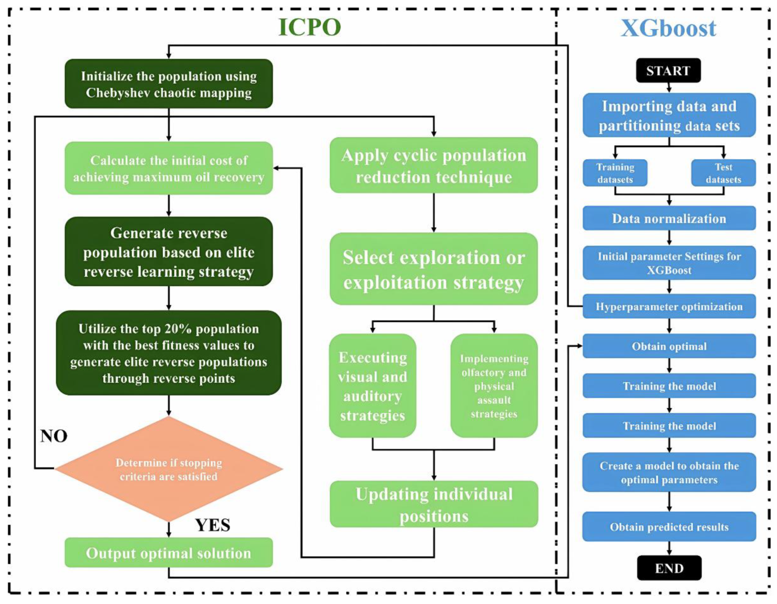
Figure 9.
Prediction values and error distributions of the six models.
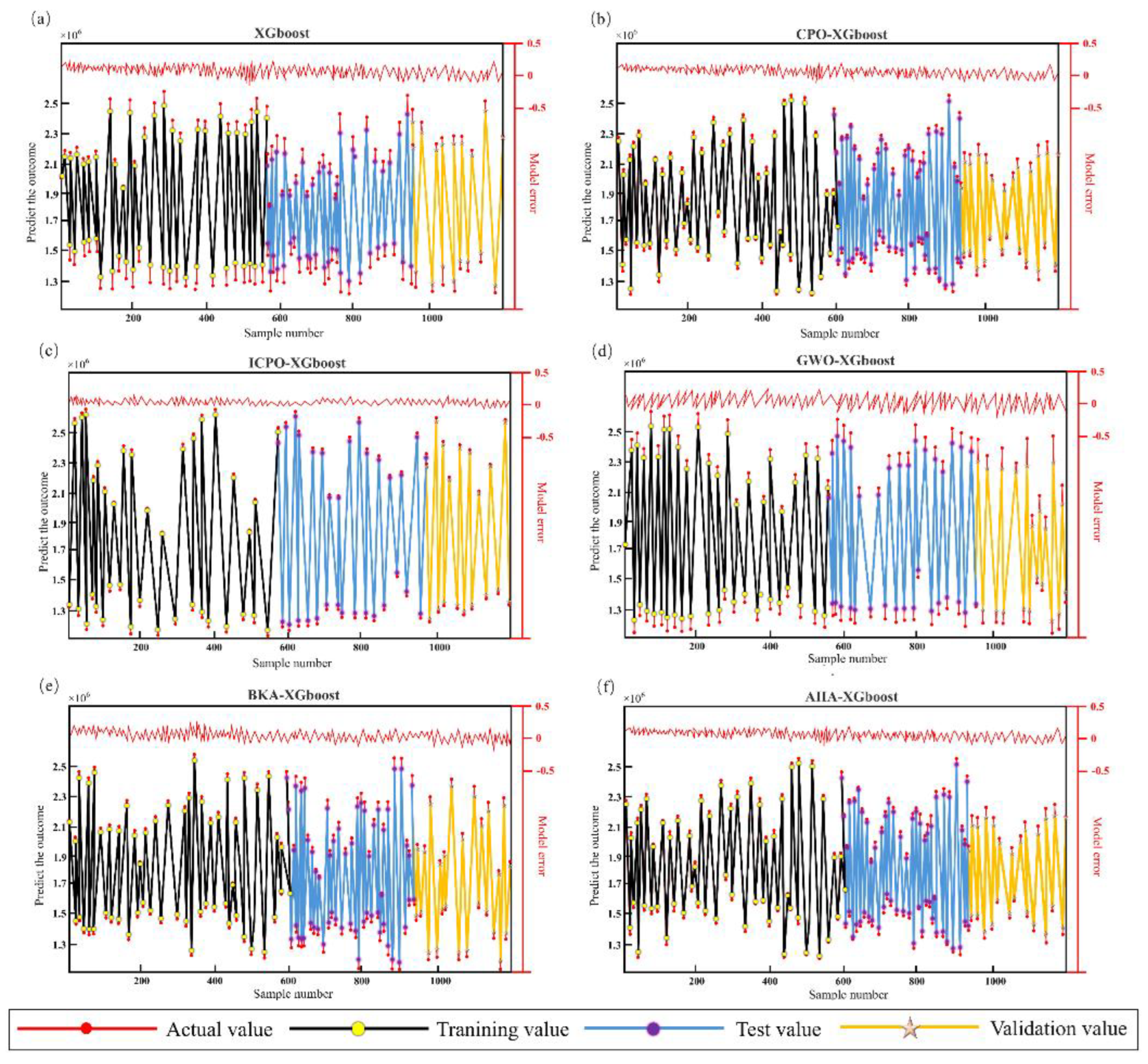
Figure 10.
Comparison between predicted and actual values for the four models.
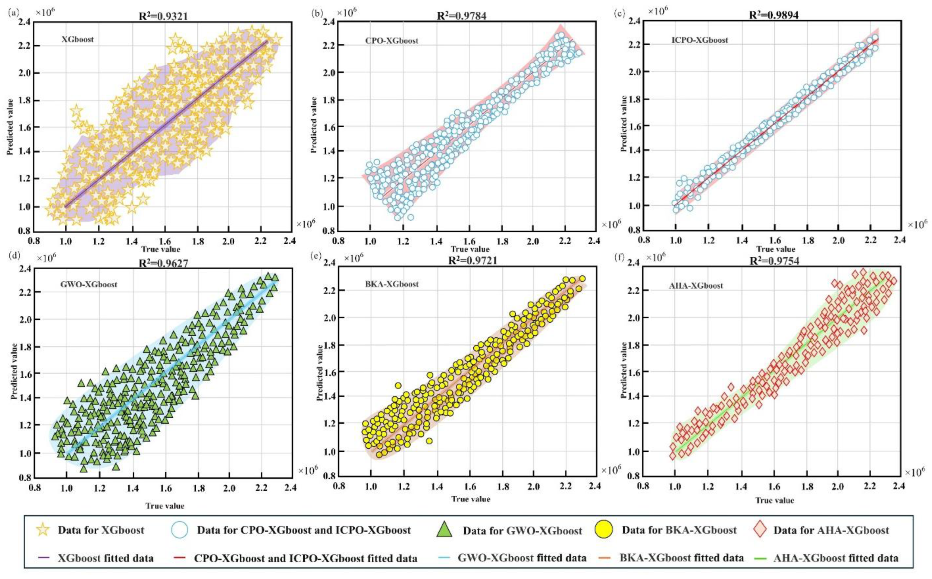
Figure 11.
Radar chart of evaluation metrics for the six models: (a) Training Set; (b) Testing Set; (c) Overall Data.
Figure 11.
Radar chart of evaluation metrics for the six models: (a) Training Set; (b) Testing Set; (c) Overall Data.
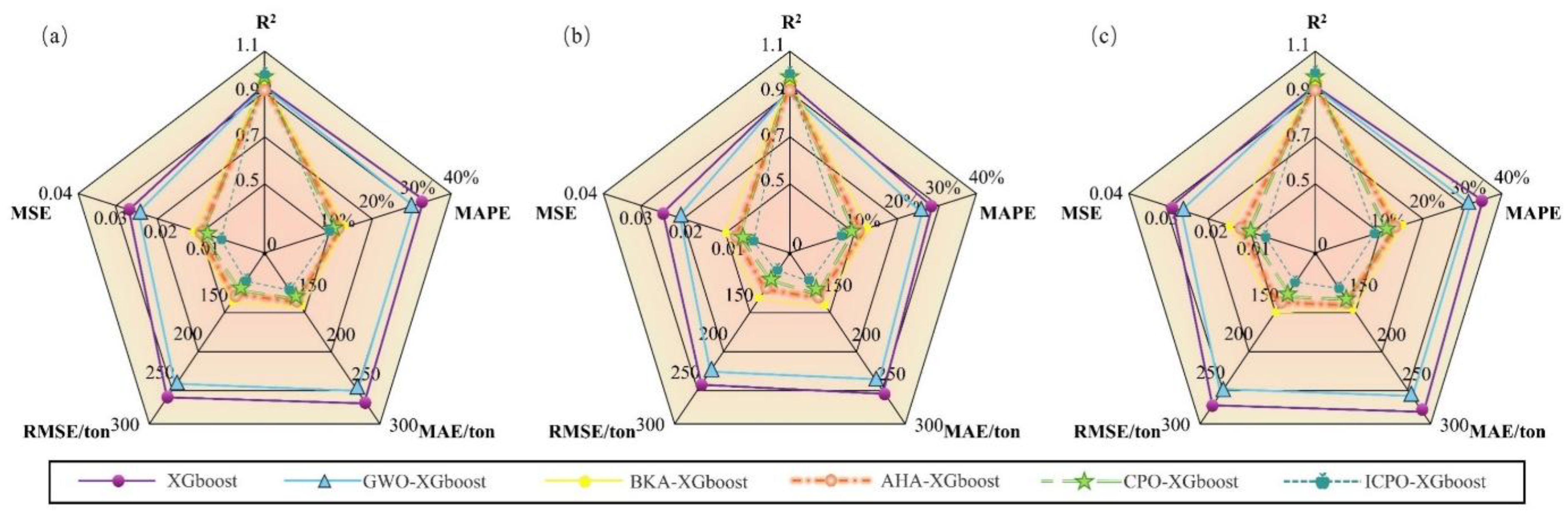
Figure 12.
Oil and gas saturation distribution for six development strategies at the 20-year production mark.
Figure 12.
Oil and gas saturation distribution for six development strategies at the 20-year production mark.
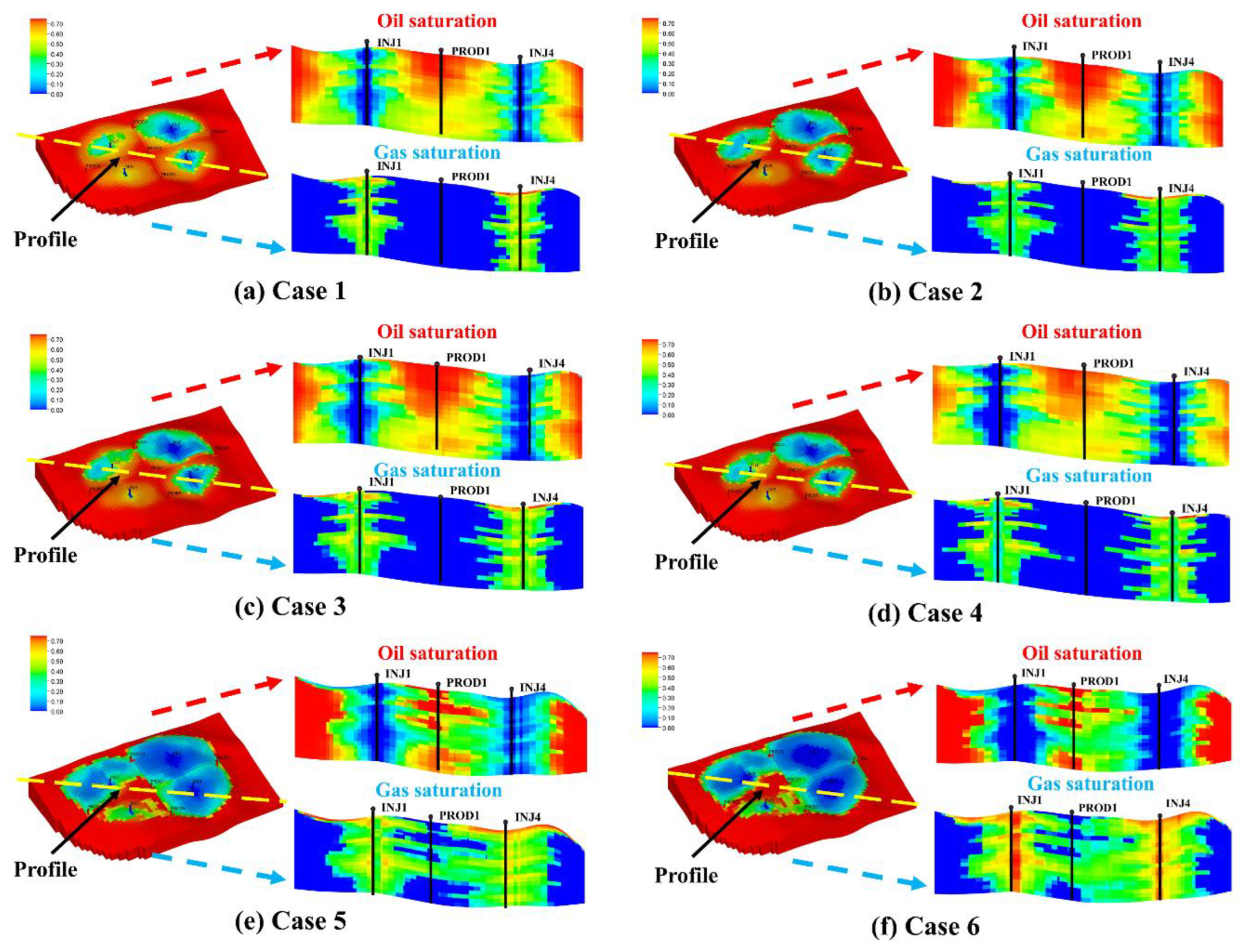
Figure 13.
(a) Comparison of predicted vs. simulated cumulative oil production; (b) Cumulative CO2 production and gas breakthrough analysis.
Figure 13.
(a) Comparison of predicted vs. simulated cumulative oil production; (b) Cumulative CO2 production and gas breakthrough analysis.
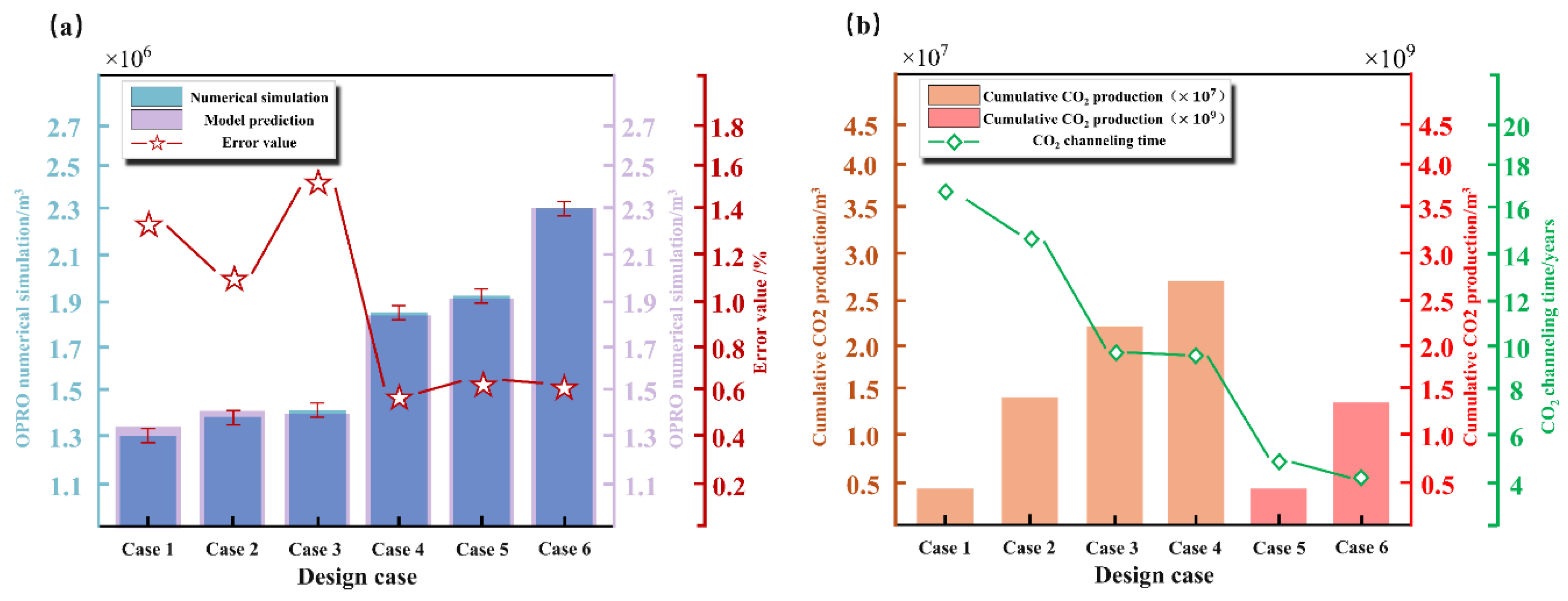
Figure 14.
SHAP analysis results: (a) Feature importance scores; (b) Feature impact on cumulative oil production.
Figure 14.
SHAP analysis results: (a) Feature importance scores; (b) Feature impact on cumulative oil production.
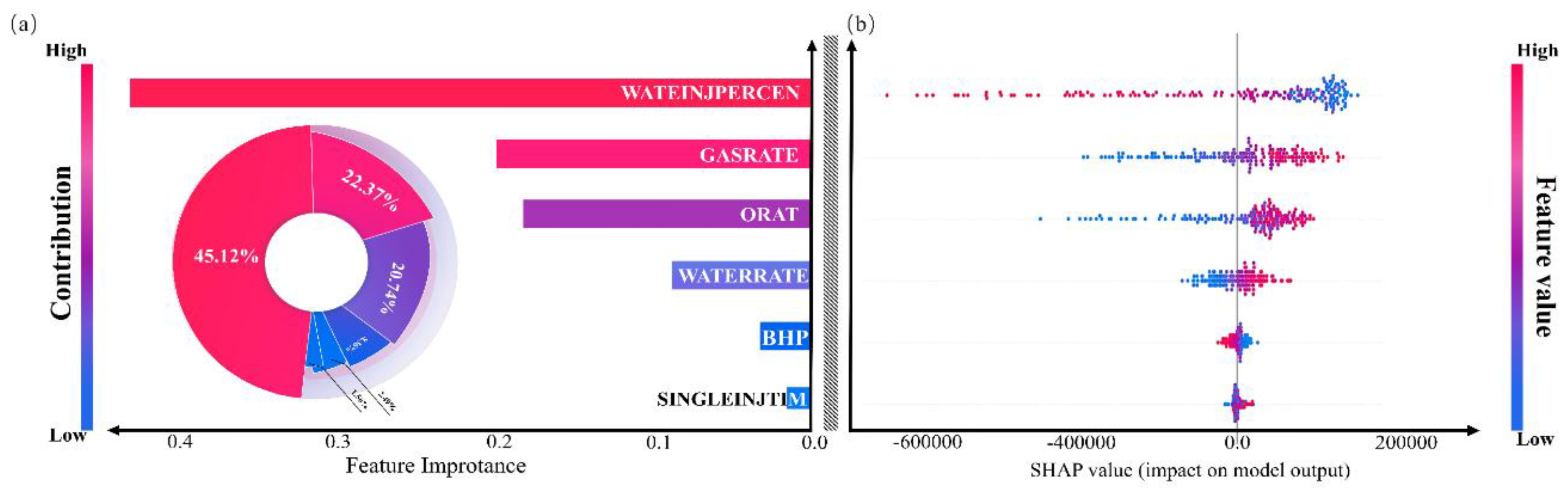

Table 1.
Compositional analysis of reservoir fluids.
| Components | Fraction | Components | Fraction |
|---|---|---|---|
| CO2 | 0.005 | C10+ | 0.115 |
| C1N2 | 0.253 | C12+ | 0.123 |
| C2+ | 0.083 | C16+ | 0.074 |
| C5+ | 0.112 | C20+ | 0.057 |
| C7+ | 0.178 |
Table 2.
Statistical summary of decision variables.
| Characteristic parameter | Unit | Mean | Maximum | Minimum | Standard deviation |
Skewness | Variable coefficient |
|---|---|---|---|---|---|---|---|
| BHPO | MPa | 17.4 | 20 | 15 | 1.45 | 0.0048 | 0.0826 |
| WGR | % | 50 | 90 | 10 | 30 | 0.0032 | 0.5778 |
| ORAT | m3/d | 65.1 | 90 | 40 | 14.4 | 0.0017 | 0.2212 |
| RATEG | m3/d | 34974.4 | 45000 | 25000 | 4440.5 | 0.0028 | 0.2887 |
| RATEW | m3/d | 46.1 | 60 | 30 | 8.7 | 0.0031 | 0.4972 |
| IC | Day | 106.9 | 150 | 60 | 53.9 | 0.0029 | 0.3849 |
| OPRO | m3 | 1757850.2 | 2354830.2 | 1019188.1 | 293397.1 | -0.2337 | 0.1671 |
Table 3.
Hyperparameter and training settings for the four optimized models.
| Model | Max learning rate | Learning rate | Warm-up rounds | Early stopping rounds | Sub-sample ratio |
Iteration count |
|---|---|---|---|---|---|---|
| XGBoost | 12 | 0.18 | 5 | 20 | 0.4 | 80 |
| CPO-XGboost | 14 | 0.21 | 8 | 25 | 0.5 | 140 |
| AHA-XGboost | 17 | 0.27 | 10 | 30 | 0.6 | 145 |
| BKA-XGboost | 15 | 0.29 | 10 | 30 | 0.4 | 125 |
| GWO-XGboost | 18 | 0.30 | 10 | 30 | 0.3 | 150 |
| ICPO-XGboost | 15 | 0.35 | 8 | 25 | 0.5 | 135 |
Table 4.
Primary evaluation metrics for the six models.
| Model | Data range | R2 | MAPE | MAE | RMSE | MSE |
|---|---|---|---|---|---|---|
| XGBoost | Training set | 0.9343 | 29.54% | 276.71 | 271.24 | 0.0285 |
| Test set | 0.9321 | 27.68% | 255.12 | 252.36 | 0.0242 | |
| Overall data | 0.9325 | 28.31% | 279.58 | 273.51 | 0.0277 | |
| CPO-XGboost | Training set | 0.9796 | 12.67% | 131.84 | 127.62 | 0.0095 |
| Test set | 0.9784 | 11.07% | 126.63 | 105.24 | 0.0074 | |
| Overall data | 0.9788 | 12.26% | 149.12 | 129.67 | 0.0081 | |
| ICPO-XGboost | Training set | 0.9902 | 10.21% | 119.92 | 95.53 | 0.0072 |
| Test set | 0.9894 | 8.47% | 112.65 | 67.94 | 0.0053 | |
| Overall data | 0.9896 | 9.87% | 125.63 | 102.98 | 0.0064 | |
| AHA-XGboost | Training set | 0.9749 | 16.52% | 148.15 | 135.15 | 0.0119 |
| Test set | 0.9721 | 15.94% | 142.92 | 114.28 | 0.0088 | |
| Overall data | 0.9725 | 16.42% | 151.45 | 142.61 | 0.0126 | |
| BKA-XGboost | Training set | 0.9768 | 14.62% | 141.51 | 132.82 | 0.0129 |
| Test set | 0.9754 | 14.28% | 138.87 | 125.95 | 0.0115 | |
| Overall data | 0.9758 | 14.59% | 142.12 | 136.08 | 0.0157 | |
| GWO-XGboost | Training set | 0.9632 | 28.42% | 252.81 | 245.34 | 0.0272 |
| Test set | 0.9627 | 27.33% | 248.92 | 238.26 | 0.0226 | |
| Overall data | 0.9629 | 28.15% | 256.22 | 245.58 | 0.0257 | |
| ICPO-XGboost | Training set | 0.9902 | 10.21% | 119.92 | 95.53 | 0.0072 |
| Test set | 0.9894 | 8.47% | 112.65 | 67.94 | 0.0053 | |
| Overall data | 0.9896 | 9.87% | 125.63 | 102.98 | 0.0064 |
Table 5.
Parameters and results of six development strategies.
| Parameter | Unit | Case1 | Case2 | Case3 | Case4 | Case5 | Case6 |
|---|---|---|---|---|---|---|---|
| BHPO | MPa | 18.5 | 17.3 | 18.4 | 17.6 | 17.5 | 16.6 |
| WGR | % | 30 | 85 | 87 | 90 | 45 | 90 |
| ORAT | m3/d | 82.73 | 89.85 | 42.01 | 44.85 | 78.45 | 82.73 |
| RATEG | m3/d | 29940.96 | 38116.19 | 39678.19 | 33328.05 | 38912.61 | 39940.96 |
| RATEW | m3/d | 45.38 | 41.47 | 41.16 | 56.77 | 51.04 | 52.35 |
| IC | Day | 122.27 | 184.55 | 106.01 | 61.52 | 113.28 | 82.27 |
| Simulation prediction | ×106m3 | 1.308 | 1.348 | 1.424 | 1.495 | 1.881 | 2.355 |
| Model prediction | ×106m3 | 1.311 | 1.349 | 1.421 | 1.494 | 1.881 | 2.355 |
Disclaimer/Publisher’s Note: The statements, opinions and data contained in all publications are solely those of the individual author(s) and contributor(s) and not of MDPI and/or the editor(s). MDPI and/or the editor(s) disclaim responsibility for any injury to people or property resulting from any ideas, methods, instructions or products referred to in the content. |
© 2025 by the authors. Licensee MDPI, Basel, Switzerland. This article is an open access article distributed under the terms and conditions of the Creative Commons Attribution (CC BY) license (http://creativecommons.org/licenses/by/4.0/).
Copyright: This open access article is published under a Creative Commons CC BY 4.0 license, which permit the free download, distribution, and reuse, provided that the author and preprint are cited in any reuse.


