Submitted:
29 June 2025
Posted:
08 July 2025
You are already at the latest version
Abstract
This study explores the use of deep learning techniques for classifying EEG signals in the context of Alzheimer’s disease (AD) and frontotemporal dementia (FTD). We propose a novel classification pipeline that combines autoencoders for feature extraction and bidirectional long short-term memory (Bi-LSTM) networks for temporal analysis of EEG data. Given the challenges of processing high dimensional EEG signals, we employed an Autoencoder to reduce the data’s dimensionality while preserving key features relevant for diagnosis. The Bi-LSTM model effectively captured the temporal dependencies in the EEG signals, essen- tial for detecting subtle neural changes indicative of AD and FTD. Furthermore, we leveraged SHapley Additive exPlanations (SHAP) to interpret the model’s predictions, providing transparency and ensuring that the contributions of individual features in the decision-making process are understood. The results demonstrate the efficacy of this approach, achieving an accuracy of 98%, while maintaining interpretability, making it a promising tool for clinical applications in the diagnosis of neurodegenerative diseases.
Keywords:
EEG
; Deep learning
; Multimodal fusion
; Real-time systems
; Hybrid neural networks
; SHAP explainability
; DEAP dataset
; Cognitive monitoring
; Alzheimer’s disease
; frontotemporal dementia
; Neurodegenerative disease detection
; Autoencoder
; Bidirectional LSTM (Bi-LSTM)
; Explainable AI (XAI)
; Feature extraction
; EEG signal analysis
1. Introduction
Our brain is a complex system consisting of approximately 100 billion neurons, interconnected through a complicated neural network. The term neurodegenerative refers to the damage or death of these neurons [1,2].
The frequency of discussions around neurodegenerative diseases, such as Alzheimer’s disease and frontotemporal dementia, has been increasing in recent years. These disorders, closely related to brain neuronal degeneration, have a profound impact on cognitive function, memory, and behavior. Alzheimer’s disease is one of the famous neurodegenerative diseases, it causes mainly memory loss, and is common among older people; today more than 50 million people have Alzheimer around the world [3,4]. On the same note, Frontotemporal Dementia is a neurodegenerative disorder that affects mainly the frontal and temporal lobes of the brain. These areas of the brain are associated with personality, behavior, and language; it tends to occur at a younger age than Alzheimer’s disease. It often begins between the ages of 40 and 65 [5]. To this day, there is no known cure for these diseases. Treatments for Alzheimer’s focus primarily on slowing the progression of symptoms. For FTD, the challenge is even greater; There are no approved treatments to slow, stop, or cure the disease. Therefore, the demand for an early and accurate diagnosis becomes more urgent. That’s the motivation behind our research [6,7].
Current diagnostic methods like physical exams and brain scans often fail to capture the subtle and dynamic brain activities crucial for understanding the progression of dementia and its early signs [8]. EEG, or electroencephalogram, has made significant strides in capturing brain signals. Due to its non-invasive nature, EEG measures the brain’s electrical activity through electrodes placed on the scalp, providing valuable insights into brain changes associated with Alzheimer and FTD’s disease [2]. However, the volume of recorded EEG data and artifacts are a challenge in extracting valuable features, and thus, accurately diagnosing neurodegenerative diseases [4]. The application of machine learning techniques to classify EEG signals is an expanding field of research. These techniques have the potential to analyze vast amounts of EEG data, identify patterns, and potentially aid in the early diagnosis of neurodegenerative disorders. However, the success of this approach relies on several critical factors: selecting the right EEG dataset, accurately identifying relevant features, choosing the most suitable algorithm, and rigorously evaluating its performance to ensure the reliability and integrity of the results [4].
This research aims to leverage deep learning techniques to analyze EEG signals, identifying patterns that can aid in the detection and diagnosis of Alzheimer’s Disease and frontotemporal dementia. Our primary objective is to accurately identify and extract relevant features from EEG signal. To achieve that we adopted the Hybrid Approach of Auto-encoder and LSTM. Additionally, we incorporated explain-ability into our model results through explainable AI (XAI) techniques, providing an understanding of how the model make predictions.
The remainder of this paper is structured as follows: Section 2 surveys existing literature on EEG-based detection of neurodegenerative disorders, emphasizing methodological limitations in feature selection and model interpretability. Section 3 describes the dataset characteristics, preprocessing methodology (including signal segmentation and standardization), and feature extraction techniques, with a focus on Power Spectral Density (PSD) and Autoencoder-derived dimensionality reduction. Section 4 introduces the proposed hybrid architecture, integrating Autoencoders with Bidirectional Long Short-Term Memory (Bi-LSTM) networks, and outlines the SHapley Additive exPlanations (SHAP) framework for explainability. Section 5 evaluates experimental results, benchmarking model performance against baseline classifiers and analyzing the influence of temporal windowing on accuracy, supported by SHAP-based feature importance quantification. The paper concludes with Section 6, which summarizes key findings, acknowledges current limitations in whole-signal processing, and proposes future directions for clinical deployment and real-time analysis.
The code and resources for this project are publicly available on GitHub at .
2. Related Works
The study of EEG-based diagnosis for neurodegenerative diseases particularly Alzheimer’s Disease (AD) and frontotemporal dementia (FTD) has gained a lot of attention in recent years. Many researchers have explored the potential of EEG signals and machine learning techniques for the early detection and classification of these disorders.
This Study [4], utilized Singular Value Decomposition (SVD) entropy as the core feature extraction technique to identify biomarkers from EEG signals. This method effectively isolated relevant patterns associated with Alzheimer’s disease (AD) and frontotemporal dementia (FTD). The integration of SVD entropy into the framework allowed for the precise extraction of EEG characteristics, which were then input into a K-Nearest Neighbors (KNN) classifier. By combining sliding window analysis with this approach, the researchers enhanced the model’s ability to capture temporal dynamics, resulting in high accuracy and F1-scores across classification tasks. The study also explored other feature extraction techniques, including power spectral density and wavelet transform, to evaluate their efficacy in capturing EEG signal characteristics. In terms of classification models, methods such as Support Vector Machines (SVM), Random Forest, and Neural Networks were assessed. Among these, the combination of SVD entropy for feature extraction and K-Nearest Neighbors (KNN) emerged as the most effective, achieving the highest classification metrics, with an accuracy of up to 93 in distinguishing between AD, FTD, and healthy controls (HCs). This demonstrates the robustness of their selected approach.
Similarly, this research [5] focused on feature extraction, they calculated power spectral densities (PSDs) across key frequency bands—Delta, Theta, Alpha, Beta, and Gamma; providing a detailed representation of signal frequency components. These PSDs and their relative ratios served as the core features for model training. Five machine learning classifiers were implemented: k-Nearest Neighbors (k-NN), Support Vector Machines (SVM), Random Forests, Neural Networks, and Naive Bayes. Among these, Random Forests performed the best, demonstrating the highest accuracy in distinguishing the three diagnostic groups. The study also employed leave-one-out cross-validation to ensure robust model evaluation. This work underscores the importance of selecting appropriate features and classification models, offering valuable insights and a benchmark dataset for advancing EEG-based diagnostic methods.
Likewise, many researches focused mainly on features extraction from EEG signals, some have employed entropy-based features [6], which are mathematical measures used to quantify the complexity, randomness, or predictability of EEG signals. They provide insights into the underlying brain dynamics and are particularly useful in distinguishing between healthy and pathological states, such as neurodegenerative disorders or epilepsy. Some used Hjorth parameter [7], those are three statistical measures—Activity, Mobility, and Complexity—used in EEG signal analysis to quantify the signal’s characteristics in both the time and frequency domains.
On the same note, many researches adopted machine and deep learning in their approaches [8,9,10]. This research focused on using CNN, and it was trained to focus on brain connectivity features for AD detection [11]. Others explored the role of advanced machine learning techniques in analyzing EEG data for detecting neurodegenerative diseases, using LSTM (Long Short-Term Memory) networks, which are effective at handling sequential data like EEG signals, the study achieved high classification accuracy [12].
Research on detecting Alzheimer’s disease and frontotemporal dementia using EEG data is comprehensive, with significant progress in applying machine learning and deep learning to enhance predictive accuracy. Yet, a challenge remains: assessing the effectiveness of different interpretable methods for identifying critical features in EEG data related to these disorders. These features often serve as key inputs for the predictive models but remain difficult to accurately evaluate, leaving room for further exploration in understanding their true potential.
3. Methods and Materials
3.1. Dataset Overview
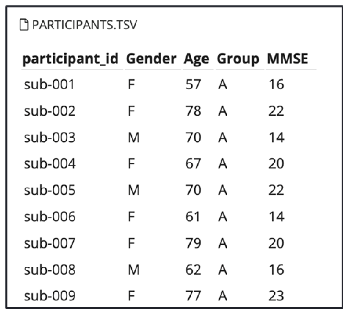
In this study, we utilized a publicly available EEG dataset provided by OpenNeuro, titled “A dataset of EEG recordings from Alzheimer’s Disease, Frontotemporal Dementia, and Healthy Subjects” [18]. This dataset comprises EEG recordings collected during the resting state with eyes closed, from elderly patients diagnosed with Alzheimer’s disease (AD) and frontotemporal dementia (FTD), as well as healthy age-matched controls (CN). The dataset includes recordings from 88 participants with information about their Gender and Age as shown in Figure 5. Among the total of participants : 36 individuals with Alzheimer’s disease (AD group), 23 with frontotemporal dementia (FTD group), and 29 cognitively normal controls (CN group).
Figure 1.
Participants Information
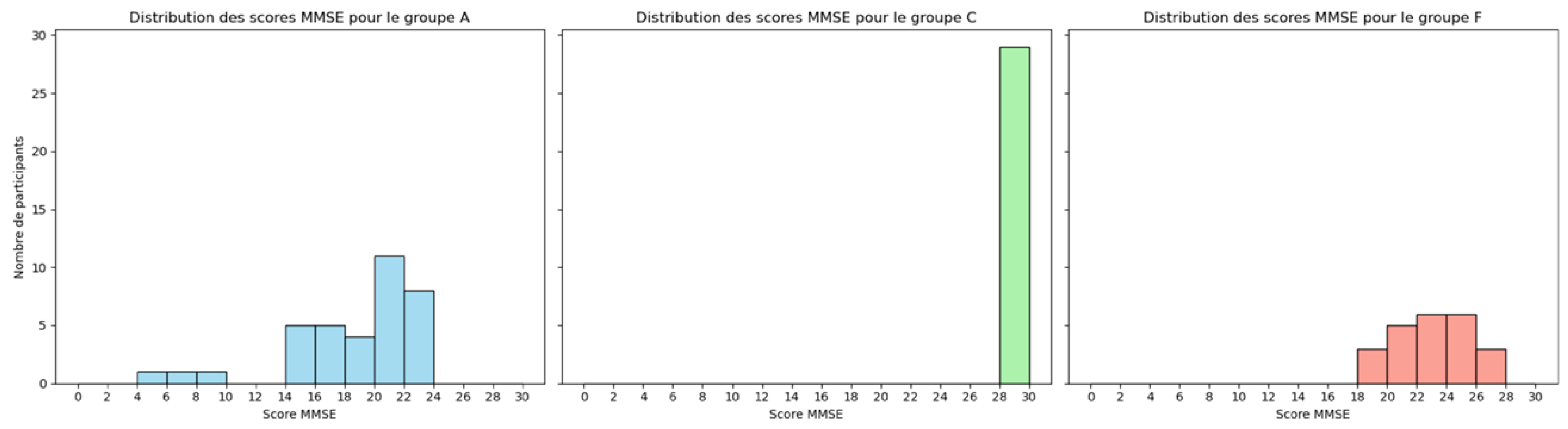
Cognitive and neuropsychological assessments were conducted using the international Mini-Mental State Examination (MMSE), a widely recognized tool for measuring cognitive impairment. The MMSE score ranges from 0 to 30, with lower scores indicating greater cognitive decline. The lower MMSE score usually aligns with participants who have AD and FTD, as shown in the Figure 5 [19].
Figure 2.
Participants MMSE Scores in the Tree Groups : AD, FTD and CN
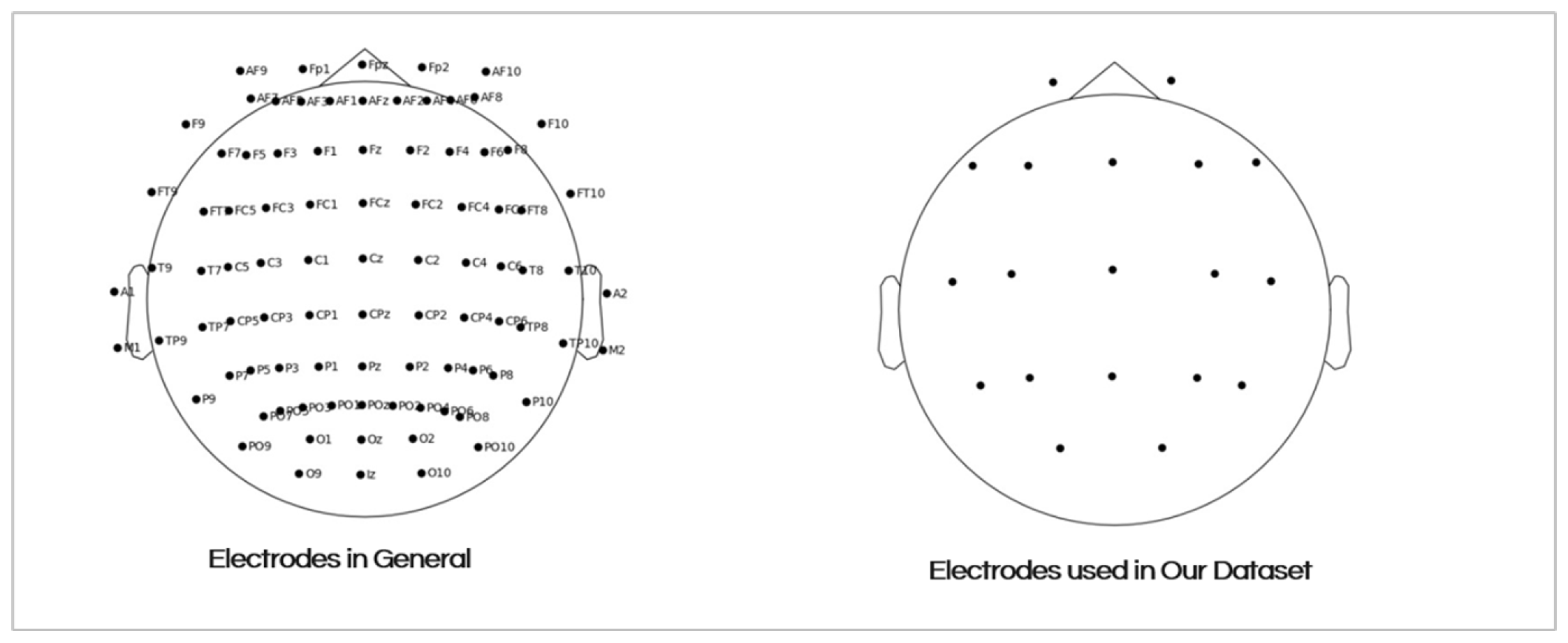
The EEG signals were recorded from 19 scalp electrodes (Fp1, Fp2, F7, F3, Fz, F4, F8, T3, C3, Cz, C4, T4, T5, P3, Pz, P4, T6, 01, and O2) using a standardized 10-20 electrode placement system. The Figure 5 shows the placement of the electrodes on the scalp. The recording durations varied between groups:
- AD group: Mean duration of 13.5 minutes (min = 5.1, max = 21.3)
- FTD group:Mean duration of 12 minutes (min = 7.9, max = 16.9)
- CN group: Mean duration of 13.8 minutes (min = 12.5, max = 16.5)
In total, the dataset includes approximately 485.5 minutes of AD recordings, 276.5 minutes of FTD recordings, and 402 minutes of CN recordings. This rich dataset provides a comprehensive basis for exploring the differences in brain activity among these diagnostic groups, contributing valuable insights into the neurophysiological signatures of cognitive disorders [18].
Figure 3.
The 19 Electrodes Placement on the Scalp
3.2. Signal Preprocessing and Feature Extraction
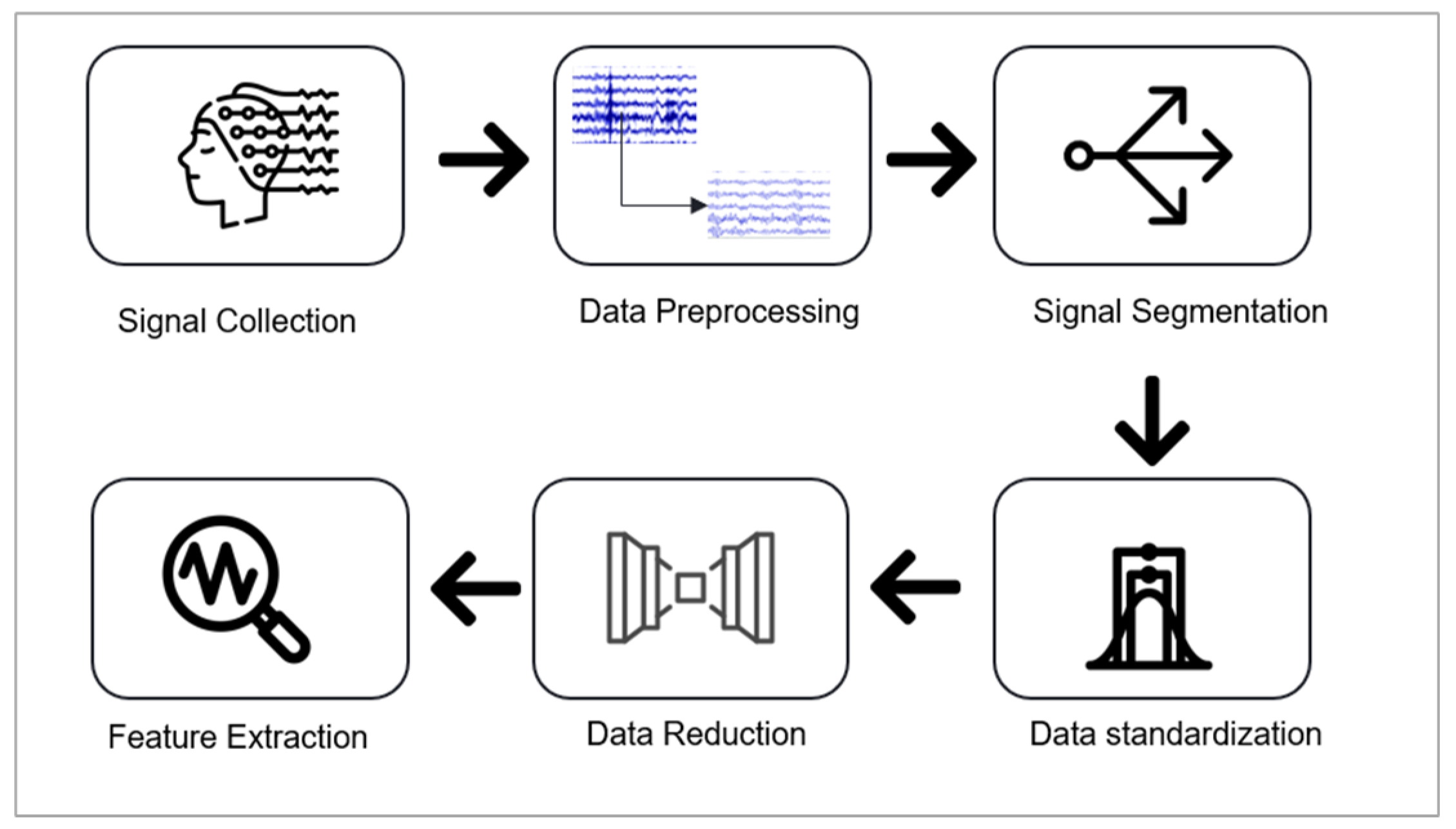
In the preprocessing and feature extraction stage, the following pipeline was implemented: data preprocessing, data segmentation and standardization, application of an autoencoder for dimensionality reduction, and feature extraction. Figure 5 illustrates these steps, which are are explained in detail below.
Figure 4.
Preprocessing and Feature Extraction Pipeline
3.2.1. Data Preprocssing
For Preprocessing, We used the EEG data that had already been preprocessed by OpenNeuro. The preprocessing pipeline applied by OpenNeuro included several key steps to ensure high-quality data for analysis. The signals were re-referenced to the average value of the A1-A2 channels and underwent a Butterworth band-pass filter (0.5–45 Hz) to remove low-frequency drift and high-frequency noise. The data was also processed using the Automatic Source Reconstruction (ASR) routine, which eliminated large-amplitude or persistent artifacts by rejecting data periods with a standard deviation exceeding 17 over a 0.5-second window. Additionally, Independent Component Analysis (ICA) was performed to decompose the EEG channels into independent components, and components identified as “eye” or “jaw” artifacts by the ICLabel tool were excluded. These preprocessing steps, already performed by OpenNeuro, ensured that the dataset was clean and artifact-free for subsequent analysis.
3.2.2. Signal Segmentation
In this research, the EEG signal recordings are relatively long, with a maximum duration of 21.3 minutes, which poses challenges for feature extraction when processing the entire signal. To address this, window sliding is applied to segment the signal into manageable portions.
In the context of AD and FTD, studies on EEG typically employ shorter epochs for tasks that aim to analyze fast cognitive responses, like detecting changes in attention, working memory, or sensory processing. These are mostly suitable for observing cognitive deficits during specific mental tasks [13]. However, there is no consensus on this matter. It is essential to test different window length ranges to identify the optimal result[14]. In this study, we tested various intervals ranging from 3 seconds to 12 seconds. The results of this test will be presented in the results section. In this study, a window length of 5 seconds with a 50% overlap was used.
3.2.3. Data Standardization
In the context of this pipeline, data standardization plays a crucial role in ensuring the consistency and comparability of features extracted from EEG signals. Standardization scales the data to have a mean of zero and a standard deviation of one, which is particularly important for EEG signal processing due to the variability in amplitude and frequency ranges across recordings. This step helps prevent biases during feature extraction and ensures that the model learn patterns relevant to the task, rather than being influenced by scale differences in the input data.
In our approach, standardization is employed to normalize the EEG signals, making them suitable for downstream processes. Each segment of the EEG signals was standardized independently across channels. This standardization procedure was applied to all data segments to ensure that each channel contributed equally to the model’s learning process.
3.2.4. Data Reduction
In our feature extraction approach, we leveraged an autoencoder for dimensionality reduction, a widely recognized method for learning compact and meaningful representations of data. Autoencoders [22] are neural networks trained to encode input data into a compressed latent space and subsequently decode it back into its original form, Figure 5 illustrates its architecture. This process encourages the model to capture the most salient features while discarding noise and redundant information, making it highly effective for dimensionality reduction and feature extraction [23].
Figure 5.
Bi-Directional LSTM Architecture
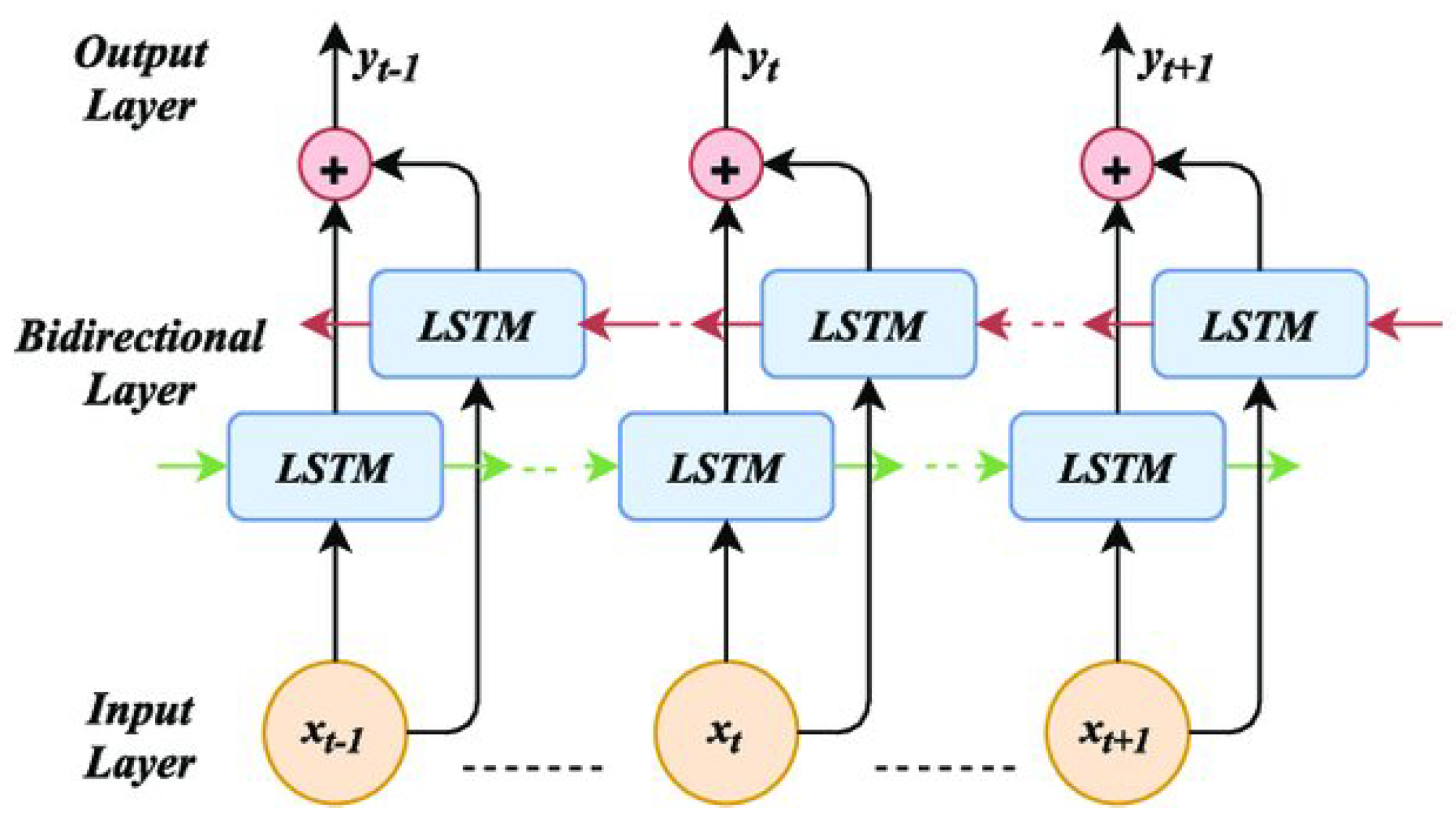
The autoencoder consists of two main components: the encoder and the decoder. The encoder compresses the input data into a low-dimensional latent representation, capturing the underlying patterns and correlations. The decoder reconstructs the original data from this representation, ensuring that the compressed features retain essential information. During training, the autoencoder minimizes reconstruction error, effectively learning a compact and noise-robust representation of the input.
In our study, a neural network-based autoencoder was trained on standardized EEG segments. The encoder component was specifically designed to capture lower-dimensional representations of the signals, preserving essential characteristics indicative of neurological conditions. The compressed features generated by the encoder were subsequently used as inputs for downstream analysis and classification tasks. This approach not only reduced the computational complexity of the model but also improved its ability to identify subtle patterns associated with AD and FTD, enhancing diagnostic accuracy.
After applying the Autoencoder for dimensionality reduction, the next step in our pipeline is to extract meaningful features from the compressed representation of the EEG signals. These features serve as the core inputs for subsequent classification tasks, capturing critical information about the underlying patterns in the brain activity.
3.2.5. Feature Extraction
EEG signals provide a variety of features that can be exploited for neurological studies. In our research, we focused on the Power Spectral Density (PSD) feature, which is widely recognized for its use in EEG-related studies and analyses [15,16]. PSD is a signal processing method that characterizes the variations in power (or energy) across different frequencies within a time series. The PSD can be calculated using techniques such as Fast Fourier Transform (FFT) or Autocorrelation Function [17].
In our study, we used the PSD method to decompose the EEG signals into distinct frequency bands that represent different brain activity states. These bands include:
- Delta:(1–4 Hz)
- Theta:(4–8 Hz)
- Alpha: (8–13 Hz)
- Beta: (13–30 Hz)
- Gamma: (30–60 Hz)
A growing body of literature has shown that PSD is correlated with various neurodegenerative diseases, including Alzheimer’s Disease (AD) and Frontotemporal Dementia (FTD) [17,18]. Specifically, dementia patients exhibit increased low-frequency activity in the Delta and Theta bands, which reflects the slowing of brain activity, a characteristic feature of cognitive decline and neuronal dysfunction in these conditions. Additionally, there is a reduction in higher-frequency power in the Alpha, Beta, and Gamma bands, which is commonly observed in dementia patients. These decreases are associated with impairments in cognitive functions such as attention, memory, and executive processing.
In addition to PSD, Singular Value Decomposition (SVD) Entropy has been explored as another important feature for analyzing EEG data. SVD Entropy quantifies the complexity of the EEG signal and is useful for capturing subtle changes in brain dynamics that may be linked to neurodegenerative diseases. Recent studies have shown that the entropy derived from SVD can distinguish between healthy controls and patients with Alzheimer’s disease or Frontotemporal Dementia by reflecting alterations in brain network connectivity and the degree of disorder in brain activity patterns [4].
After Applying Autoencoder we extracted the Power Spectral Density features (PSD). To calculate PSD for the time-windowed epochs, we utilized the Welch method. The Welch method is widely used due to its computational efficiency, as it employs the Fast Fourier Transform (FFT) for estimating the power spectrum. This method divides the signal into overlapping segments and computes the squared magnitude of the discrete Fourier transform for each segment. The final PSD estimate is then obtained by averaging the values from all segments, reducing variance and increasing the reliability of the spectral estimate [18]. Finally, we calculated spectral entropy from the extracted power bands. The entropy was computed by normalizing the power within each band, followed by the application of the Shannon entropy formula to quantify the degree of randomness in the frequency distribution for each epoch.
4. Implemented Approaches
4.1. Machine Learning Models
In the initial experiments, we employed classical algorithms such as K-Nearest Neighbors (KNN) and Support Vector Machines (SVM). However, the results were not satisfactory, underscoring the necessity for more advanced and sophisticated techniques.
4.1.1. K-Nearest Neighbors (KNN)
KNN is a simple, yet effective, instance-based learning algorithm that makes predictions based on the class of the nearest data points in the feature space. The primary idea behind KNN is that similar data points tend to have similar outcomes (or labels). The algorithm classifies a data point by looking at the ’k’ closest labeled points in the feature space and assigning the majority class label among those nearest neighbors [19] . The value of ’k’ plays a crucial role in determining the algorithm’s performance—if ’k’ is too small, the model may be sensitive to noise, while a large ’k’ may smooth over the classification boundaries [20]. Despite its simplicity, KNN struggles with high-dimensional data, such as EEG signals, where the curse of dimensionality may lead to reduced effectiveness.
4.1.2. Support Vector Machines (SVM)
SVM is a supervised learning algorithm that works by finding the hyperplane that best separates the data points from different classes with the maximum margin. The margin is defined as the distance between the hyperplane and the closest data points from each class, called support vectors [21]. SVM is particularly effective in high-dimensional spaces, making it well-suited for EEG signal classification, where the features can be numerous and complex. One of the key advantages of SVM is its ability to handle non-linear classification tasks by using the kernel trick, which transforms the feature space into a higher-dimensional space where linear separation is possible . However, SVM can be computationally intensive, particularly when dealing with large datasets or a high number of features, and may require careful tuning of hyperparameters, such as the choice of the kernel and regularization parameters, to avoid overfitting [22].
Despite the theoretical strengths of KNN and SVM, their performance on our EEG-based disease detection task was suboptimal, highlighting the need for more robust and adaptable models to handle the intricacies and high-dimensionality of EEG data.
4.2. Deep Learning Architectures
The methodology proposed for our classification approach leverages deep learning techniques [32]. In recent decades, EEG data has been extensively applied in data analysis methods, particularly time series analysis. With the significant advancements in deep learning (DL) for time series data, numerous studies have begun applying DL algorithms to the processing of EEG signals [33].
In this study, we combined two key components: an Autoencoder and the Long Short-Term Memory (LSTM) [34] network. The Autoencoder is a type of neural network designed to learn efficient codings of input data, typically for the purpose of dimensionality reduction. It consists of an encoder that compresses the high-dimensional EEG signals into a lower-dimensional latent space and a decoder that reconstructs the original data from this representation. This allows the Autoencoder to capture the essential features in EEG data while discarding redundant information [23]. The compressed representation retains the most important features for classification, which improves the efficiency and accuracy of the subsequent model.
Following this, the LSTM model is applied to analyze the temporal dependencies in the EEG data, which is crucial for detecting subtle changes in neural activity over time. LSTMs are a specialized type of Recurrent Neural Network (RNN) designed to address the vanishing gradient problem in traditional RNNs. By using memory cells and gating mechanisms, LSTMs are able to maintain information over longer sequences, which is vital for time series data like EEG that may contain long-term temporal dependencies [24]. This ability makes LSTMs particularly effective for diagnosing diseases such as Alzheimer’s and FTD, where detecting temporal changes in brain activity can be key to accurate diagnosis.
Initially, we tested a simple LSTM model but did not achieve high accuracy. Recognizing the need for improvement, we adopted a Bidirectional LSTM model, which processes the EEG signal in both forward and backward temporal directions to capture more comprehensive temporal patterns [25]. Additionally, we addressed the issue of imbalanced classes within our dataset, which significantly improved the model’s ability to classify different conditions. These adjustments enabled us to achieve higher classification accuracy. The accuracies obtained at each stage will be presented in the results section.
However, deep learning models such as LSTM can be complex and challenging to interpret. To address this, we incorporated Explainable AI (XAI) techniques to make the model’s decisions more transparent.
4.3. EXplainibilty AI, XAI
In our study, we used SHapley Additive exPlanations (SHAP) [26] to enhance the interpretability of our deep learning model, specifically the Bidirectional LSTM. SHAP, based on Shapley values from game theory, is a powerful method for explaining individual predictions made by machine learning models. In this context, the “game” refers to the model, and the “players” are the input features, in our case, the EEG signal features. SHAP assigns each feature a contribution score, quantifying its importance in the model’s prediction. This attribution helps to explain which EEG signal features were most influential in distinguishing between different neurological conditions, such as Alzheimer’s disease (AD) and frontotemporal dementia (FTD). SHAP provides local explanations by calculating the marginal contribution of each feature to the prediction for a specific input sample. These individual explanations can be aggregated to gain global insights into the model’s behavior, offering transparency in how the model makes its decisions.
In the context of our deep learning approach, SHAP allowed us to understand the specific features of the EEG signals that the Bidirectional LSTM model relied on most for classification. By using SHAP, we were able to visualize the impact of these features on the model’s predictions, which is crucial for gaining trust in automated diagnostic systems in medical applications. Moreover, SHAP has been widely used in the medical domain [39] to explain models’ predictions, ensuring that the decision-making process is both transparent and interpretable, which is essential for clinical adoption and further research. The results of Shap will be discussed in the Results Section.
5. Results & Discussion
The proposed classification pipeline, combining Autoencoders for feature extraction and Bidirectional Long Short-Term Memory (Bi-LSTM) networks for temporal modeling, achieved a notable accuracy of 98% in distinguishing between Alzheimer’s disease (AD) and frontotemporal dementia (FTD).
Table 1 and Figure 6 presents the performance metrics—accuracy, precision, recall, and F1 score—of the Bi-LSTM model compared to other baseline models, including K-Nearest Neighbors (KNN), Support Vector Machines (SVM), and unidirectional LSTM networks. The Bi-LSTM outperformed all baselines, showcasing its robust capability for both feature extraction and capturing temporal dependencies in EEG data.
The combination of Autoencoders and Bi-LSTM networks proved to be a highly effective approach for analyzing EEG signals in our study. The Autoencoder was essential in reducing the dimensionality of the high-dimensional EEG data, making it more manageable for processing. Despite this reduction, the Autoencoder successfully preserved the diagnostically relevant features that are critical for disease classification. This dimensionality reduction not only streamlined the training process of the Bi-LSTM model but also helped enhance its performance by allowing it to focus on the most informative aspects of the data. The Bi-LSTM network, with its ability to analyze temporal dependencies in the EEG signals, proved particularly beneficial for distinguishing between Alzheimer’s disease (AD) and frontotemporal dementia (FTD). By capturing intricate patterns over time, the Bi-LSTM model was able to identify subtle variations in neural activity that are characteristic of these neurological conditions.
In an effort to further optimize the performance of the model, a series of experiments were conducted to assess the influence of window length on the processing of EEG signals. The results indicated that shorter window lengths consistently provided the best classification accuracy. This can likely be attributed to the fact that shorter windows allow the model to focus on fine-grained temporal patterns in the EEG signals, which are crucial for distinguishing between the two conditions. Additionally, shorter windows tend to minimize the introduction of irrelevant noise that can occur in longer windows, which may contain excessive or redundant information. This finding aligns with the conclusions presented in Figure 7 and Table 2, where the optimal window length for achieving the highest accuracy was found to be the shortest tested duration. These results suggest that while longer window lengths might provide more data, they risk diluting the model’s ability to capture the most critical temporal features for accurate classification, thus leading to a trade-off between data quantity and quality.
Increasing the duration of the segmentation windows leads to a decrease in the model’s accuracy. A 5-second window provides optimal accuracy. Further reducing the window duration significantly increases the hardware requirements and computational cost of the model.
Model interpretability was a key focus of this study. Through the use of SHapley Additive exPlanations (SHAP), we identified Entropy as the most influential feature in the model’s predictions. This finding is consistent with existing literature, which emphasizes the importance of entropy in capturing neural activity patterns associated with neurodegenerative conditions.
The SHAP summary plot in Figure 8 and Figure 9 demonstrates the relative contributions of key features to the Bi-LSTM model’s predictions. Among these, Entropy emerges as the most impactful feature, significantly influencing the model’s diagnostic decisions. In contrast, the Delta feature exhibits neutrality, contributing neither positively nor negatively to the model’s outputs. This limited effect suggests that Delta does not carry strong discriminative power in this context. These conclusions are derived from experiments conducted on a sample of 100 EEG segments.
While the results obtained from the segmented EEG data show promising accuracy, it is important to note that this performance pertains specifically to the 5-second segments. EEG signals are inherently long, and we have segmented them into smaller windows, such as 2s, 5s, etc., for better processing as we stated before. Ultimately, we chose the 5-second window as it provided optimal results. However, when considering the entire signal, we face a significant challenge: the model still cannot predict the outcomes for the full-length EEG signal at once.
To address this, we explored two potential solutions: Weighted Average of Probabilities and Majority Voting. In the Weighted Average of Probabilities approach, the individual predictions from each segment are aggregated based on their associated probabilities, with more reliable segments (or those with higher probability) contributing more to the final decision. The Majority Voting approach, on the other hand, involves voting for the final classification based on the most frequent prediction across all segments. Both methods help combine the predictions of smaller segments into a single prediction for the full signal.
Despite these approaches, we continue to encounter challenges in achieving robust and accurate predictions when the model is given the entire signal at once. This remains a key limitation in applying our method to whole-signal classification and represents an ongoing hurdle for future work.
6. Conclusions and Future Work
This study demonstrates the potential of advanced deep learning models, specifically Autoencoders and Bidirectional LSTM (Bi-LSTM) networks, for classifying EEG signals in the context of neurodegenerative diseases. By effectively reducing the dimensionality of EEG data and capturing crucial temporal patterns, our approach significantly improved the model’s ability to differentiate between Alzheimer’s disease (AD) and frontotemporal dementia (FTD). Additionally, the use of SHapley Additive exPlanations (SHAP) enhanced the interpretability of the model, providing valuable insights into the most influential features for classification, with entropy emerging as a key factor in distinguishing these conditions. Overall, the findings underline the promising application of deep learning for automated and reliable diagnosis of neurodegenerative diseases using EEG signals.
Future work will focus on addressing the challenge of classifying full-length EEG signals. While our current model performs well on segmented data, we will explore methods for processing entire EEG signals without compromising accuracy. Additionally, real-time implementation of this classification model will be a key goal, transitioning from a research setting to practical clinical applications. This will involve overcoming challenges related to hardware constraints, real-time data processing, and ensuring the model’s robustness across diverse patient populations. Finally, efforts will be made to enhance the interpretability and transparency of the model, ensuring its clinical adoption and facilitating trust among healthcare professionals.
References
- Babiloni, C.; Lizio, R.; Marzano, N.; Capotosto, P.; Soricelli, A.; Triggiani, A.I.; Cordone, S.; Gesualdo, L.; Del Percio, C. Brain neural synchronization and functional coupling in Alzheimer’s disease as revealed by resting state EEG rhythms. International Journal of Psychophysiology 2016, 103, 88–102, Research on Brain Oscillations and Connectivity in A New Take-Off State. [Google Scholar] [CrossRef] [PubMed]
- Oltu, B.; Akşahin, M.F.; Kibaroğlu, S. A novel electroencephalography based approach for Alzheimer’s disease and mild cognitive impairment detection. Biomedical Signal Processing and Control 2021, 63, 102223. [Google Scholar] [CrossRef]
- Breijyeh, Z.; Karaman, R. Comprehensive Review on Alzheimer’s Disease: Causes and Treatment. Molecules 2020, 25. [Google Scholar] [CrossRef] [PubMed]
- Lal, U.; Chikkankod, A.V.; Longo, L. A Comparative Study on Feature Extraction Techniques for the Discrimination of Frontotemporal Dementia and Alzheimer’s Disease with Electroencephalography in Resting-State Adults. Brain Sciences 2024, 14. [Google Scholar] [CrossRef] [PubMed]
- Miltiadous, A.; Tzimourta, K.D.; Afrantou, T.; Ioannidis, P.; Grigoriadis, N.; Tsalikakis, D.G.; Angelidis, P.; Tsipouras, M.G.; Glavas, E.; Giannakeas, N.; et al. A Dataset of Scalp EEG Recordings of Alzheimer’s Disease, Frontotemporal Dementia and Healthy Subjects from Routine EEG. Data 2023, 8. [Google Scholar] [CrossRef]
- Şeker, M.; Özbek, Y.; Yener, G.; Özerdem, M.S. Complexity of EEG Dynamics for Early Diagnosis of Alzheimer’s Disease Using Permutation Entropy Neuromarker. Computer Methods and Programs in Biomedicine 2021, 206, 106116. [Google Scholar] [CrossRef] [PubMed]
- Safi, M.S.; Safi, S.M.M. Early detection of Alzheimer’s disease from EEG signals using Hjorth parameters. Biomedical Signal Processing and Control 2021, 65, 102338. [Google Scholar] [CrossRef]
- AlSharabi, K.; Bin Salamah, Y.; Abdurraqeeb, A.M.; Aljalal, M.; Alturki, F.A. EEG Signal Processing for Alzheimer’s Disorders Using Discrete Wavelet Transform and Machine Learning Approaches. IEEE Access 2022, 10, 89781–89797. [Google Scholar] [CrossRef]
- Bi, X.; Wang, H. Early Alzheimer’s disease diagnosis based on EEG spectral images using deep learning. Neural Networks 2019, 114, 119–135. [Google Scholar] [CrossRef] [PubMed]
- Pirrone, D.; Weitschek, E.; Di Paolo, P.; De Salvo, S.; De Cola, M.C. EEG Signal Processing and Supervised Machine Learning to Early Diagnose Alzheimer’s Disease. Applied Sciences 2022, 12. [Google Scholar] [CrossRef]
- Alves, C.L.; Pineda, A.M.; Roster, K.; Thielemann, C.; Rodrigues, F.A. EEG functional connectivity and deep learning for automatic diagnosis of brain disorders: Alzheimer’s disease and schizophrenia. Journal of Physics: Complexity 2022, 3, 025001. [Google Scholar] [CrossRef]
- Falaschetti, L.; Biagetti, G.; Alessandrini, M.; Turchetti, C.; Luzzi, S.; Crippa, P. Multi-Class Detection of Neurodegenerative Diseases from EEG Signals Using Lightweight LSTM Neural Networks. Sensors 2024, 24. [Google Scholar] [CrossRef] [PubMed]
- Miltiadous, A.; Tzimourta, K.D.; Giannakeas, N.; Tsipouras, M.G.; Afrantou, T.; Ioannidis, P.; Tzallas, A.T. Alzheimer’s Disease and Frontotemporal Dementia: A Robust Classification Method of EEG Signals and a Comparison of Validation Methods. Diagnostics 2021, 11. [Google Scholar] [CrossRef] [PubMed]
- Tzimourta, K.D.; Giannakeas, N.; Tzallas, A.T.; Astrakas, L.G.; Afrantou, T.; Ioannidis, P.; Grigoriadis, N.; Angelidis, P.; Tsalikakis, D.G.; Tsipouras, M.G. EEG Window Length Evaluation for the Detection of Alzheimer’s Disease over Different Brain Regions. Brain Sciences 2019, 9, 81. [Google Scholar] [CrossRef] [PubMed]
- Frangopoulou, M.S.; Alimardani, M. qEEG Analysis in the Diagnosis of Alzheimer’s Disease: A Comparison of Functional Connectivity and Spectral Analysis. Applied Sciences 2022, 12. [Google Scholar] [CrossRef]
- Wang, R.; Wang, J.; Yu, H.; Wei, X.; Yang, C.; Deng, B. Power spectral density and coherence analysis of Alzheimer’s EEG. Acta Neuropathologica 2014, 128, 357–376. [Google Scholar] [CrossRef] [PubMed]
- Li, W.; Varatharajah, Y.; Dicks, E.; Barnard, L.; Brinkmann, B.H.; Crepeau, D.; Worrell, G.; Fan, W.; Kremers, W.; Boeve, B.; et al. Data-driven retrieval of population-level EEG features and their role in neurodegenerative diseases. Brain Communications 2024, 6, fcae227. [Google Scholar] [CrossRef] [PubMed]
- Solomon, Jr, O.M. PSD computations using Welch’s method. [Power Spectral Density (PSD)]. U.S. Department of Energy Technical Report 1991, 1991, 2024-12–16. [CrossRef]
- Altman, N.S. An Introduction to Kernel and Nearest-Neighbor Nonparametric Regression. The American Statistician 1992, 46, 175–185. [Google Scholar] [CrossRef]
- Cover, T.; Hart, P. Nearest Neighbor Pattern Classification. IEEE Transactions on Information Theory 1967, 13, 21–27. [Google Scholar] [CrossRef]
- Cortes, C.; Vapnik, V. Support-vector networks. Machine Learning 1995, 20, 273–297. [Google Scholar] [CrossRef]
- Vapnik, V. Statistical Learning Theory; Wiley-Interscience, 1998.
- Hinton, G.E.; Salakhutdinov, R.R. Reducing the dimensionality of data with neural networks. Science 2006, 313, 504–507. [Google Scholar] [CrossRef] [PubMed]
- Hochreiter, S.; Schmidhuber, J. Long short-term memory. Neural Computation 1997, 9, 1735–1780. [Google Scholar] [CrossRef] [PubMed]
- Graves, A.; Schmidhuber, J. Framewise phoneme classification with bidirectional LSTM and other neural network architectures. Neural Networks 2005, 18, 602–610. [Google Scholar] [CrossRef] [PubMed]
- Nohara, Y.; Matsumoto, K.; Soejima, H.; Nakashima, N. Explanation of machine learning models using shapley additive explanation and application for real data in hospital. Computer Methods and Programs in Biomedicine 2022, 214, 106584. [Google Scholar] [CrossRef] [PubMed]
Figure 6.
Comparison of Classification Models Performance
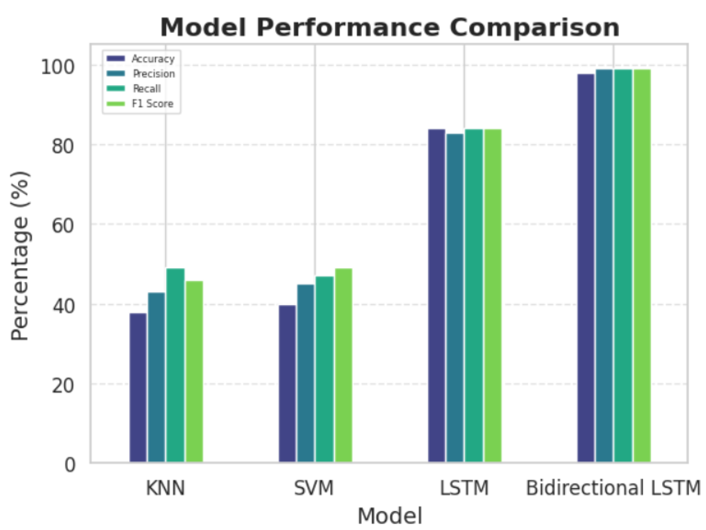
Figure 7.
Accuracy Comparison of different Sliding window lengths
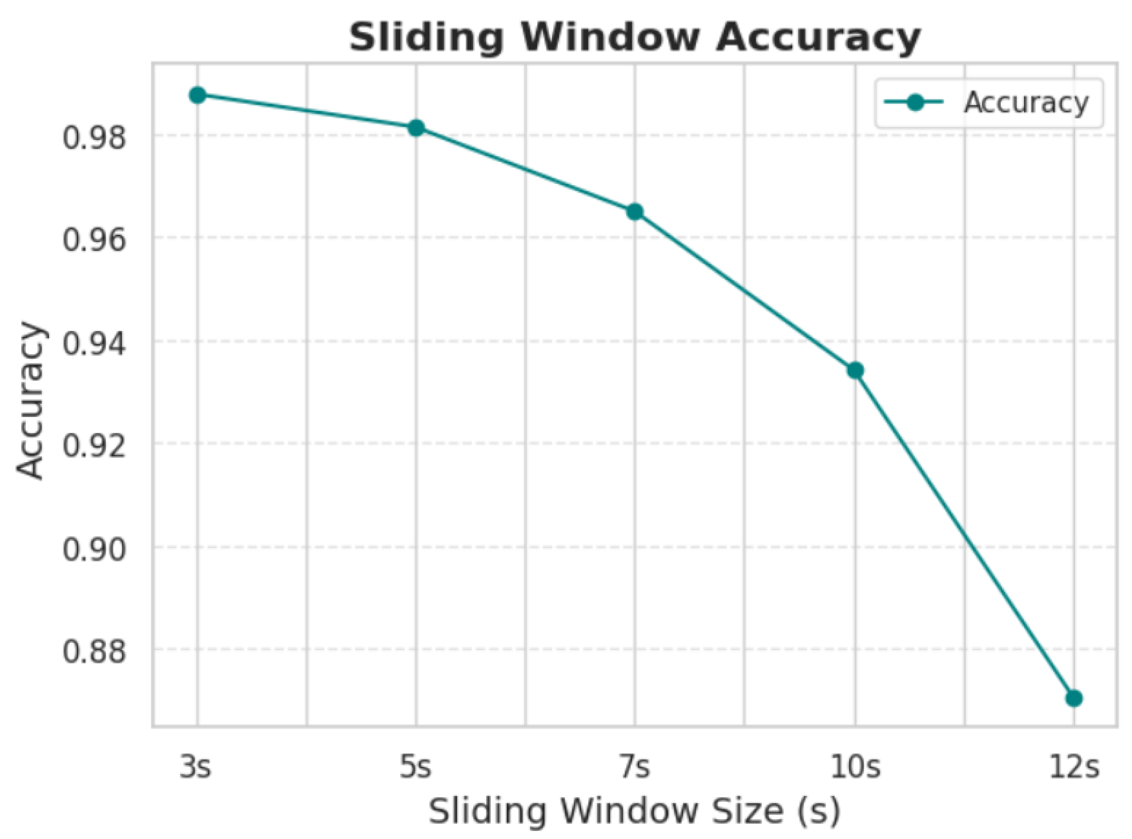
Figure 8.
SHAP summary plot
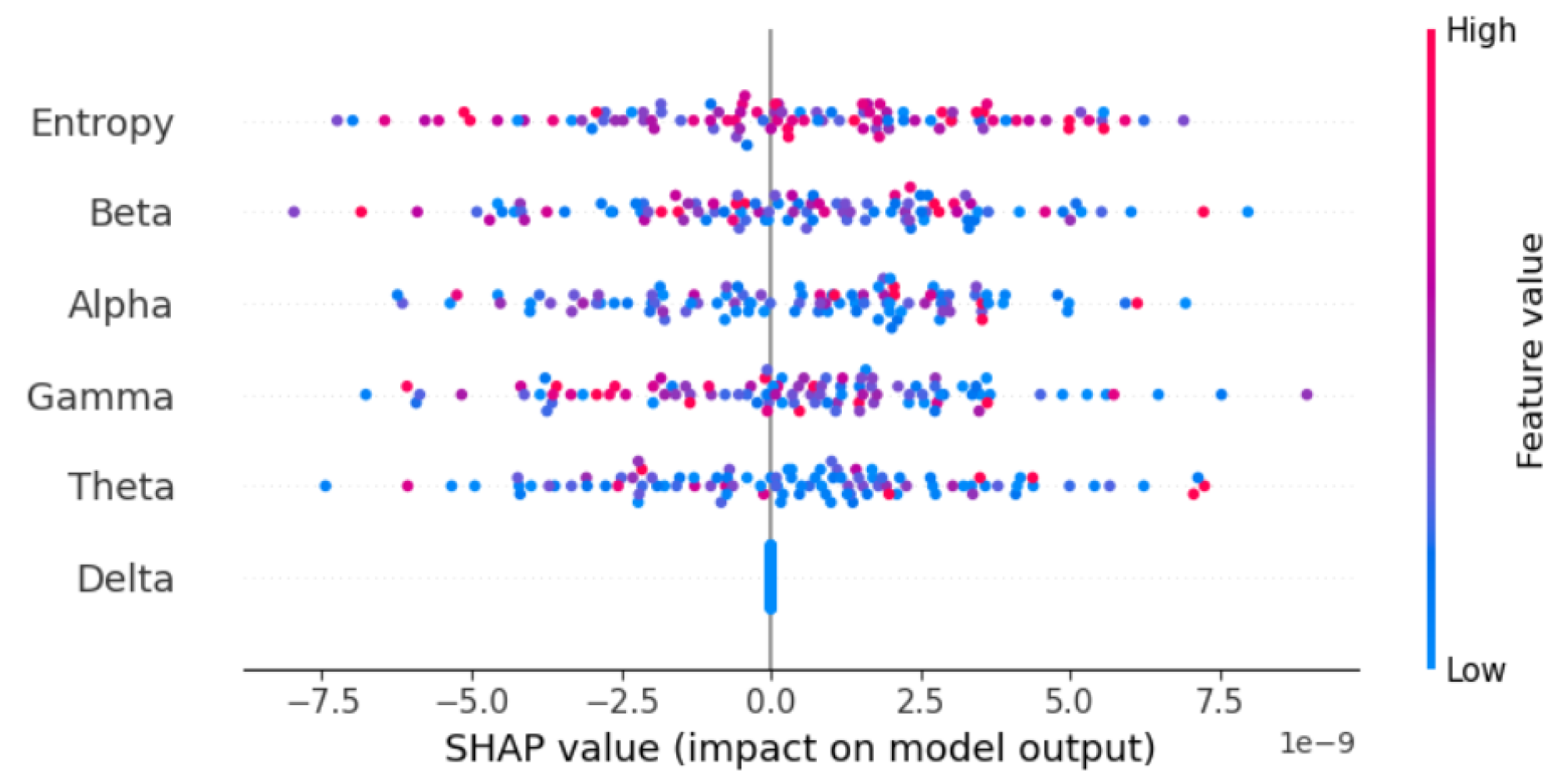
Figure 9.
Features Importance according to SHAP values
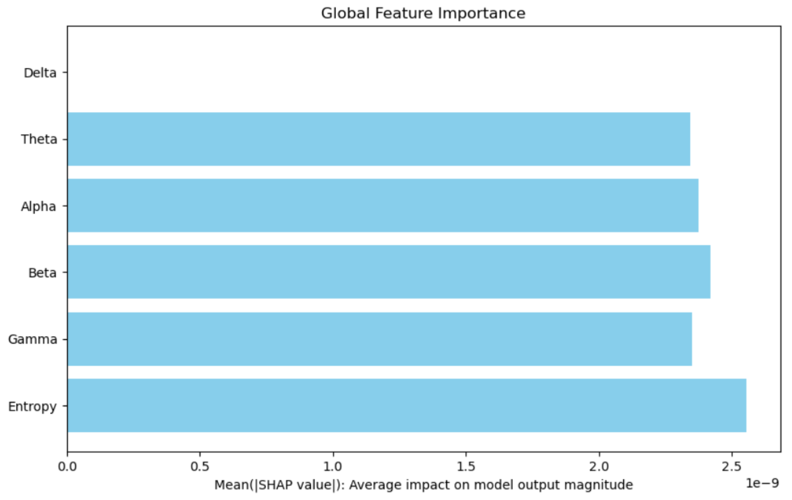

Table 1.
Performance comparison of classification models
| The model | Accurancy | Precision | Recall | F1 Score |
| KNN | 38% | 43% | 49% | 46% |
| SVM | 40% | 45% | 47% | 49% |
| LSTM | 84% | 83% | 84% | 71% |
| Bidrectional LSTM | 98% | 99% | 99% | 99% |
Table 2.
Accuracy comparison for different sliding window lengths in EEG signal processing
| Sliding Window | 3s | 5s | 7s | 10s | 12s |
| Accurancy | 0.987703 | 0.981313 | 0.964953 | 0.934151 | 0.879695 |
Disclaimer/Publisher’s Note: The statements, opinions and data contained in all publications are solely those of the individual author(s) and contributor(s) and not of MDPI and/or the editor(s). MDPI and/or the editor(s) disclaim responsibility for any injury to people or property resulting from any ideas, methods, instructions or products referred to in the content. |
© 2025 by the authors. Licensee MDPI, Basel, Switzerland. This article is an open access article distributed under the terms and conditions of the Creative Commons Attribution (CC BY) license (http://creativecommons.org/licenses/by/4.0/).
Copyright: This open access article is published under a Creative Commons CC BY 4.0 license, which permit the free download, distribution, and reuse, provided that the author and preprint are cited in any reuse.


