Submitted:
03 July 2025
Posted:
07 July 2025
You are already at the latest version
Abstract
Small and medium-sized enterprises (SMEs) are critical contributors to economic growth, innovation and employment. However, they often struggle in securing external financing. This financial gap mainly arises from perceived risks and information asymmetries creating barriers between SMEs and potential investors. To address this issue, our study proposes a machine learning (ML) framework for predicting the investment readiness (IR) of SMEs. All the models involved in this study are trained using data from the survey provided by the European Central Bank's Survey on Access to Finance of Enterprises (SAFE).
In the empirical section of the paper, we train, evaluate and compare the predictive performance of nine (9) machine learning algorithms: Gradient Boosting, Random Forest, Logistic Regression, Support Vector Machines, Naïve Bayes and various ensemble methods. The results highlight the efficiency of ML algorithms in identifying investment-ready SMEs. In particular, the Gradient Boosting algorithm achieves a balanced accuracy of 75.4% and the highest ROC-AUC score at 0.815.
Overall, this study contributes valuable insights to both academics and market participants by demonstrating how machine learning can help in bridging the SME financing gap. It can also offer clear inference to policymakers to design targeted interventions and can provide investors with efficient, data-driven methods for identifying promising SMEs. Ultimately, this research supports the broader goal of enhancing SME access to capital, fostering economic growth through informed policies and decisions, and enhancing the allocation of strategic economic resources.
Keywords:
SMEs
; investment readiness
; machine learning
; SAFE dataset
; equity financing
; economic resilience
; Gradient Boosting
; Random Forest
; Logistic Regression
; SVC
; VIM
Note: The research project is implemented in the framework of H.F.R.I call "Basic Research Financing (Horizontal support of all Sciences)" under the National Recovery and Resilience Plan "Greece 2.0" funded by the European Union – NextGenerationEU (H.F.R.I. Project Number: 16856).

1. Introduction and Literature Review
Small and medium-sized enterprises are defined as enterprises with fewer than 250 employees, having an annual turnover less than 50 million €and/or an annual balance sheet total less than = 43 million € (Commission of the European Communities, 2003/361/EC). They play a crucial role in economic growth, employment, and innovation. They account for approximately 90% of all businesses globally, providing over half of the total employment and significantly contributing to GDP across various economies (World Bank, 2023). Despite their crucial role, SMEs frequently struggle to secure adequate external financing, limiting their potential for growth and innovation. This issue is particularly acute in emerging markets, where about 40% of formal SMEs report unmet financing needs (World Bank, 2023). The financing gap faced by SMEs is often due to information asymmetries and the perception of higher risk, causing lenders and investors to be cautious when considering investments in smaller firms. As traditional financial institutions generally rely on established credit histories and collateral—requirements, many SMEs cannot meet—these enterprises often resort to internal funding or informal finance sources (Mason & Harrison, 2001, Douglas & Shepherd, 2002).
Investment readiness—the ability of an SME to attract and secure external funding—has emerged as an important concept to bridge the financing gap. A firm that is "investment ready" typically demonstrates a sound and viable business model, credible financial reporting, clear growth potential, and an effective management team capable of communicating these strengths to potential investors (Douglas & Shepherd, 2002). Yet, previous research consistently finds a mismatch between SMEs’ self-assessments of readiness and investors' evaluations, resulting in many firms being overlooked despite having solid business foundations (Fellnhofer, 2015).
Traditional approaches for evaluating SME investment readiness, such as financial ratios, scoring systems and qualitative assessments, have significant limitations. These methods often overlook complex, non-linear relationships within the data and rely heavily on past financial performance, potentially disregarding other vital aspects like managerial capability or innovation (Mullainathan & Spiess, 2017; Dumitrescu et al., 2021). In response, machine learning (ML) techniques have begun to gain prominence due to their ability to analyze large, multidimensional datasets and identify complex, predictive patterns that traditional econometric methods might miss (Dumitrescu et al., 2021).
Given these challenges and opportunities, this paper applies advanced ML methods to assess the investment readiness of SMEs, using the European Central Bank's (ECB) Survey on Access to Finance of Enterprises (SAFE) dataset. This large-scale, cross-national dataset offers extensive qualitative and quantitative information on SMEs' financial conditions, their market positions, innovation activities, and management capabilities—factors critical for assessing investment readiness.
Investment Readiness and SME Financing
Investment readiness is a multidimensional concept reflecting an enterprise’s capacity to understand and satisfy investor expectations as captured through business planning, financial transparency, growth prospects and managerial competence. Mason and Harrison (2001) emphasized that simply increasing the availability of venture capital without ensuring SMEs are investment-ready is insufficient to address funding gaps. Many entrepreneurs are often perceived by investors as "not ready" due to weak financial documentation, unrealistic growth expectations or an aversion to equity dilution. Douglas and Shepherd (2002), similarly, found discrepancies in perceptions of investment readiness between entrepreneurs and investors highlighting the importance of clear communication and alignment of expectations to improve SMEs' chances of securing financing.
Investment readiness programs have been developed globally to bridge these gaps by providing targeted training and support to SMEs, improving their business plans, enhance financial transparency and overall investability (Cusolito, Dautovic, & McKenzie, 2021). However, despite their importance, such programs typically yield only modest improvements and may not fully resolve systemic issues such as informational asymmetries and entrenched investor biases (Owen et al., 2023).
Recent studies have shown that machine learning (ML) methods significantly outperform traditional econometric models in forecasting complex financial market behavior. ML models, unlike traditional approaches, can handle vast and multidimensional datasets, uncovering and capturing complex and intricate relationships and interactions between variables (Du & Rada, 2010; Khan et al., 2023). For instance, Dumitrescu et al. (2021) demonstrated how hybrid ML-econometric models significantly improve credit scoring by combining predictive accuracy with interpretability.
Despite the promising potential of ML approaches, existing research on their application specifically to SME investment readiness remains limited. Most studies focus on broader financial forecasting contexts or specific applications such as credit risk or stock market prediction, leaving a notable research gap regarding the application of ML in predicting SME investment readiness.
Additionally, while investment readiness programs have been implemented globally to support SMEs, their effectiveness in addressing structural financing gaps remains minimal, suggesting the need for more sophisticated, data-driven assessment tools (Cusolito, Dautovic, & McKenzie, 2021; Owen et al., 2023).
From a venture capital perspective, enhancing screening efficiency to identify promising SMEs remains a challenge. The potential for ML to significantly streamline this screening process, reducing biases and enhancing deal-flow quality, has not yet been thoroughly examined in academic research (Zana & Barnard, 2019). From a venture capital perspective, investment readiness screening is essential due to the high-risk nature of early-stage financing. Venture capitalists often reject many SMEs at early screening stages due to insufficient preparedness in terms of management capabilities, realistic financial projections, and business viability (Mason & Kwok, 2010; Zana & Barnard, 2019). While human judgment remains essential, integrating machine learning that is independent of related human biases and misjudgments into the venture screening process could significantly streamline identification efforts, reducing biases and expanding the search for investment ready SMEs beyond personal networks (Zana & Barnard, 2019).
Our research directly addresses these gaps by empirically evaluating multiple advanced ML algorithms, i.e., Gradient Boosting, Logistic Regression, Random Forest, and ensemble methods, using a comprehensive and robust dataset provided by the European Central Bank’s Survey on Access to Finance of Enterprises (SAFE). By explicitly linking managerial competencies, innovation, and openness to equity financing to SME investment readiness through ML techniques, this study contributes both methodologically and substantively to the entrepreneurial finance literature. It does not only advance predictive accuracy, but also offers actionable insights for SMEs, investors, and policymakers, ultimately aiming to enhance resource allocation efficiency and support broader economic growth and innovation.
2. Data and Research Methodology
2.1. Data Collection and Pre-Processing
The dataset was collected from the European Central Bank Data Portal and contains anonymous qualitative responses from micro, small, medium and large companies across Europe. The dataset provides insights into the financing conditions faced by these companies.
The dataset was thoroughly cleaned by removing duplicates, non-SME entries, sparse features, and variables closely tied to the target to ensure data relevance and prevent leakage and contamination. After cleaning, the final dataset contained 10937 SME entries (rows) each described by 59 variables (columns). The dataset is heavily imbalanced with 12% of entries belonging to class 1 (investment ready class) and the remaining 88% to class 0 (non-investment ready class). Categorical variables were converted to numerical format using dummy encoding, creating binary columns to represent each category.
The binary target variable takes the value of 1 when the SME is investment ready, and 0 in the opposite case. We define an SME as investment ready (IR) when it is:
- Innovative: these are the firms that have reported new developments, such as introducing a new product or service to the market, implementing a new production process or method, adopting new management practices, or exploring new ways of selling goods or services.
- Fast growing: these are the cases where the annual turnover increases by more than 20%.
- Open to equity financing: whether it reported equity as either a relevant funding source or one used in the past six months.
2.2. Machine Learning Algorithms
Machine learning is the branch of Artificial Intelligence which allows a machine -an algorithm- to learn from data and improve its performance without being explicitly programmed. ML algorithms analyze historical data to identify simple or complex patterns or to make predictions. As Norvig and Russel state, 2020, “the process where the computer observes some data, builds a model based on the data and uses it as a hypothesis about the world and as a software that can solve problems” is called Machine Learning. Supervised learning is described as the type of machine learning where the algorithm learns and produces a model (function) from labeled training data. The goal is for the system to generalize from these examples, meaning that it can efficiently produce the correct output to new and unseen inputs (Russel, Norvig, 2020).
Logistic Regression
Logistic Regression is a statistical method of classification. It is an algorithm that models the probability of a discrete outcome. While it shares similarities with linear regression in terms of using a linear combination of input features, the key distinction is that Logistic Regression applies a non-linear logit (log-odds) transformation to model the probability of the outcome. Logistic Regression is considered relatively interpretable among classification methods because the sign of each coefficient indicates whether a predictor positively or negatively influences the outcome’s log-odds. However, the exact effect of a unit change in an input on the predicted probability is not directly intuitive due to the non-linear (logistic) transformation. In other words, while one can relate coefficient values to odds ratios translating those into absolute probability changes requires additional calculation. The algorithm can also incorporate regularization techniques such as L1 (Lasso), L2 (Ridge) or ElasticNet regularization norms, which help prevent overfitting and improve generalization by penalizing the excessively large coefficients of the model (Cox, 1958).
K-Nearest Neighbors
The K-Nearest Neighbors algorithm is a non-parametric, instance-based learning machine learning method. Rather than learning an explicit model from the training data, K-NN makes predictions by directly referencing the stored training examples. For a given instance, the algorithm identifies the k closest data points (neighbors) in the feature space, typically using a distance metric such as Euclidean distance. The predicted class for the instance is the ruling class among these neighbors. Choosing a small value of k can lead to overfitting, as the model becomes sensitive to noise in the training data, while a large value of k may result in underfitting by oversmoothing class boundaries (Cover, Hart 1967).
Random Forest
Random Forest classifier is an ensemble learning algorithm that builds multiple decision trees and combines their outputs. Each tree in the forest is trained on a random subset of the data, selected through bootstrap sampling (sampling with replacement), and at each split within a tree, a random subset of features is considered for determining the best split. This combination of data and feature randomness helps reduce overfitting and enhances the model’s generalization ability. For classification tasks, the final prediction is determined by majority voting. Random Forests are well-suited for high-dimensional datasets, are robust to noise, and generally maintain a degree of interpretability through feature importance measures (Breiman, 2001).
Support Vector Machines
Support Vector Machines are a powerful class of supervised machine learning algorithms used for classification and regression tasks. SVMs aim is to locate the (optimal) hyperplane that maximizes the distance between the hyperplane and the closest data points of different classes, known as support vectors. When data is not linearly separable, Support Vector Machines utilize the kernel trick, which maps the input features into a higher dimensional space where a linear separation between the classes is possible. In our experiments we used the radial basis function kernel and the linear kernel. Regularization in SVMs helps balance the trade-off between fitting the training data well and maintaining generalization to new data (Cortes, Vapnik, 1995).
Naïve Bayes
Naïve Bayes is a probabilistic classifier based on Bayes' Theorem, used to classify data by estimating the probability that a given instance belongs to a particular class. It is termed “naïve” because it assumes that the features (or attributes) are conditionally independent of each other given the class label. In Naïve Bayes classification, the algorithm estimates the prior probabilities for each class by calculating the frequency of appearance of each class in the dataset. It, then, computes the likelihood of observing that feature value given the class. For a new unknown instance, the classifier computes the posterior probability for each possible class. Posterior probability is the probability that an instance belongs to a class C given the features X. The class with the highest posterior probability is selected as the predicted class (Manning, Raghavan, Schuetze 2008).
AdaBoost
Adaptive Boosting (AdaBoost) is an ensemble machine learning algorithm that combines multiple weak classifiers to create a strong classifier. It works by sequentially training a series of simple models, in our case shallow decision trees, on repeatedly modified versions of the data. In each new model the algorithm focuses on the instances misclassified by the previous ones. AdaBoost assigns higher weights to misclassified samples, compelling subsequent models to focus on these hard-to-classify cases. The final prediction is made by aggregating the outputs of all weak classifiers through a weighted majority vote, where classifiers with better accuracy have greater influence(Freund, Schapire, 1995).
Easy Ensemble
The Easy Ensemble classifier was introduced by Liu, Wu et al. (2009) to address imbalanced classification problems by leveraging ensemble learning. It consists of multiple AdaBoost classifiers, each trained on distinct, balanced bootstrap samples. To achieve balance, the method applies random under-sampling in the majority class ensuring that both classes will have equal representation in the sub-sample. Each iteration of the algorithm involves training an AdaBoost model using a different sub-sample. This process is repeated several times, generating multiple classifiers. The final prediction is produced through a voting mechanism of all models. By repeatedly resampling the majority class and boosting weak learners, Easy Ensemble effectively improves classification performance on imbalanced datasets while maintaining the strengths of boosting techniques.
Balanced Bagging Classifier
Balanced Bagging classifier is an ensemble method designed to address the class imbalance in classification tasks. It is a variation of the traditional Bootstrap Aggregating (Bagging) algorithm, where multiple models are trained in parallel, and their predictions are combined to make the final decision. The key difference is that Balanced Bagging classifier also handles the class imbalance. The classifier creates multiple subsets of the original data by randomly sampling data points with replacement. The subsets are balanced before the training of each classifier. The balance of the class labels is done by random under-sampling on majority class to match the size of the minority class. Then each classifier is trained on the balanced subsets. The final prediction is being made by utilizing the majority voting concept on classification tasks (Breiman, 1996).
Gradient Boosting Trees
Gradient boosting classifiers are additive models, where the prediction for a given input is made by combining the outputs of several weak learners, which in our problem are Decision Trees. The Gradient Boosting model is built iteratively in a greedy fashion, where each new tree is trained to correct the errors (residuals) made by the previous trees. Initially, the model starts with a constant value, the mean of the target values, to minimize the loss. During each iteration, the model computes the residuals - the differences between the observed and predicted values and fits a Decision Tree to these residuals. The tree is adjusted to minimize the loss function, and the model is updated by adding the contribution of the new tree. This process is repeated for a set number of trees (weak learners), with each tree improving the model by correcting the errors of previous ones.
Cross Validation
Before applying any machine learning algorithm, we first split the dataset into a) the train set that is used to locate the best hyperparameters and identify the optimal models, and b) the validation set, that is never used in the previous process (training) and used to evaluate the out-of-sample performance of the trained models.
A critical aspect of machine learning model development is managing the trade-off between overfitting and underfitting. Underfitting occurs when a model is unable to capture the underlying structure of the data, often due to excessive simplicity or insufficient training, and is typically reflected in poor performance across both the training and validation datasets. Overfitting occurs when a model becomes too complex relative to the amount of training data, leading it to memorize noise and idiosyncrasies within the specific training set. As a result, while training accuracy may be high, the performance on any new and unseen data, like the validation dataset, degrades significantly. In either case, the model fails to generalize beyond the training distribution. To mitigate overfitting, cross-validation techniques are employed to evaluate the model’s performance across multiple data partitions, providing an estimate of its predictive accuracy on unseen data.
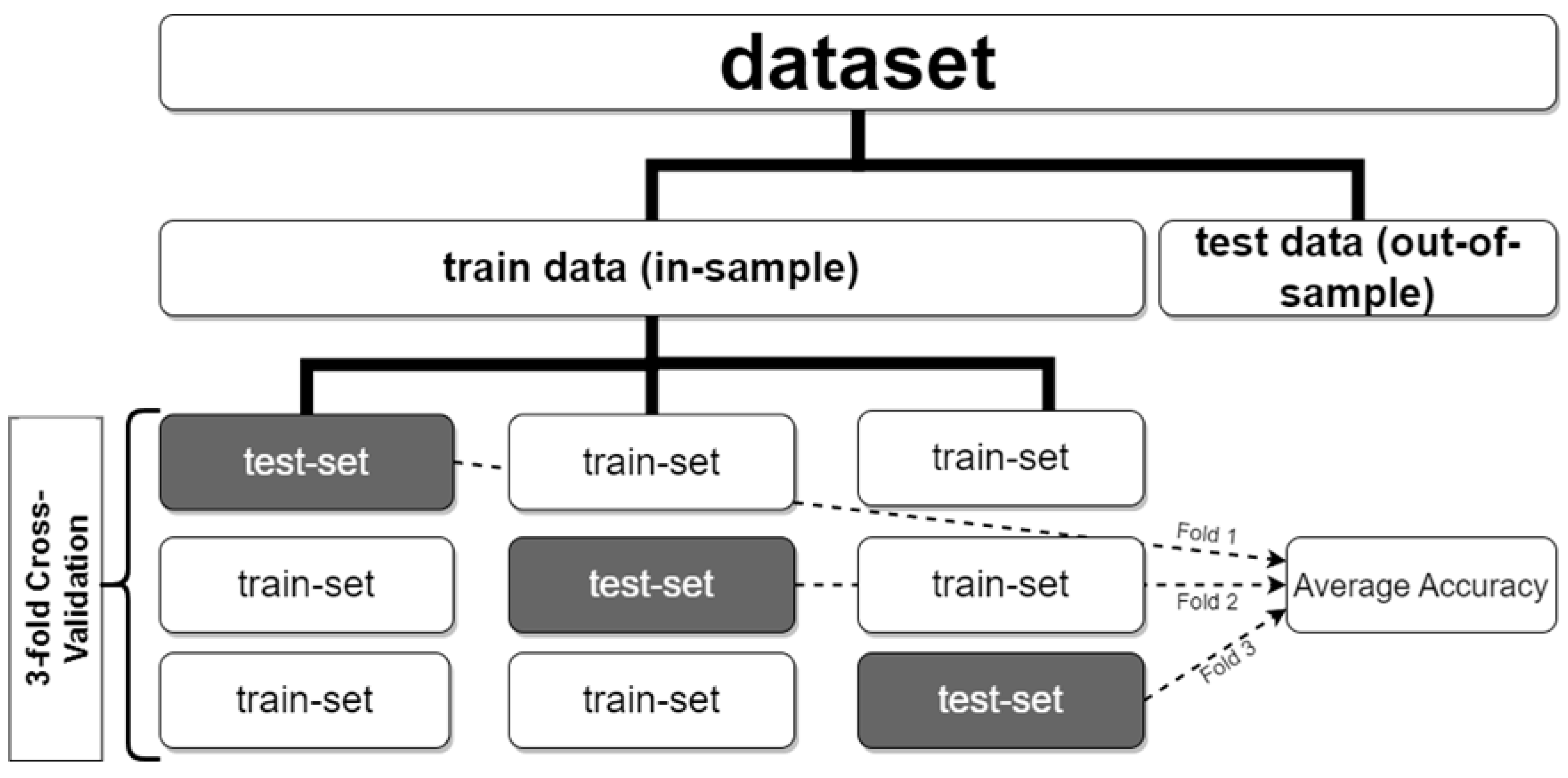
Thus, to start the training process, we employed a cross-validation technique, and the training dataset is partitioned into 5 equal-sized folds and the training is repeated iteratively; in each iteration, 4 folds are used for training the model, while the remaining fold is used for testing. This process is repeated 5 times, with each fold serving as the test set once. For each unique set of hyperparameters, a new model is trained, and the corresponding test scores are averaged and used to identify the optimal model. Given the class imbalance in the dataset, where the minority class (class 1), comprises only 12% of the observations, we employed a stratified 5-fold cross-validation technique, rather than simple random sampling for the folds, to ensure that all folds are consistent. This ensures that each fold maintains roughly the same class distribution as the original dataset, thereby providing stable and representative validation results.
Figure 1.
A graphical representation of a 3-fold cross validation process. A graphical representation of a 3-fold cross validation process. For every set of hyperparameters test, each fold serves as a test sample, while the remaining folds are used to train the model. The average performance for each set of parameters over the k test folds was used to identify the best model. (Gogas et al., 2019).
Model Selection
Nine classification algorithms were used in this paper. The hyperparameter tuning process was conducted using the grid search technique, a systematic approach that exhaustively explores a predefined subset of the hyperparameter space. Grid search iteratively evaluates combinations of hyperparameters by fitting models to the training data and assessing their performance using the stratified 5-fold cross-validation scheme. The optimal hyperparameters for each algorithm were chosen based on the highest average performance in cross-validation on the test sets. The classification algorithms applied in the experimental analysis are the following:
- Logistic Regression
- K-Nearest Neighbor
- Random Forest
- Support Vector Machines with RBF and linear kernel
- Naïve Bayes Classifier
- AdaBoost
- Easy Ensemble
- Balanced Bagging Classifier
- Gradient Boosting Trees
Data Imbalance
To address the issue of the imbalanced dependent variable, the models were trained using balanced class weights. This approach involves assigning higher weights to the underrepresented class (class 1 – Is Investment Ready) and lower weights to overrepresented class (class 0 – Is Not Investment Ready) during the training process. By doing this, the model is penalized more for misclassifying the minority class observations, encouraging it to pay more attention to the less frequent instances.
2.3. Forecasting Performance Metrics
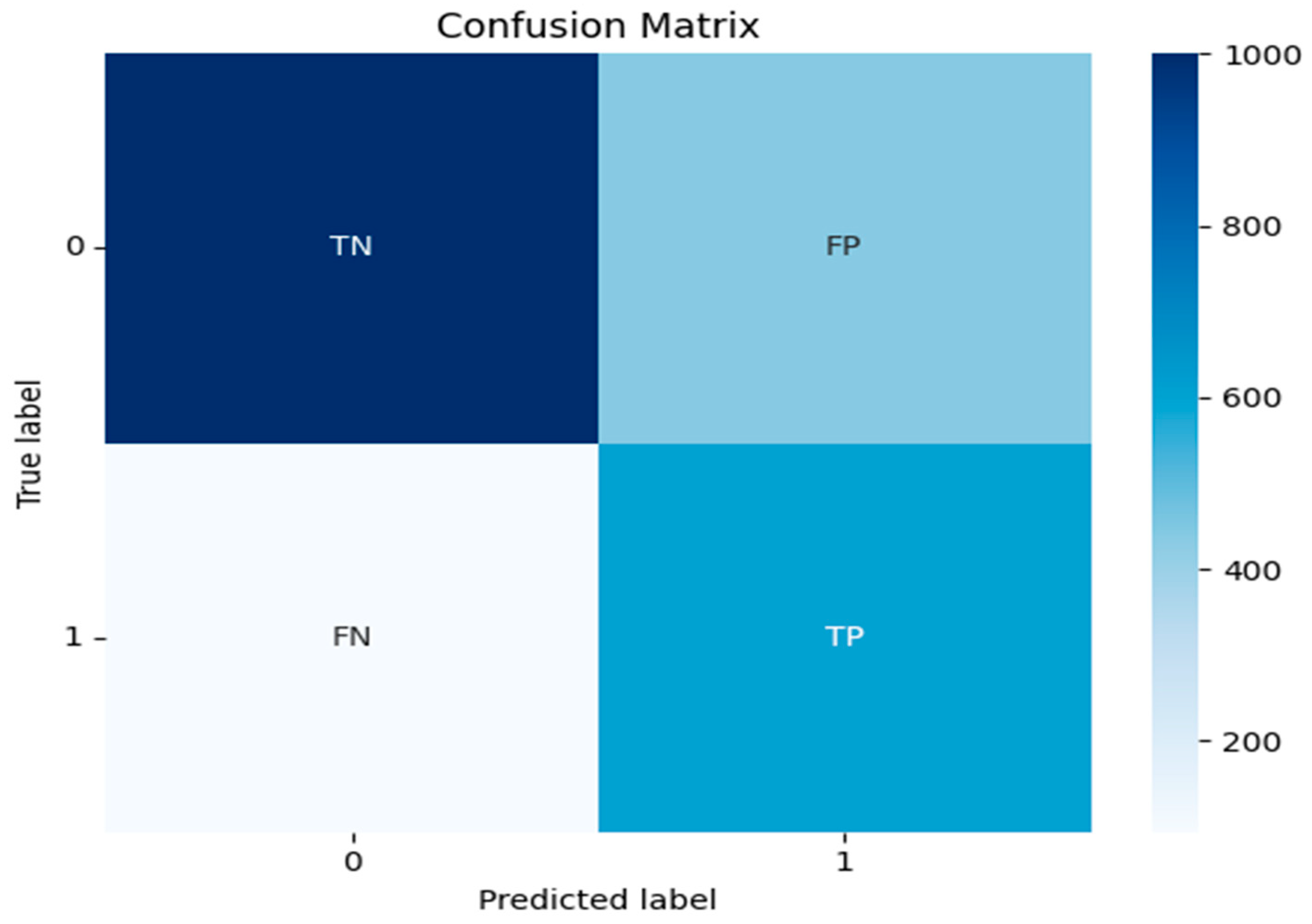
In a binary classification problem, normally, a confusion matrix is created to visually summarize the models’ performance. The confusion matrix consists of four values as below:
- True Positives (TP): The number of instances that the model correctly predicts the positive class (in our case the SME to be predicted as investment-ready, class 1).
- True Negatives (TN): The number of instances that the model correctly predicts the negative class (in our case the SME to be predicted as non-investment-ready, class 0).
- False Positives (FP): The number of instances that the model incorrectly predicts the positive class when the actual class is negative.
- False Negatives (FN): The number of instances that the model incorrectly predicts the negative class when the actual is positive.
Figure 2.
Confusion Matrix.
From these values above, various metrics are being defined and have been used to evaluate our models as below:
Precision
Measures the reliability of positive predictions for each class:
Class 0 (not investment-ready):
It counts the proportion of companies forecasted as "not investment-ready" that are truly non-investment-ready. High precision indicates high confidence in negative predictions.
Class 1 (investment ready):
In this case, the precision measures the proportion of companies predicted as "investment-ready" that are truly investment-ready. High precision reduces false positives (e.g., mislabeling non-investment-ready companies as investment-ready).
Recall (Sensitivity/Specificity)
Measures the models’ ability to identify all relevant instances of a class:
Class 0 Recall (Specificity):
Recall of class 0 counts the ability of the model to correctly identify non-investment-ready companies.
Class 1 Recall (Sensitivity):
Recall of class 1 counts the ability of the model to correctly identify investment-ready companies.
F1-Score
Balances precision and recall using their harmonic mean. A high F1-Score indicates strong performance in both precision and recall for a class. It is critical for evaluating the investment-ready (minority) class, where both false positives (costly misallocations) and false negatives (missed opportunities) are consequential.
or alternatively,
Balanced Accuracy
While accuracy is the standard metric for evaluating classification models on balanced datasets, it becomes less informative in the presence of class imbalance, as in our case. In such data, the balanced accuracy measure is preferred. Defined as the average recall (sensitivity) across all classes, balanced accuracy offers a more reliable assessment of model performance by accounting for sensitivity in each class explicitly. Balanced accuracy can also be interpreted as class-wise accuracy weighted by class prevalence in the dataset (Brodersen, Ong et al., 2010).
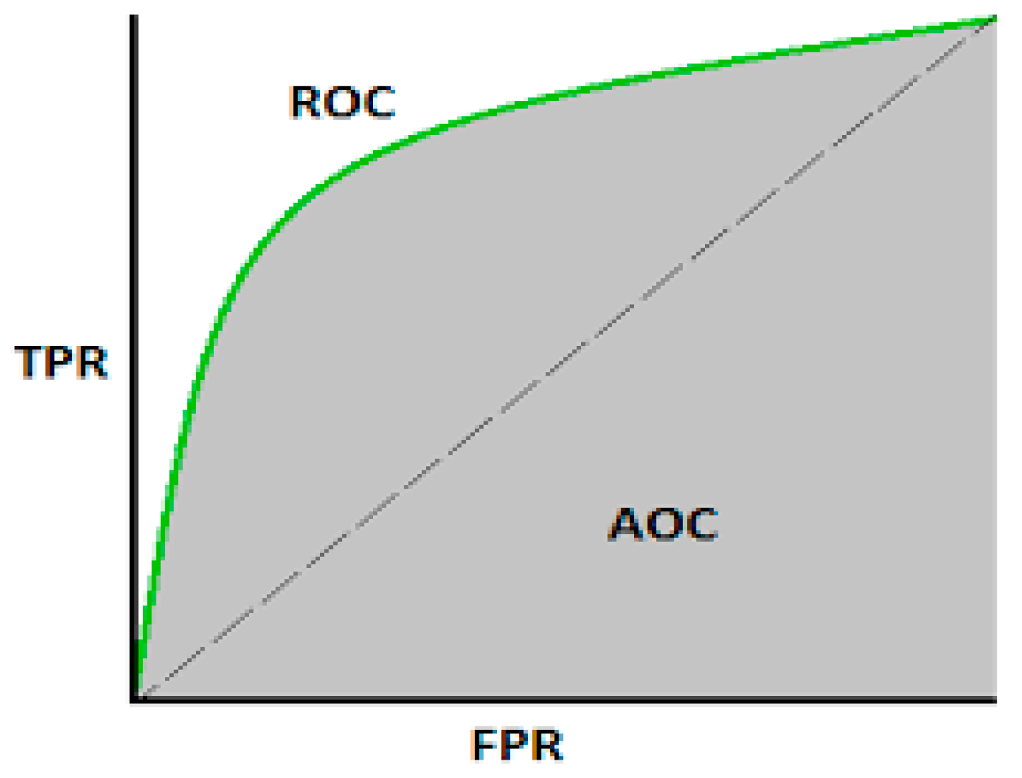
Receiver Operating Characteristic Area Under Curve (ROC-AUC)
The ROC-AUC quantifies the model’s ability to discriminate between classes. The ROC curve plots the true positive rate (sensitivity) against the false positive rate (1-specificity) at various threshold settings, while the area under curve (AUC) ranges from 0.5 (no discriminative power, equivalent to random guessing) to 1 (perfect discrimination).
Figure 3.
ROC AUC Curve.
All the above metrics matter. High precision in Class 0 ensures non-investment ready companies are correctly filtered out. High recall in Class 1 ensures investment ready companies are not overlooked, while Class 1 precision avoids costly false positives. F1-score and balanced accuracy provide a single metric to balance these trade-offs, especially vital for an imbalanced dataset.
2.4. Variable Importance Measure (VIM)
In tree-based models, the VIM is used to assess and rank the contribution of each variable to the model's predictive performance. During the construction of a decision tree, the algorithm selects variables at each split based on how well they improve the model’s ability to distinguish between classes. This is typically done by minimizing a metric known as impurity (e.g. Gini impurity or entropy). Variables that consistently result in greater reductions of impurity across the tree are considered more important. The VIM reflects this by aggregating the impurity reductions attributed to each variable over the entire tree (or forest, in ensemble models like Random Forest), helping to identify which features have the most influence on the model's decisions.
3. Empirical Results
Given the significant class imbalance in our dataset (88% non-investment-ready vs 12% investment-ready), the simple accuracy is not an adequate forecasting metric. A naïve classifier that classifies as "non-investment-ready" all instances of the dataset would achieve an 88% accuracy while failing entirely to identify investment-ready firms. Balanced accuracy addresses this limitation as we described above. By averaging the recall rates for both classes, balanced accuracy gives equal importance on investment-ready and non-investment-ready companies, regardless of their proportions in the dataset. Therefore, we use the balanced accuracy score to rank the models’ overall performance and identify the best model.
The balanced accuracy scores of our models range from 55.2% to 75.4%. Gradient Boosting created the best model, with a balanced accuracy of 75.4%, followed by the Logistic Regression with 75%. In Figure 3, Figure 4 and Figure 5, we present the results for all models and various performance metrics. We can see that the Gradient Boosting model outperforms all other models for both class-wide metrics, namely Balanced Accuracy and ROC-AUC. When looking at class 1 metrics, it achieved some of the best performance, only slightly falling behind in terms of Recall and Precision, where the models that excelled in those metrics were the Logistic Regression and the Random Forest respectively. However, Gradient Boosting having the Best F1 score for class 1 indicates that it offers the best trade-off between precision and recall, making it the most well-rounded model for discovering promising SMEs.
Figure 4.
Balanced Accuracy and ROC-AUC.
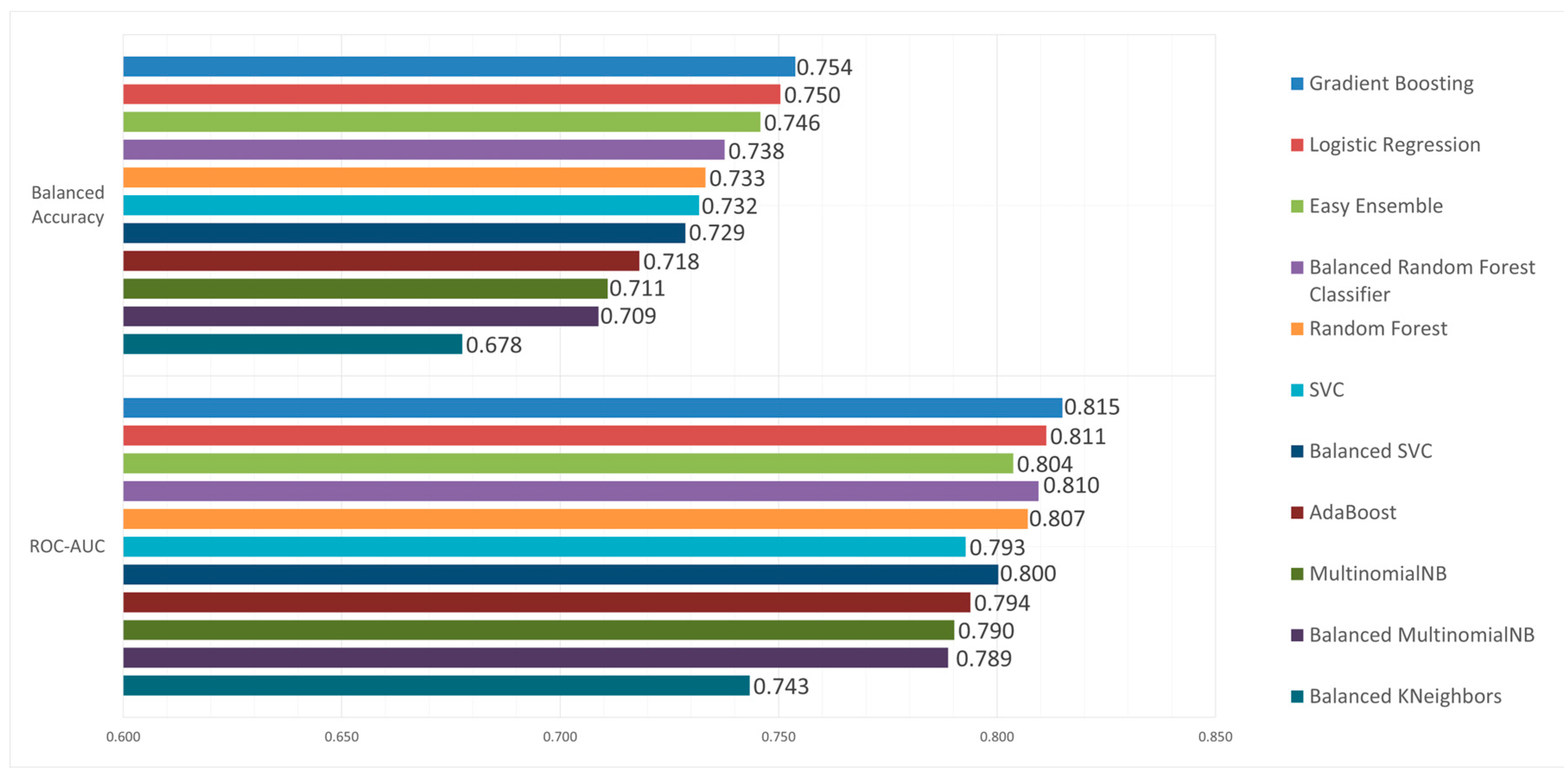
Figure 5.
Class 0 Metrics.
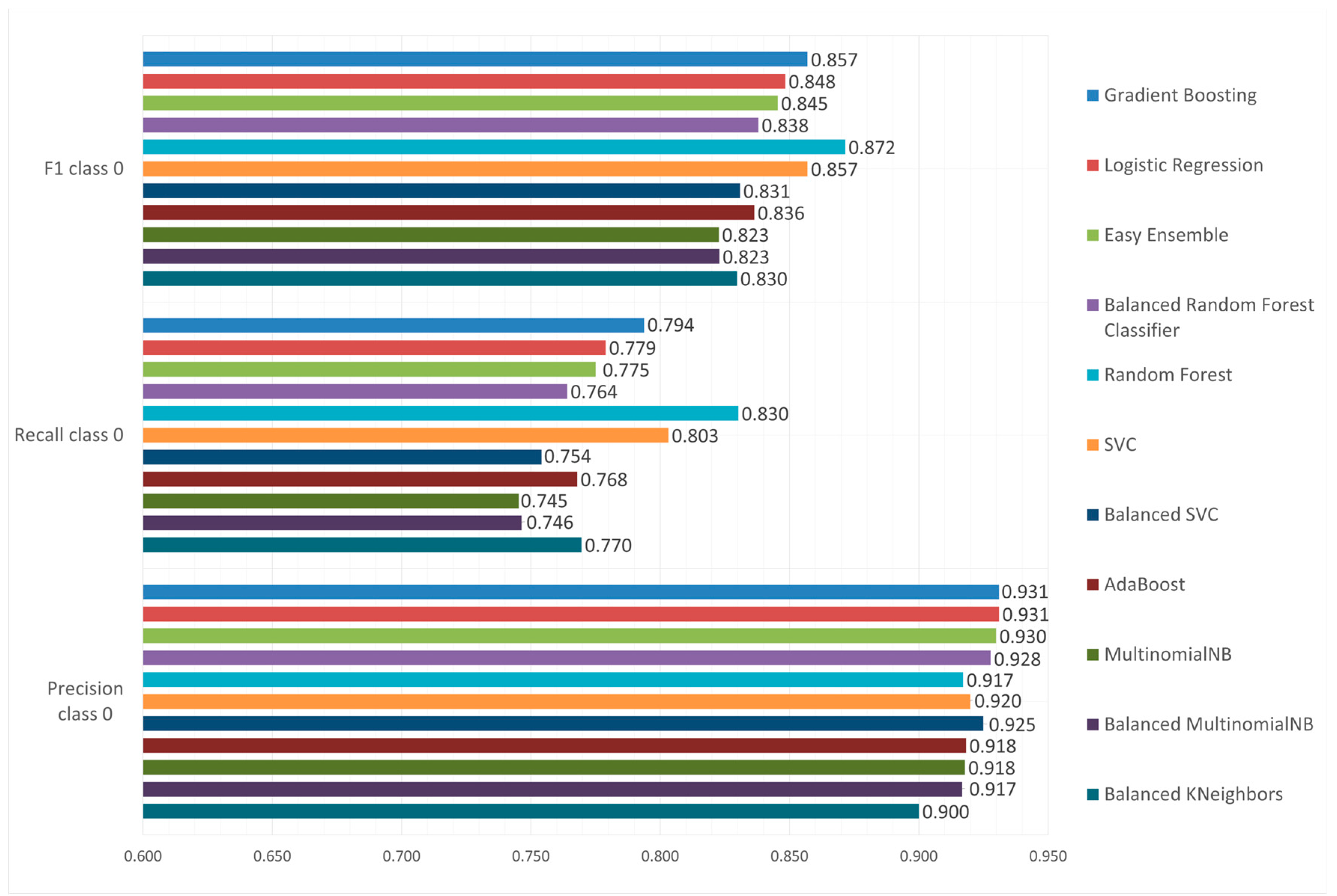
Figure 6.
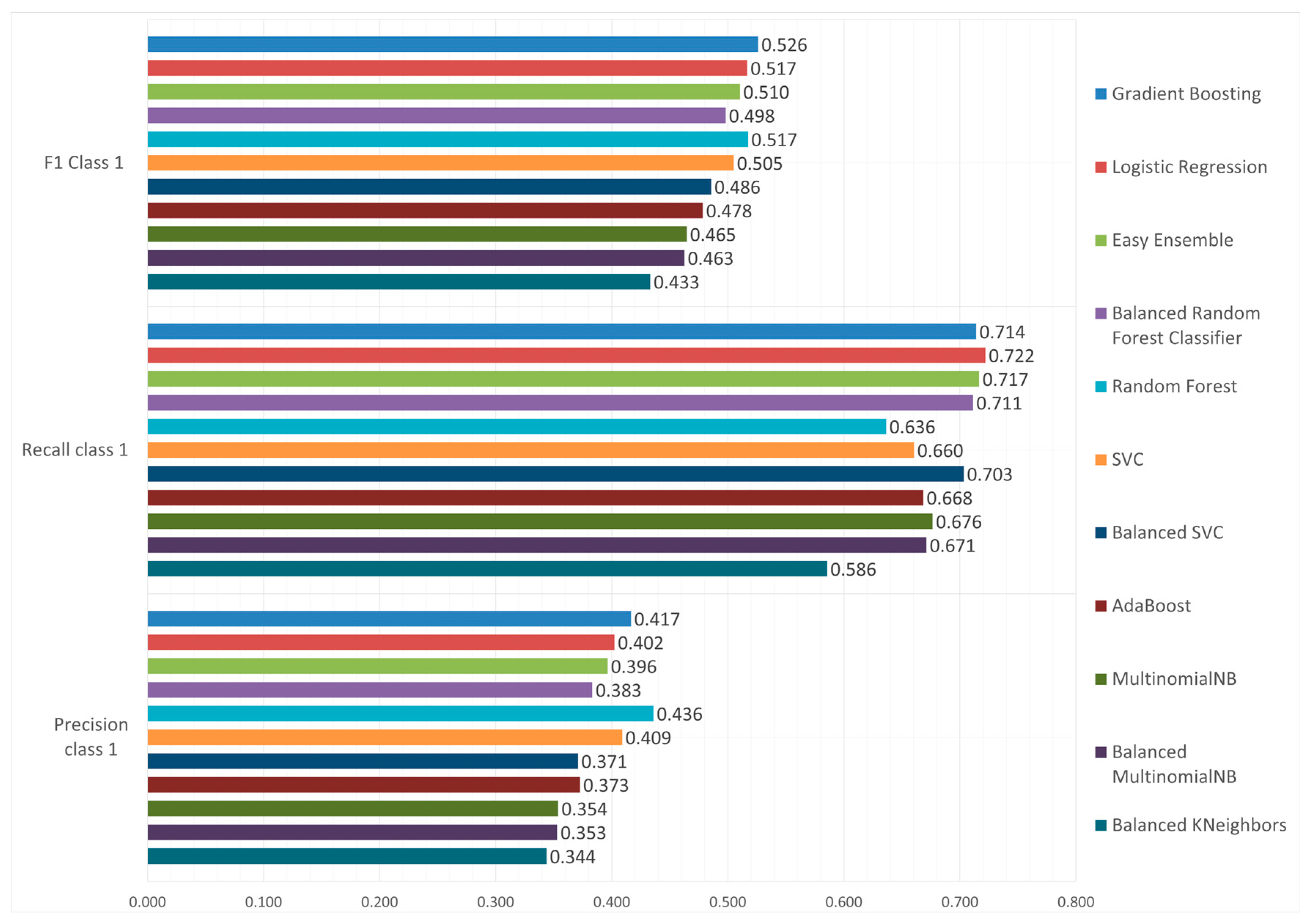
Class 1 Metrics.
Moreover, in Figure 7 below, we present the ROC Curve for the Gradient Boosting model.
Despite its algorithmic simplicity, the Logistic Regression has demonstrated a remarkable performance, particularly in class 1 recall reaching 0.722; the highest of all models. The Logistic Regression had a balanced accuracy of 0.750 and an ROC-AUC score of 0.811, which are second only to Gradient Boosting. Easy ensemble shows consistent performance across metrics. While not leading in any metric, with a balanced accuracy of 0.746, a precision of 0.396 and a recall of 0.717, its consistent performance suggests robustness in its capabilities. With an F1-score of 0.510 and ROC-AUC of 0.804, it performs only slightly worse than the two leading models. Finally, the Balanced Random Forest had the third highest ROC-AUC score of 0.810, only marginally worse than Logistic Regression and had a competitive recall rate of 0.711. Nonetheless, it has the lowest balanced accuracy (0.738) and precision (0.383) among the top models.
Considering Precision, Recall, and F1, Gradient Boosting appears to outperform most of the competition for class 0, exhibiting some of the top values across all evaluation metrics. The model achieved the best overall precision of 0.931, with the second highest overall Recall score of 0.794 and the second highest F1-score of 0.857 only falling behind the Random Forest, which had a recall score of 0.830 and an F1 score of 0.872.
Precision remains consistent across all models with a limited variability (Precision variance of models is 0.031). The same is not true for Recall (Recall variance of models is 0.128). All models achieve exceptional Class 0 precision (>90%) with Gradient Boosting offering the optimal performance.
Overall, Gradient Boosting is the optimal model for predicting SME investment readiness and is the recommended model in terms of creating a balanced predictive strategy. There are however models that excel at specific metrics, like the Logistic Regression in terms of class 1 Recall or Random Forest in terms of class 0 Recall. Classifying the majority class proved to be an easy task for all of the models, having achieved very high levels of both precision and F1-scores. This indicates that the algorithms were effective at filtering out non-investment-ready firms. On the other hand, predicting the minority class proved to be a challenge. This is made evident by the overall lower F1-scores all of the models, which peaked at 0.526 and low precision levels. This highlights the challenge in avoiding false positives.
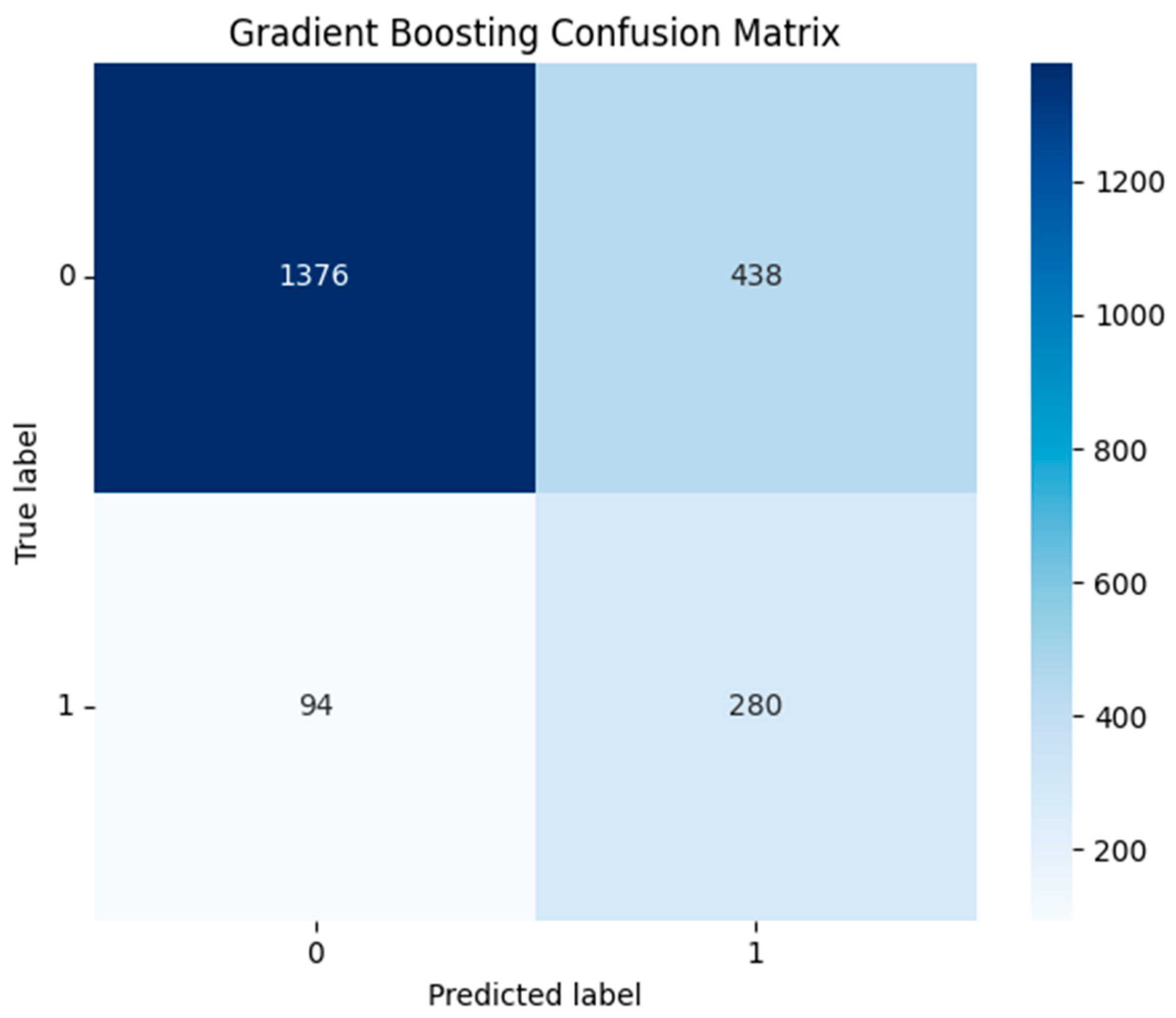
In Figure 8 and Figure 9 below, we present the confusion matrix and the normalized confusion matrix respectively for the best model, the Gradient Boosting. It achieved:
- 267 TP predictions (investment-ready) out of 374, or 71.3%.
- 1440 TN predictions (not-investment-ready) out of 1814 or 79.3%.
- 374 FP predictions (predicted as investment-ready but are not) or 20.6%
- 107 FN predictions (predicted as not-investment-ready but are not) or 28.6%.
The confusion matrices for the rest of the models are included in the appendix.
Applying the Variable Importance Measure (VIM) technique to our best model, the Gradient Boosting, the 10 most important variables and their ranking is presented in Figure 10. The variable importance plot illustrates the relative contribution or each input feature to the model’s classification performance with higher values indicating greater influence on the model’s predictions. Out of the 10 most important variables ranked according to the VIM, the first six are comparatively the most prominent.
- The most important predictor appears to be the firm’s “confidence in negotiations with equity investors or venture capital firms”. High levels of negotiation confidence likely reflect firm preparation, understanding of investor expectations, and stronger business fundamentals, all of which are critical traits for attracting external investment.
- The second most important predictor is “financing growth”, which indicates that the firms that are actively seeking and managing financial growth, tend to be investment ready. This highlights the importance of proactive financial planning and scaling strategies as indicators of a firm’s investment potential.
- “Factors in the future of financing of the firm” is ranked third in top predictors. This variable points to the importance of future financial planning. Investors may favor firms that not only demonstrate current performance but also show foresight in securing future financing.
- “External financing factors” including market conditions or access to funding channels is also an essential feature that influences the model’s decision-making process. Firms capable of navigating external factors-influences may be more successful in attracting external investors.
- “Autonomous organization type”, relating to the structure of the organization plays the fourth more important role on predicting an investment ready SME. Autonomous firms might be more agile and able to innovate and thus they draw investors’ interest.
- “Willingness of investors to invest in the enterprise”, relating to the investors’ sentiment towards the firm.
These six variables summarize the importance of both a) internal factors such as confidence, growth, future outlook, and the firm’s autonomy and flexibility and b) external factors such as market conditions, availability of financing and the overall sentiment of the investors’ towards investing in a firm.
Cost function
Another way to assess the forecasting efficiency of the selected algorithms and identify the best model is by calculating and including in the evaluation process the misclassification cost. This is done by using a cost function in the selection of the optimal model. The cost function that we used is defined as:
Total Misclassification Cost (TMC) = CFP FP + CFN FN
where CFP is the cost of a false positive forecast, CFN is the cost of a false negative forecast, FP is the total number of false positive cases, and FN the total number of false negative cases. In our case, we set CFP =1 and CFN = 5. The use of such a weighted cost is part of the cost-sensitive evaluation methodology studied in classification problems with unequal errors (Peykani et al, 2025). Table 1 presents for each one of the five best models the FN, FP and the resulting TMC for each model. The use of such a weighted cost is part of the cost-sensitive evaluation methodology studied in classification problems with unequal errors (Peykani et al, 2025).
The Gradient Boosting model exhibits the lowest TMC (908) and making it the best model even under the cost sensitive criterion. Thus, it is the best forecasting model even when we impose the Cost Function as a model selection criterion. The Logistic Regression produces a slightly higher TMC cost (914) indicating comparable cost performance. These results confirm that accounting for misclassification costs refines our evaluation: while Gradient Boosting was already strong by balanced accuracy, it also minimizes the economic cost of errors under our cost assumptions.
Under the cost-optimized threshold (0.452), the confusion matrix for the Gradient Boosting model is:
Figure 11.
Gradient Boosting Confusion Matrix normalized.
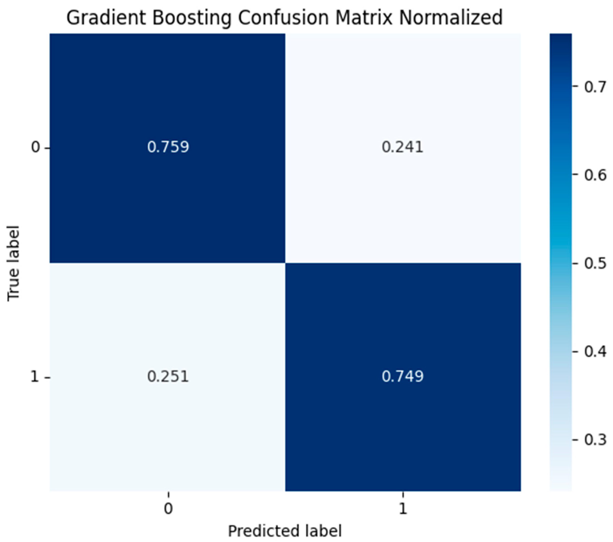
Figure 12.
Gradient Boosting Confusion Matrix .
4. Conclusion
The primary goal of this research was to apply advanced machine learning (ML) techniques to predict SME investment readiness, utilizing the large data set collected by the Survey on Access to Finance of Enterprises (SAFE) conducted semiannually by the European Central Bank. After training and evaluating multiple ML algorithms that included: Gradient Boosting, Logistic Regression, Random Forest, and various ensemble methods, the Gradient Boosting model demonstrated the highest predictive performance, with a balanced accuracy of 75.4% and an ROC-AUC score of 0.815. The Logistic Regression was notably close in performance, indicating that simpler, interpretable models can also effectively predict investment readiness, providing practical benefits in scenarios requiring rapid deployment or interpretability.
Although explicit feature selection was not implemented in this study, our findings highlight several important factors influencing investment readiness. These factors include managerial confidence, innovation activities, openness to equity financing, and investor engagement. Clearly identifying these factors helps SMEs strategically prioritize improvements, thereby enhancing their likelihood of securing external financing.
From an academic perspective this research adds valuable insights to the entrepreneurial finance literature by demonstrating the practical effectiveness of machine learning techniques in financial decision-making. However, the close performance between Gradient Boosting and Logistic Regression underscores the continued relevance of traditional econometric models, particularly in situations where interpretability and prompt results are crucial.
The economic implications are considerable. Independent investors, relevant governmental agencies, and financial institutions can leverage these predictive models to better assess SMEs, minimizing costly misinvestments (Type I errors). Consequently, such models have the potential to optimize the allocation of the already scarce private and government financial resources. Policymakers can utilize these insights to tailor more effective support programs for SMEs addressing their specific financing needs. Ultimately, adopting these predictive approaches promises more efficient capital markets, enabling SMEs to contribute more effectively to economic growth and job creation.
An additional insight from the cost evaluation is that the selection of the best model can shift significantly once the economic implications of misclassifications are accounted for. When both costs (false positive and false negative) are adequately measured and assigned to the optimization of the predictive models, a model with higher balanced accuracy is not necessarily the one with the lowest overall cost. When the two costs are asymmetric as it was assumed in this paper and the cost of a false negative is greater than the cost of a false positive, the precision as a model selection metric would be inferior to the recall (sensitivity). This is because the latter focuses on maximizing the identification of true positives that is the same as minimizing false negatives. This analysis confirms that cost-sensitive evaluation complements and adjusts the overall findings, providing more practical and economically sensitive guidance for model selection in real-world scenarios.
Appendix A

Table A1.
Confusion Matrix Metrics for all models.
| Model | TN | FP | FN | TP |
| Gradient Boosting | 1440 | 374 | 107 | 267 |
| Logistic Regression | 1413 | 401 | 104 | 270 |
| Easy Ensemble Classifier | 1406 | 408 | 106 | 268 |
| Balanced Random Forest Classifier | 1386 | 428 | 108 | 266 |
| Random Forest | 1506 | 308 | 136 | 238 |
| SVC | 1457 | 357 | 127 | 247 |
| Balanced SVC | 1368 | 446 | 111 | 263 |
| AdaBoost | 1393 | 421 | 124 | 250 |
| MultinomialNB | 1352 | 462 | 121 | 253 |
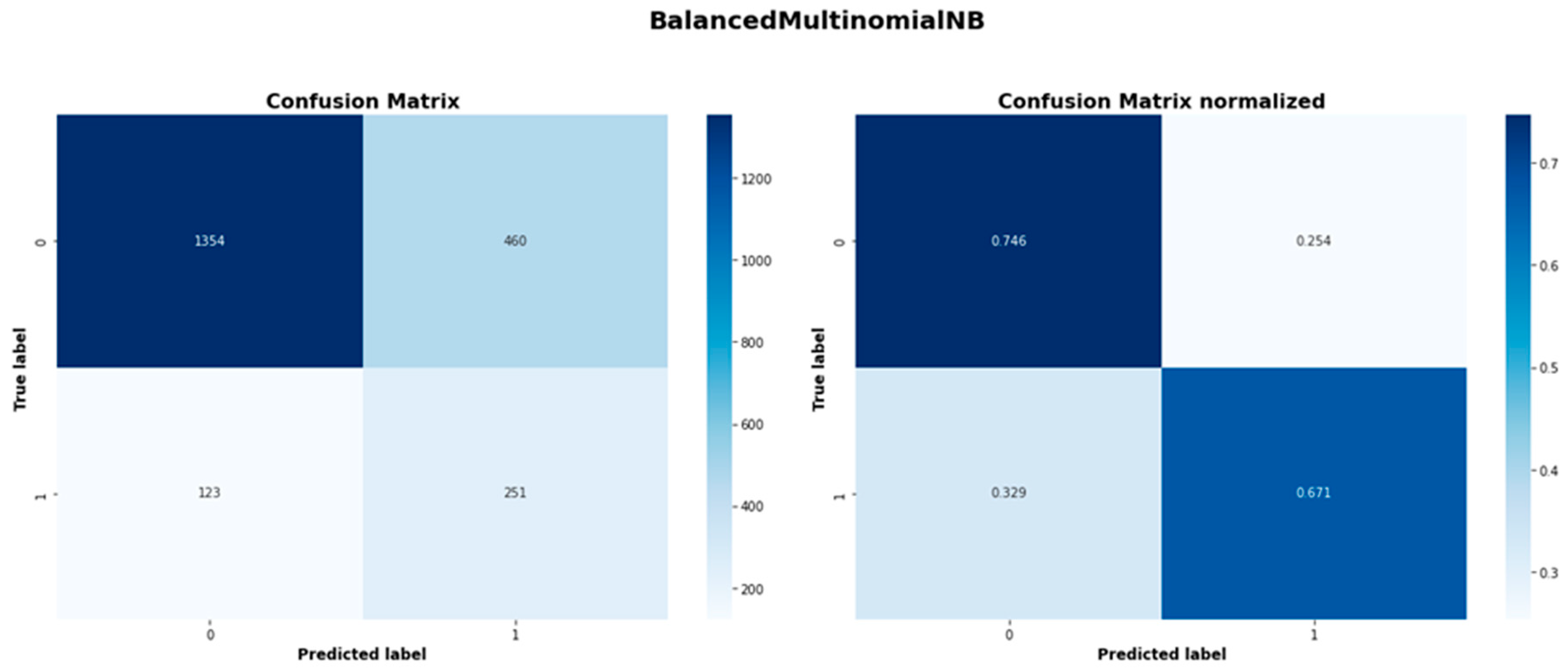
| Balanced MultinomialNB | 1354 | 460 | 123 | 251 |
| Balanced KNeighbors | 1396 | 418 | 155 | 219 |
| KNeighbors | 1745 | 69 | 321 | 53 |
Table A2.
Balanced Accuracy and ROC-AUC score for all models.
| Model | Balanced Accuracy | ROC-AUC |
| Gradient Boosting | 0.754 | 0.815 |
| Logistic Regression | 0.750 | 0.811 |
| Easy Ensemble Classifier | 0.746 | 0.804 |
| Balanced Random Forest Classifier | 0.738 | 0.810 |
| Random Forest | 0.733 | 0.807 |
| SVC | 0.732 | 0.793 |
| Balanced SVC | 0.729 | 0.800 |
| AdaBoost | 0.718 | 0.794 |
| MultinomialNB | 0.711 | 0.790 |
| Balanced MultinomialNB | 0.709 | 0.789 |
| Balanced KNeighbors | 0.678 | 0.743 |
| KNeighbors | 0.552 | 0.640 |
Table A3.
Precision, Recall and F1 score for all models.
| Model |
Precision class 0 |
Recall class 0 |
F1 class 0 |
Precision class 1 |
Recall class 1 |
F1 Class 1 |
| Gradient Boosting | 0.931 | 0.794 | 0.857 | 0.417 | 0.714 | 0.526 |
| Logistic Regression | 0.931 | 0.779 | 0.848 | 0.402 | 0.722 | 0.517 |
| Easy Ensemble Classifier | 0.930 | 0.775 | 0.845 | 0.396 | 0.717 | 0.510 |
| Balanced Random Forest Classifier | 0.928 | 0.764 | 0.838 | 0.383 | 0.711 | 0.498 |
| Random Forest | 0.917 | 0.830 | 0.872 | 0.436 | 0.636 | 0.517 |
| SVC | 0.920 | 0.803 | 0.858 | 0.409 | 0.660 | 0.505 |
| Balanced SVC | 0.925 | 0.754 | 0.831 | 0.371 | 0.703 | 0.486 |
| AdaBoost | 0.918 | 0.768 | 0.836 | 0.373 | 0.668 | 0.478 |
| MultinomialNB | 0.918 | 0.745 | 0.823 | 0.354 | 0.676 | 0.465 |
| Balanced MultinomialNB | 0.917 | 0.746 | 0.823 | 0.353 | 0.671 | 0.463 |
| Balanced KNeighbors | 0.900 | 0.770 | 0.830 | 0.344 | 0.586 | 0.433 |
| KNeighbors | 0.845 | 0.962 | 0.899 | 0.434 | 0.142 | 0.214 |
Figure A1.
Gradient Boosting confusion matrices.
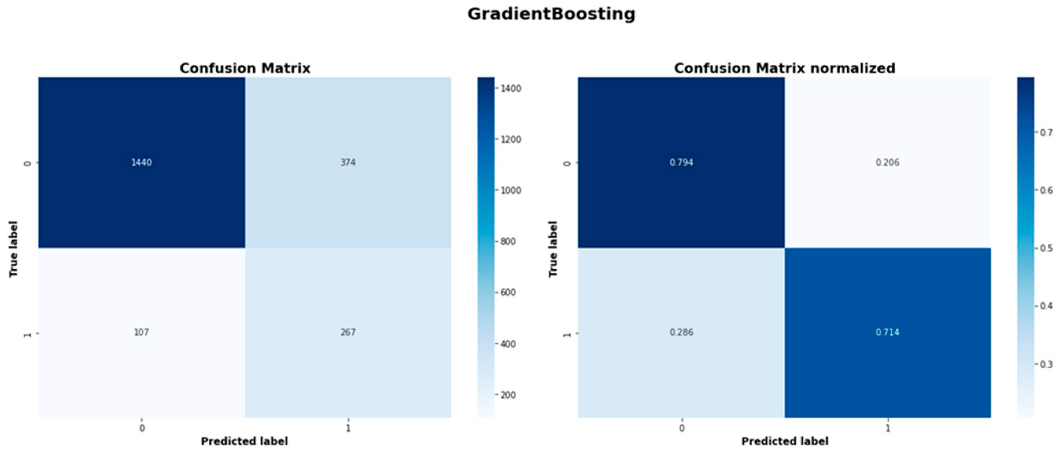
Figure A2.
Logistic Regression model confusion matrices.
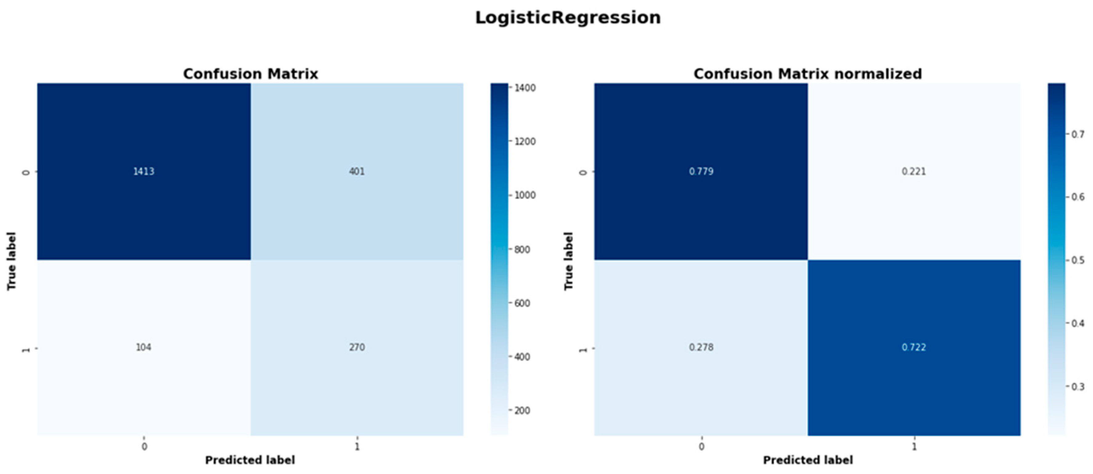
Figure A3.
Easy Ensemble Classifier model confusion matrices.

Figure A4.
Balanced Random Forest model confusion matrices.
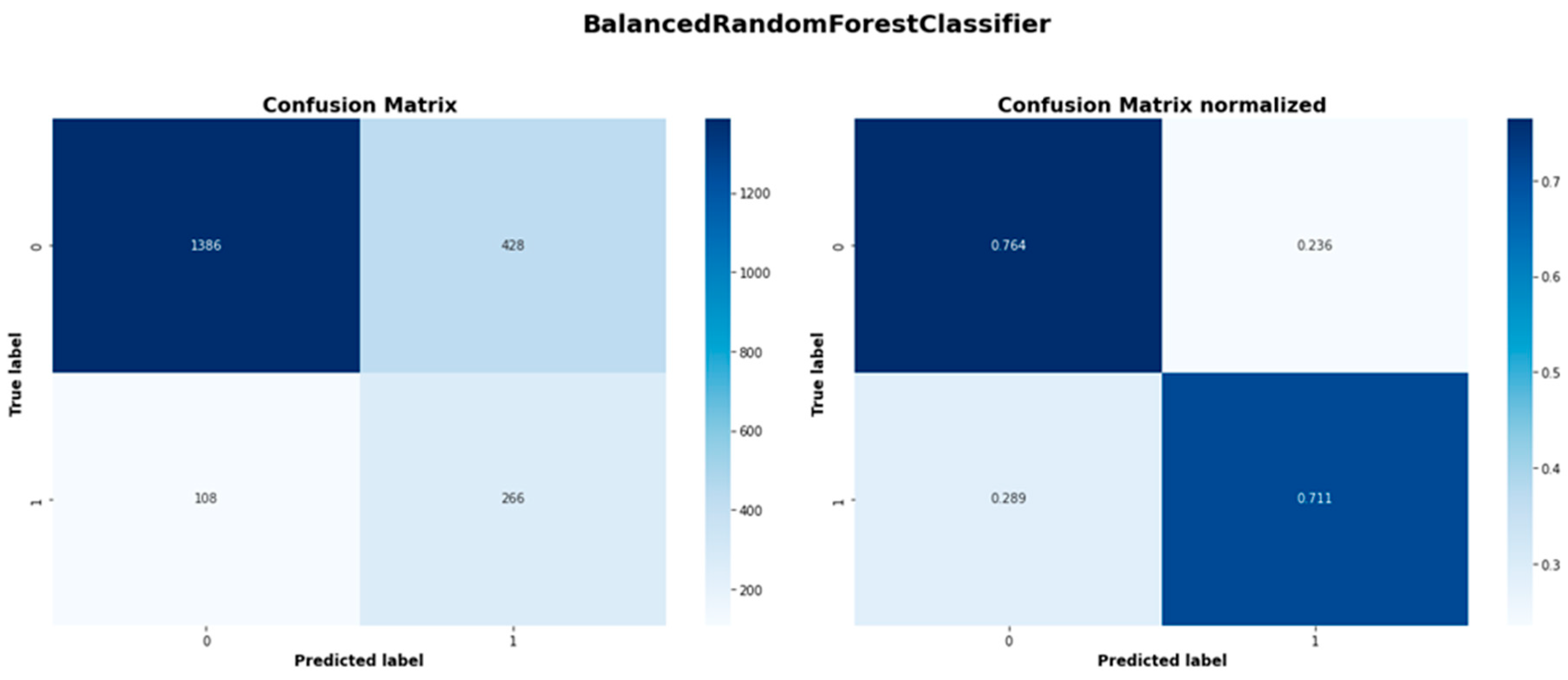
Figure A5.
Random Forest model confusion matrices.
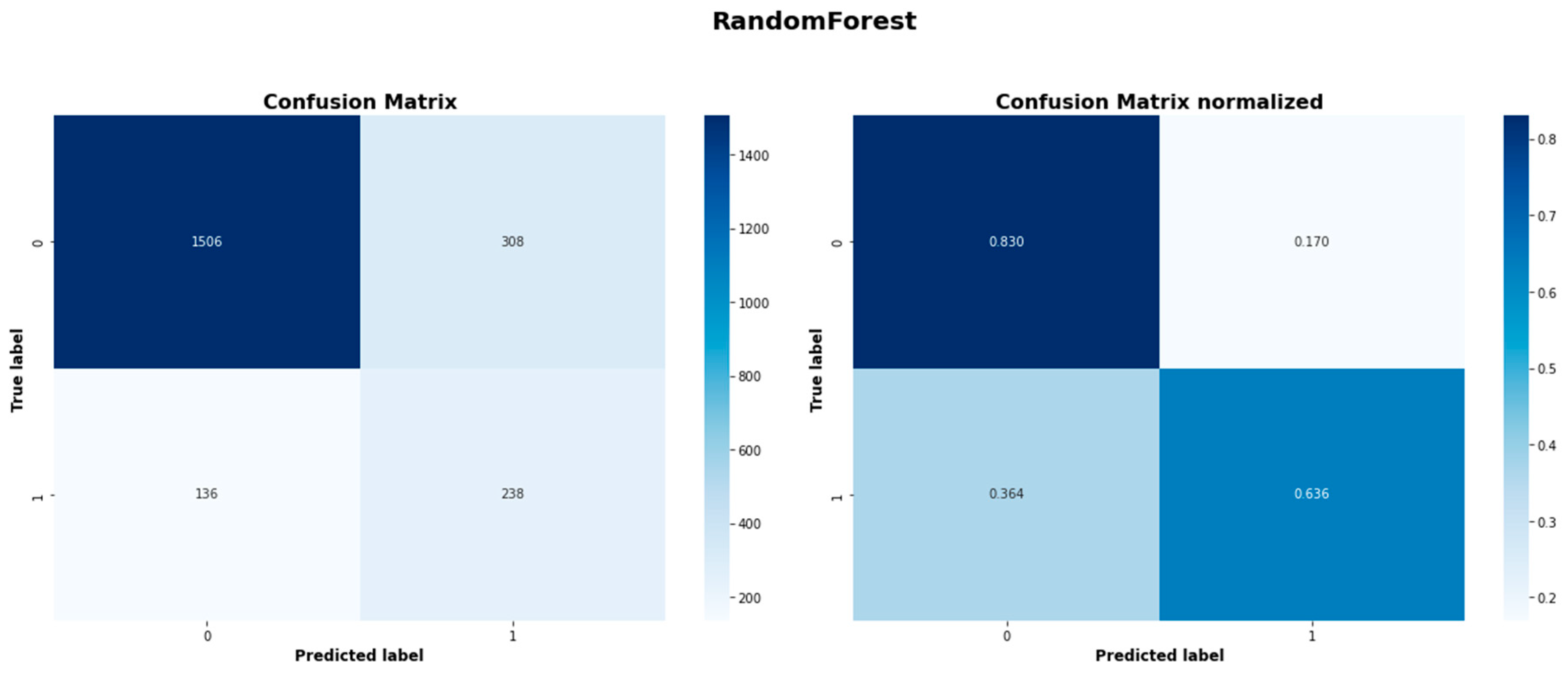
Figure A6.
SVC model confusion matrices.
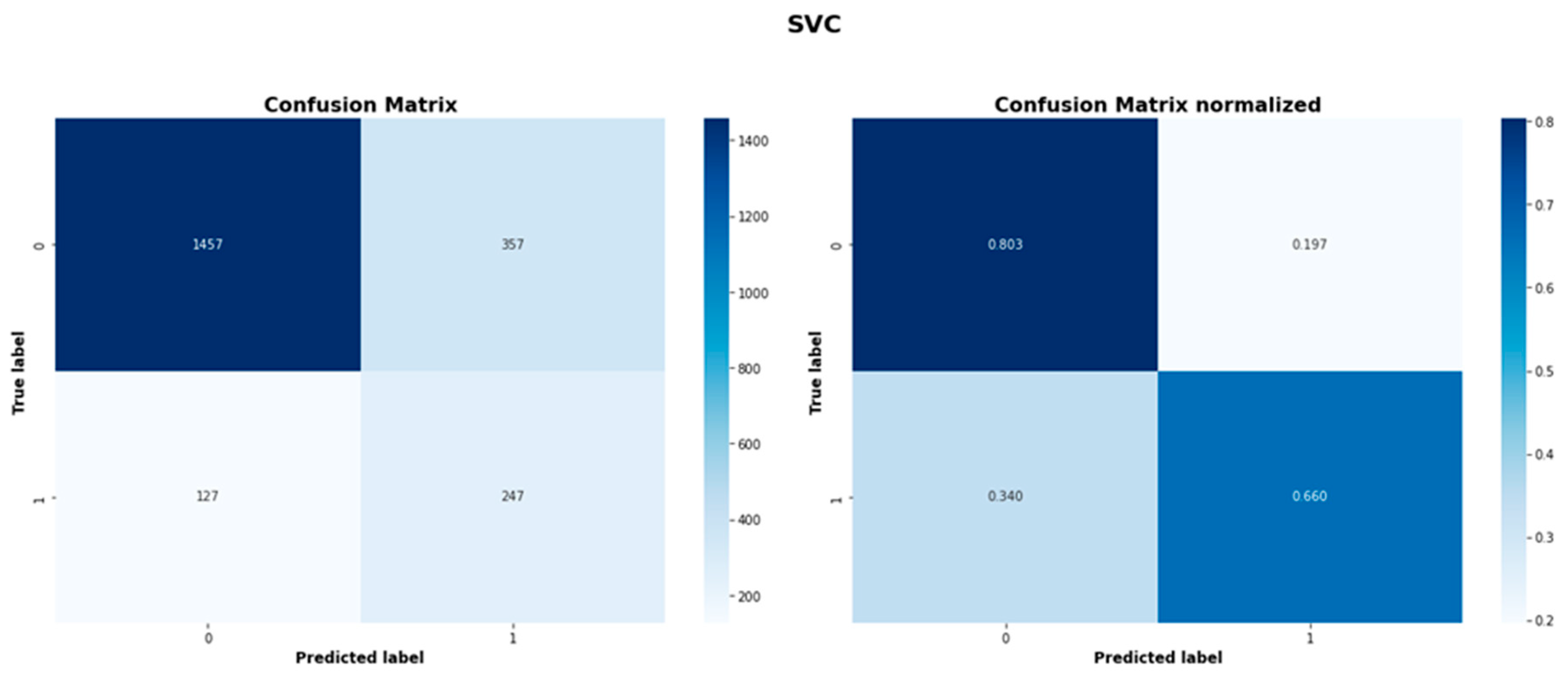
Figure A7.
Balanced Bagging SVC model confusion matrices.

Figure A8.
Adaboost model confusion matrices.
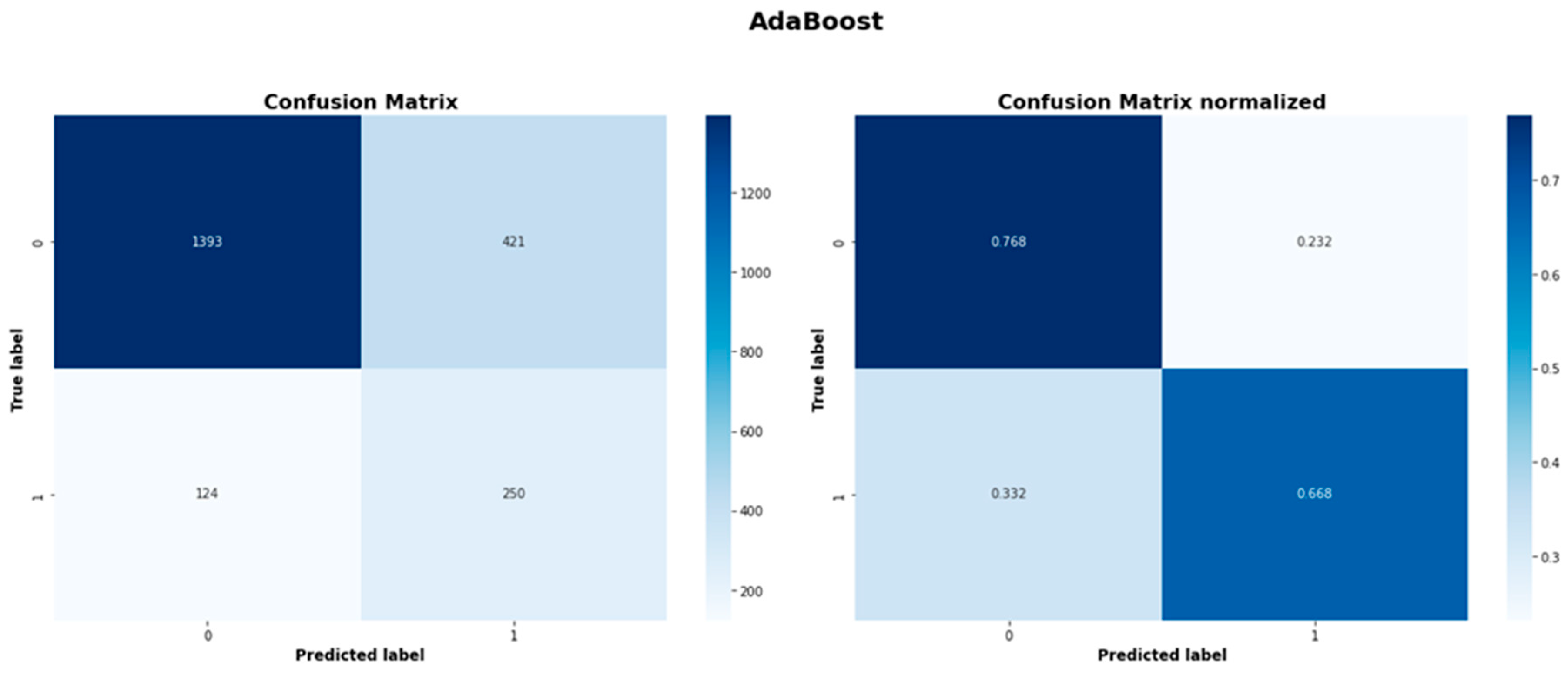
Figure A9.
MultinomialNB model confusion matrices.
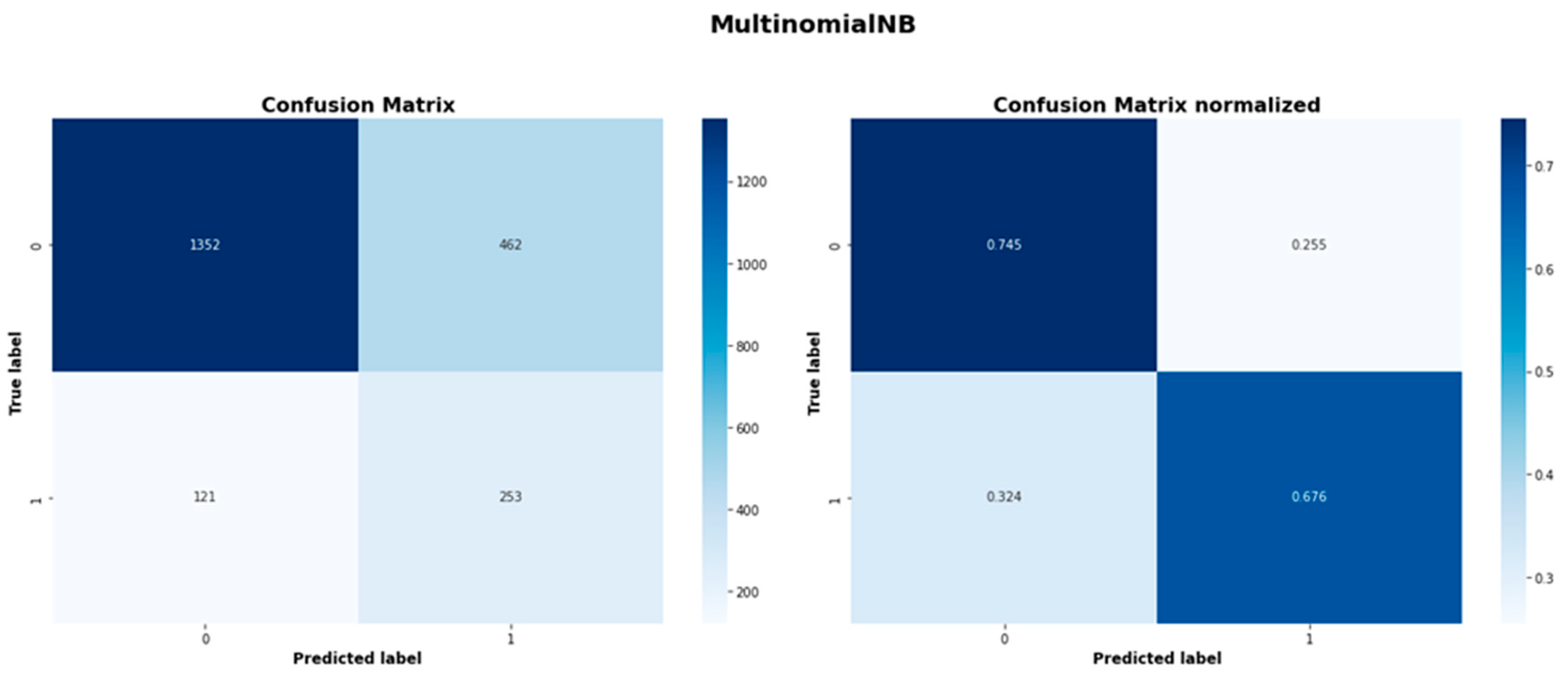
Figure A10.
Balanced Bagging MultinomialNB model confusion matrices.
References
- Commission Recommendation of 6 May 2003 concerning the definition of micro, small and medium-sized enterprises (notified under document number C(2003) 1422), Official Journal L 124 , 20/05/2003 P. 0036 – 0041, https://eur-lex.europa.eu/eli/reco/2003/361/oj.
- Chonsawat, N., & Sopadang, A. (2020). Defining SMEs’ 4.0 Readiness Indicators. Applied Sciences, 10(24), 8998. [CrossRef]
- Cusolito, A. P., Dautovic, E., & McKenzie, D. (2021). Can government intervention make firms more investment-ready? A randomized experiment in the Western Balkans. Review of Economics and Statistics, 103(3), 428–442. [CrossRef]
- Douglas, E. J., & Shepherd, D. A. (2002). Exploring investor readiness: Assessments by entrepreneurs and investors in Australia. Venture Capital, 4(3), 219–236. [CrossRef]
- Du, J., & Rada, R. (2010). Machine learning and financial investing. In Handbook of Research on Machine Learning Applications and Trends: Algorithms, Methods, and Techniques (pp. 375–398). IGI Global. [CrossRef]
- Dumitrescu, E., Hué, S., Hurlin, C., & Tokpavi, S. (2021). Machine learning or econometrics for credit scoring: Let’s get the best of both worlds. HAL Working Paper hal-02507499. Available at: https://hal.archives-ouvertes.fr/hal-02507499.
- European Central Bank (ECB) (2023). Survey on the Access to Finance of Enterprises (SAFE) Dataset. Retrieved from https://www.ecb.europa.eu/stats/ecb_surveys/safe/html/data.en.html.
- Fellnhofer, K. (2015). Literature review: Investment readiness level of small and medium-sized companies. International Journal of Managerial and Financial Accounting, 7(3/4), 268–284. [CrossRef]
- Friedman, J. H. (2001). Greedy function approximation: A gradient boosting machine. The Annals of Statistics, 29(5), 1189–1232. [CrossRef]
- Friedman, J. H. (1999). Stochastic Gradient Boosting. Technical Report. Stanford University.
- Khan, A. H., Shah, A., Ali, A., Shahid, R., Zahid, Z. U., Sharif, M. U., Jan, T., & Zafar, M. H. (2023). A performance comparison of machine learning models for stock market prediction with novel investment strategy. PLOS ONE, 18(9), e0286362. [CrossRef]
- Li, M. (2023). Financial investment risk prediction under the application of information interaction Firefly Algorithm combined with Graph Convolutional Network. PLOS ONE, 18(9), e0291510. [CrossRef]
- Mason, C. M., & Harrison, R. T. (2001). "Investment readiness": A critique of government proposals to increase the demand for venture capital. Regional Studies, 35(7), 663–668. [CrossRef]
- Mason, C. M., & Kwok, J. (2010). Investment readiness programmes and access to finance: A critical review of design issues. Working Paper 10-03, Hunter Centre for Entrepreneurship, University of Strathclyde.
- Mullainathan, S., & Spiess, J. (2017). Machine learning: An applied econometric approach. Journal of Economic Perspectives, 31(2), 87–106. [CrossRef]
- Okfalisa, et al. (2021). Measuring the effects of different factors influencing the readiness of SMEs towards digitalization: A multiple perspectives design of decision support system. Decision Science Letters, 10, 425–442. [CrossRef]
- Owen, R., Botelho, T., Hussain, J., & Anwar, O. (2023). Solving the SME finance puzzle: An examination of demand and supply failure in the UK. Venture Capital, 25(1), 31–63. [CrossRef]
- Pirola, F., Cimini, C., & Pinto, R. (2020). Digital readiness assessment of Italian SMEs: a case-study research. Journal of Manufacturing Technology Management, 31(5), 1045–1083. [CrossRef]
- Shobana, G., & Umamaheswari, K. (2021). Forecasting by machine learning techniques and econometrics: A review. In Proceedings of the Sixth International Conference on Inventive Computation Technologies (ICICT 2021). IEEE Xplore.
- Vasilescu, L. G. (2009). ‘Investment readiness’—aligning capital demand and supply. [Details needed from original publication].
- World Bank (2023). Small and Medium Enterprises (SMEs) Finance – Improving SMEs’ access to finance and finding innovative solutions to unlock sources of capital. Retrieved from: https://www.worldbank.org.
- Zana, D., & Barnard, B. (2019). Venture capital and entrepreneurship: The cost and resolution of investment readiness. SSRN Electronic Journal. Available at SSRN: . [CrossRef]
- Norvig, Russel (2020). Artificial Intelligence. A Modern Approach (4rth Edition) Pearson Series.
- Cover, T.M., & Hart, P.E. (1967). Nearest neighbor pattern classification. IEEE Trans. Inf. Theory, 13, 21-27.
- L. Breiman. (2001) Random Forests, Machine Learning, 45(1), 5-32.
- Cortes, C., & Vapnik, V. (1995). Support-vector networks. Machine Learning, 20(3), 273–297.
- Cox, D.R. (1958) The regression analysis of binary sequences. Journal of the Royal Statistical Society: Series B (Methodological), 20(2), pp.215–232.
- Freund, Y., & Schapire, R.E. (1997). A decision-theoretic generalization of on-line learning and an application to boosting. European Conference on Computational Learning Theory.
- Liu, X., Wu, J., & Zhou, Z. (2009). Exploratory Undersampling for Class-Imbalance Learning. IEEE Transactions on Systems, Man, and Cybernetics, Part B (Cybernetics), 39, 539-550.
- Breiman, L. (1996). Bagging predictors. Machine Learning, 24(2), 123–140.
- C.D. Manning, P. Raghavan and H. Schuetze (2008). Introduction to Information Retrieval. Cambridge University Press, pp. 234-265.
- Brodersen, K.H.; Ong, C.S.; Stephan, K.E.; Buhmann, J.M. (2010). The balanced accuracy and its posterior distribution. Proceedings of the 20th International Conference on Pattern Recognition, 3121-24.
- Gogas, P.; Papadimitriou, T.; Sofianos, E. (2019) Money Neutrality, Monetary Aggregates and Machine Learning. Algorithms, 12,137.
- Peykani, P., Peymany Foroushany, M., Tanasescu, C., Sargolzaei, M., & Kamyabfar, H. (2025). Evaluation of Cost-Sensitive Learning Models in Forecasting Business Failure of Capital Market Firms. Mathematics, 13(3), 368. ECB Data References: European Central Bank (2023). Survey on the Access to Finance of Enterprises (SAFE). Retrieved from: https://www.ecb.europa.eu/stats/ecb_surveys/safe/html/data.en.html. ECB (2023). SAFE Methodology Documentation. Retrieved from: https://data.ecb.europa.eu/data/datasets/SAFE/structure. ECB (2023). Dataset Structure Documentation. Retrieved from: https://data.ecb.europa.eu/data/datasets/SAFE/structure. ECB (2023). SAFE Data Information. Retrieved from: https://data.ecb.europa.eu/data/datasets/SAFE/data-information. [CrossRef]
Figure 7.
Gradient Boosting ROC Curve.
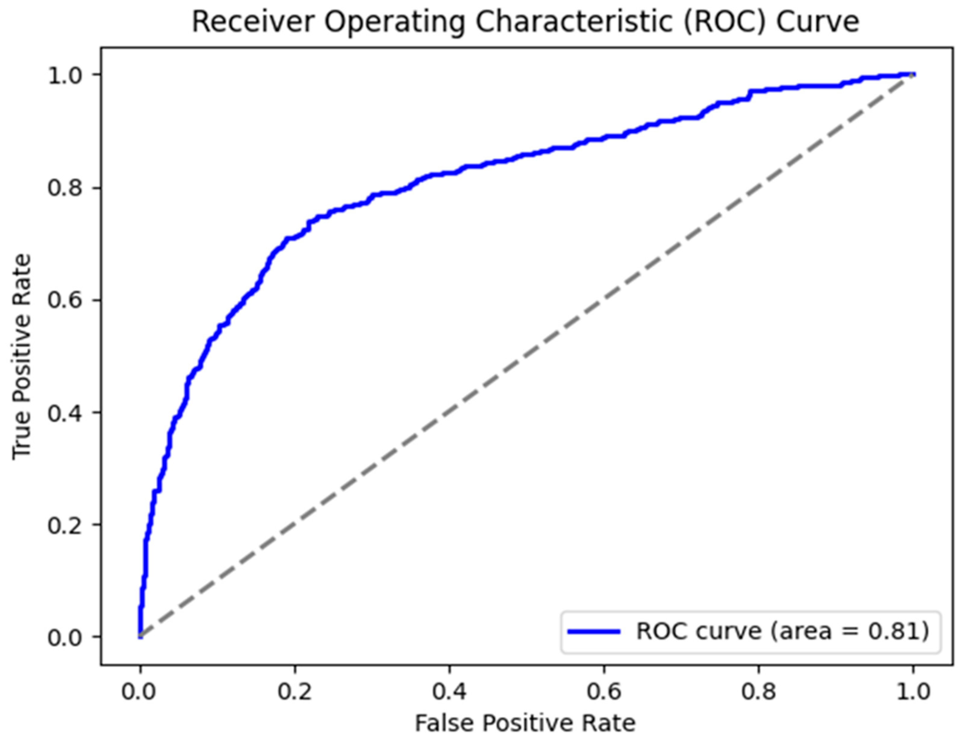
Figure 8.
Gradient Boosting Confusion Matrix.
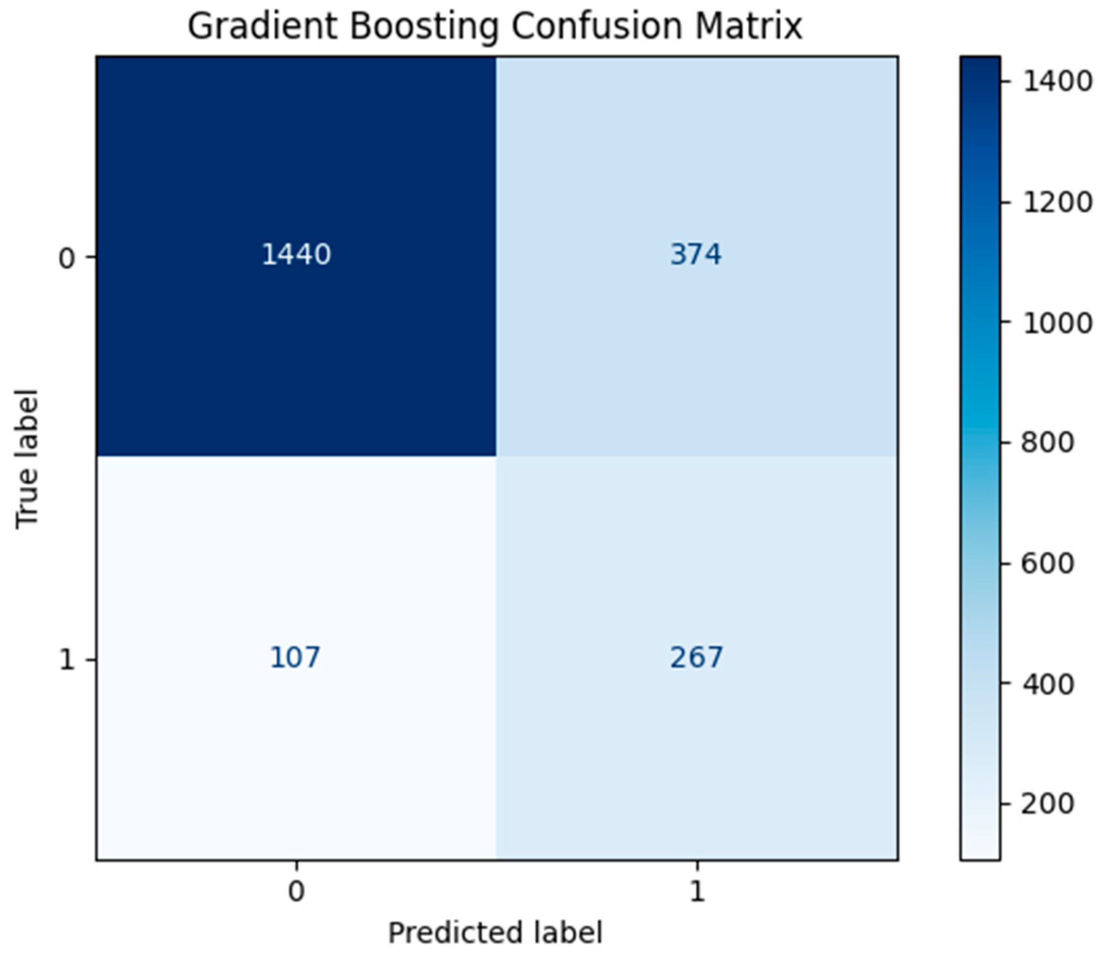
Figure 9.
Gradient Boosting Confusion Matrix normalized.
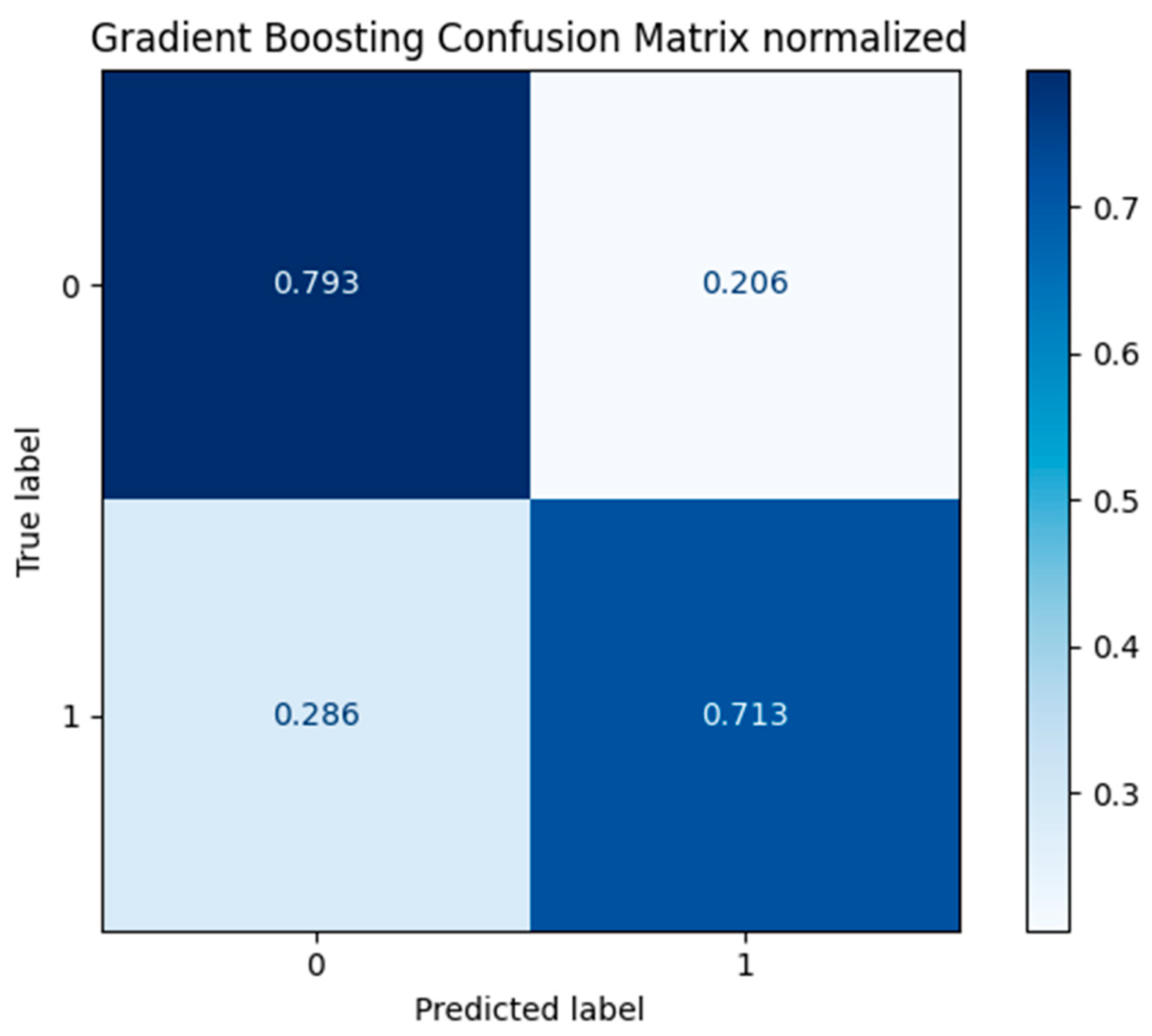
Figure 10.
Gradient Boosting Variable Importance Plot.
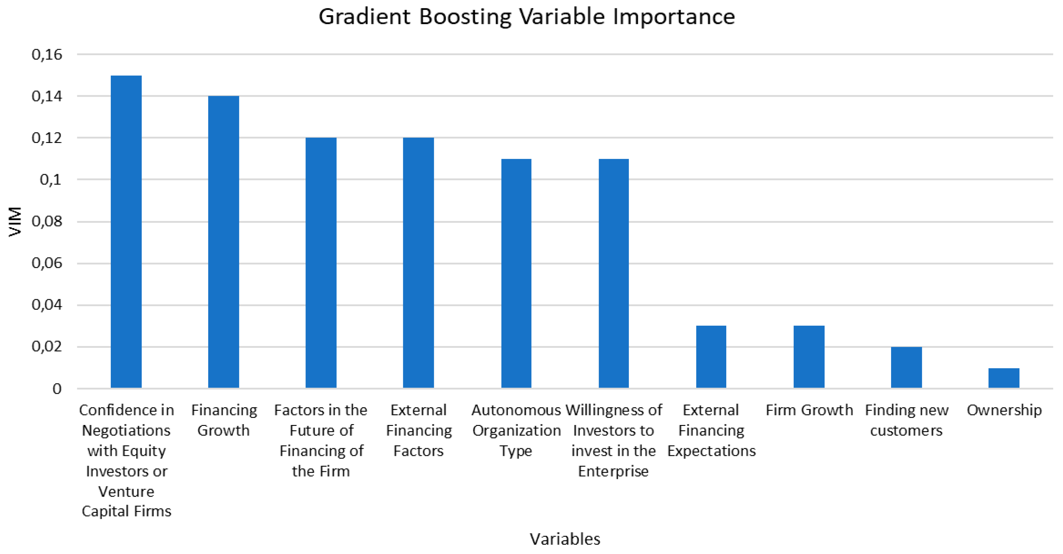
Table 1.
Comparison of models based on False Positives (FP), False Negatives (FN) and Total Misclassification Cost (TMC).
Table 1.
Comparison of models based on False Positives (FP), False Negatives (FN) and Total Misclassification Cost (TMC).
| Model | FP | FN | TMC |
| Gradient Boosting | 438 | 94 | 908 |
| Logistic Regression | 379 | 107 | 914 |
| Easy Ensemble Classifier | 409 | 103 | 924 |
| Random Forest | 441 | 99 | 936 |
| AdaBoost | 386 | 111 | 941 |
Disclaimer/Publisher’s Note: The statements, opinions and data contained in all publications are solely those of the individual author(s) and contributor(s) and not of MDPI and/or the editor(s). MDPI and/or the editor(s) disclaim responsibility for any injury to people or property resulting from any ideas, methods, instructions or products referred to in the content. |
© 2025 by the authors. Licensee MDPI, Basel, Switzerland. This article is an open access article distributed under the terms and conditions of the Creative Commons Attribution (CC BY) license (http://creativecommons.org/licenses/by/4.0/).
Copyright: This open access article is published under a Creative Commons CC BY 4.0 license, which permit the free download, distribution, and reuse, provided that the author and preprint are cited in any reuse.


