
Submitted:
05 July 2025
Posted:
07 July 2025
You are already at the latest version
Abstract
Understanding and modeling the flow of information in human societies is essential for capturing phenomena such as polarization, opinion formation, and misinformation diffusion. Traditional agent-based models often rely on simplified behavioral rules that fail to capture the nuanced and context-sensitive nature of human decision-making. In this study, we explore the potential of Large Language Models (LLMs) as data-driven, high-fidelity agents capable of simulating individual opinions under varying informational conditions. Conditioning LLMs on real survey data from the 2020 American National Election Studies (ANES), we investigate their ability to predict individual-level responses across a spectrum of political and social issues. Using Jensen–Shannon distance to quantify divergence in opinion distributions and F1-score to measure predictive accuracy we compare LLM-generated simulations to those produced by traditional Random Forest models. While performance at the individual level is comparable, LLMs consistently produce aggregate opinion distributions closer to the empirical ground truth. These findings suggest that LLMs offer a promising new method for simulating complex opinion dynamics and modeling the probabilistic structure of belief systems in computational social science.
Keywords:
LLM
; random forests
; Jensen–Shannon divergence
; public opinion simulation
; social sciences
1. Introduction
Survey research has long been a cornerstone of social science, political science, and policy-making, providing critical insights into public opinion, voting behavior, and social attitudes. However, traditional surveys face increasing challenges: they are costly, time-consuming, and burden respondents with long questionnaires, all while suffering from declining response rates and concerns about data reliability. These limitations motivate the exploration of computational methods that could complement or extend survey research, particularly through the use of artificial intelligence.
Large Language Models (LLMs) represent a promising avenue for this purpose. Trained on vast human-written corpora, LLMs capture not only grammatical structure and world knowledge but also complex patterns of human beliefs, biases, and associations [1,2]. Many recents studies focus on the consequences of these biases and how to mitigate them [3,4]. On the other hand, recent studies have shown that, when properly conditioned, LLMs can simulate nuanced group-level opinions by leveraging these same biases they encode [5,6]. This has led to the emergence of “silicon sampling” methodologies, where LLMs are employed as synthetic survey respondents to replicate human-like patterns of political and social beliefs. Despite this progress, critical questions remain about the granularity at which LLMs can simulate opinions—particularly whether they can accurately replicate individual-level responses, how large these LLMs need to be, and how different types of background information affect their performance.
In this study, we address these questions by proposing a framework for simulating public opinion using LLMs conditioned on structured survey data. Specifically, we use the 2020 American National Election Studies (ANES) dataset to build “backstories” for individual respondents, categorizing their attributes into three distinct groups: Demographic, Attitudinal and Political Orientation, and Moral and Social Values. By selectively providing the LLM with different categories of variables, we investigate how the amount and type of background information impacts its ability to simulate individual survey responses across a range of political and social topics.
Our research seeks to answer the following questions:
- How accurately can an LLM (Gemma3 12B) simulate individual responses to diverse opinion questions based on structured ANES backstory data?
- How does the type of information provided (Demographic, Attitudinal, Moral) influence the simulation accuracy? Which combinations of variable types are most effective?
- How does the LLM’s performance compare to a standard machine learning classifier (Random Forest) trained on the same data and task?
- How does the LLM’s ability to select relevant variables within a pool affect prediction accuracy?
- How does simulation accuracy vary across different socio-political topics?
To benchmark the performance, we compare the LLM’s predictions against real survey responses using the F1-score and Cramer’s V for individual-level accuracy and Jensen–Shannon distance (JSD) for distributional similarity. Notably, while the LLM performs comparably to Random Forests on individual-level F1-scores, it outperforms them in capturing the distributional patterns of opinions across most topics. This suggests that even moderately sized LLMs, like Gemma3 12B, can serve as powerful tools for cost-effective and scalable simulations of public opinion at a collective level.
Our main contributions are as follows:
- We propose a new framework for conditioning LLMs on structured backstory variables from public survey data to simulate individual and collective opinions.
- We systematically analyze the impact of different types and combinations of background information on simulation accuracy.
- We directly compare LLM performance against traditional machine learning methods on the same survey prediction tasks.
- We demonstrate the viability of LLMs as synthetic populations for simulating public opinion distributions, opening new avenues for low-cost and scalable survey research.
The paper proceeds by first reviewing related work on LLMs and opinion simulation, followed by a detailed description of our methodology and experimental design. We then present each simulation in detail before discussing the main results, limitations, and future directions.
2. Related Work
LLMs have demonstrated remarkable capabilities in generating coherent and contextually appropriate text. These models, trained on vast amounts of data, can simulate human-like responses, making them valuable tools in various applications, including synthetic surveying and social network simulations.
Recent research has increasingly explored the potential of LLMs to simulate aspects of human behavior. Several studies examine how LLMs reflect human cognitive biases, replicate patterns of human error in reasoning, or capture nuanced differences across demographic groups [7,8,9]. While much of this work focuses on evaluating LLMs’ ability to mimic human responses at an aggregate or cognitive task level, fewer studies have addressed the challenge of simulating individual-level opinion patterns based on structured background information. This section reviews some works that are closely related to our own, examining their behavior and limitations. We organize these works into three categories—Persona Simulation, LLMs in Social Science and Virtual Surveys—while acknowledging the significant overlap between them.
2.1. Persona Simulation
Recent work has explored using LLMs to create virtual agents or characters with coherent personalities and behaviors. For example, [10] introduced Generative Agents: language-model driven software agents with memory, planning, and reflection components that wake up, cook breakfast, head to work, notice news, form opinions, and coordinate events in a simulated town. In evaluation these agents exhibited believable individual and emergent social behaviors (e.g. planning a community party via invitation chains), demonstrating the potential of LLMs to simulate not only isolated responses but rich social interactions.
Other work has focused on endowing LLMs with more detailed character traits. In [11] the authors trained a “CharacterBot” on the collected writings of Lu Xun (a Chinese author) to capture his worldview and ideology. Their multi-task fine-tuning yields outputs that better preserve linguistic style and ideological perspective than simpler methods. Similarly, [12] construct the LifeChoice benchmark from novels to test if LLMs can predict characters’ decisions; they find state-of-the-art LLMs achieve promising accuracy, yet substantial room for improvement remains.
In human–computer interaction, [13] built PersonaFlow, an LLM-based system that simulates multiple expert personas (e.g. chemist, political scientist) during a brainstorming session. They report that interacting with several simulated experts improves the relevance and creativity of ideas, though it raises concerns about over-reliance and biases. Across these studies, a common limitation is that LLM-generated personas can oversimplify or stereotype real human variability. In [14] the authors noted that LLM-based demographic simulations often produce “caricatures” – excessively stereotyped or homogenized personas – and they propose metrics to quantify lack of individuation or exaggeration in model outputs. In general, current persona models require extensive curated data or prompt engineering and may fail to generalize beyond the studied characters.
2.2. LLMs in Social Science Experiments
In [15] the authors introduce the concept of Turing Experiments (TEs), a novel method to evaluate the zero-shot simulation capabilities of LLMs. In TEs, models are prompted to generate text transcripts simulating human responses across various experimental settings, offering insight into which human behaviors LLMs can replicate. The authors conducted four TEs across distinct domains: behavioral economics, psycholinguistics, social psychology and collective intelligence. Their results show that LLMs can capture meaningful human-like behavioral patterns, often with higher fidelity in larger models. However, they also highlight important challenges, including potential contamination from training data, the risk of prompt-induced biases, and ethical concerns in simulating sensitive aspects of human behavior. Overall, TEs provide a valuable tool for exploring how LLMs internalize and reflect complex social and cognitive behaviors, while underscoring the need for careful experimental design and interpretation.
Other work has adapted LLMs to field settings: In [16] the authors created an automated pipeline to extract information from 319 published field experiments (economics/social science) and prompt GPT-4 to choose outcome predictions; they achieve roughly 78% accuracy overall, though performance is highly uneven (e.g. worse for studies on gender or non-Western contexts). Finally, [17] introduce SocioVerse, a synthetic world built from 10 million “user profiles” and LLM-driven agents. In domains of politics, news, and economics, SocioVerse’s agents collectively reproduce population dynamics (e.g. election outcomes, public opinion shifts) while preserving diversity of attitudes.
These modeling efforts suggest that LLMs offer a promising new tool for social science: they can accelerate hypothesis testing and policy exploration without real subjects (reducing cost and ethical constraints) [18]. However, existing systems face clear limitations. LLMs ultimately rely on patterns in their training data, so their “inferences” may reflect historical and linguistic biases. They tend to underperform out-of-distribution or minority scenarios [19] and can produce overly confident or uniform answers compared to diverse human behavior [15]. Experts therefore caution that LLM-based simulations should be used cautiously and primarily for exploratory research, with repeated runs and careful variability analysis.
2.3. Virtual Surveys and Synthetic Respondents
Another emerging line of work treats LLMs as virtual survey participants, generating synthetic responses under given demographic profiles, which closely relates to our own work.
In [5] the authors introduce a framework for analyzing whose opinions LLMs reflect when responding to subjective questions across various topics, ranging from religion to science. The authors create OpinionQA, a dataset based on high-quality public opinion polls that allows for evaluating how LLM opinions align with those of 60 US demographic groups. In their primary analysis, the authors directly asked the LLMs the survey questions without any demographic-specific prompting or roleplaying instructions. This revealed a substantial misalignment between views expressed by current LLMs and those of US demographic groups. In their “steerability” experiments, most models do tend to become better-aligned with a specific group when prompted to behave like it, however, these improvements are modest. Here, we should note that the authors focused on demographic traits to condition the models. In contrast, our work goes further by incorporating attitudinal and moral dimensions into the respondent profiles. As we will demonstrate, this richer modeling helps explain why prior work observed only limited steerability: demographic factors alone are often insufficient to capture the full complexity of human opinions.
In [6] the authors introduce the concept of silicon sampling, proposing that LLMs like GPT-3 can serve as effective surrogates for human respondents in social science research. Their key idea is that “algorithmic bias” in LLMs is not a flaw but reflects fine-grained, demographically correlated patterns that can be systematically leveraged. In their study, the authors condition GPT-3 on thousands of real socio-demographic backstories drawn from large U.S. surveys, generating “silicon individuals” to simulate tasks such as vote choice prediction and answering closed-ended survey questions. While their work provides strong evidence that GPT-3 can simulate aggregate human responses when conditioned on demographic variables, it primarily focuses on traits such as race, gender, age, and political affiliation.
In [20] the authors probed ChatGPT-4 by assigning it demographic profiles from the World Values Survey and ANES. GPT-4 reproduces many cultural differences and “in-sample” response patterns across U.S. and Chinese subgroups, and even produced correct forecasts for the 2024 U.S. presidential election. However, it shows limitations on value-sensitive questions and an overall tendency to homogenize responses: subtle prompt phrasing or demographic details can substantially affect answers. In [21] the authors conducted a multi-country test by prompting GPT variants, Llama2, etc., to answer items from the European Social Survey on politics and democracy. They found that with a few relevant examples (“few shot prompts”) LLMs generate highly realistic answers, but in zero-shot mode (no examples) performance degrades markedly. Collectively these studies find that LLMs can simulate group-level opinion distributions, but major challenges and questions remains. In the next sections, we describe our approach to addressing the questions posed in the Introduction, developing a persona construction strategy that moves beyond demographic attributes to incorporate attitudinal and social values.
3. Materials and Methods
The ANES (American National Election Studies) is a respected research organization founded in 1948 that conducts comprehensive pre- and post-election surveys in the United States. These surveys collect extensive data on voter behavior, political attitudes, and public opinion, creating valuable datasets for social science researchers. In the next section we describe in detail the subset of the ANES 2020 dataset that we used in our work.
3.1. ANES 2020 dataset
The ANES 2020 dataset contemplates interviews with respondents between August 18, 2020, and November 3, 2020, being the primary data source for comprehending the American public opinion. The dataset includes demographic, social and behavioral information, including responses to presidential votes and political surveys. The dataset also features re-interviews with 2016 ANES respondents, and has samples from the 2020 pre-election and post-election periods.
In our work we focus exclusively on respondents from the 2020 pre-election sample, excluding the ANES 2016 respondents as well as post-election samples. We then select two groups of variables: the first we will denote by backstory variables, the second simply by topics. The backstory variables are the set of 25 variables that can be used to compose the “persona profile” of our virtual person. The topics are a set of 10 questions that this virtual person will answer when roleplayed by the LLM. We also group the backstory variables into three distinct groups: Demographic (D), Attitudinal and Political Orientation (A), and Moral and Social Values (M). For brevity, we often refer to the last two groups simply as “Attitudinal” and “Moral” variables, respectively.
Table 1, Table 2 and Table 3 present the response options available to survey participants. The interpretation of the Demographic and Attitudinal variables is self-explanatory. Among the Social Values variables, the “Preferred Child Trait” item asks respondents to select the child characteristic they value most from the provided options. The “Birthright Citizenship End” variable measures how strongly respondents favor or oppose ending automatic citizenship for children of unauthorized immigrants. Variables prefixed with “Discrimination” gauge respondents’ perceptions regarding the prevalence of specific types of discrimination at the time of the survey. The “Historic Racism Impact” item assesses respondents’ agreement with the statement that generations of slavery and discrimination have created conditions that make life more difficult for Black Americans. Table 4 shows the topics we are interested in.
For the topics Climate Change and Current Economy (marked with “*”), the original survey presented 5 choices. We remapped them in the following way: for Climate Change, options “A little” and “A moderate amount” were collapsed into “A little”, and options “A lot” and “A great deal“ were collapsed into “A lot”. For Current Economy, options “Very Good” and “Good” were collapsed into “Good”, and options “Bad” and “Very Bad“ were collapsed into “Bad”. This improves interpretability and ensure sufficient sample sizes across response categories, while retaining the substantive distinctions between low and high concern or between positive and negative evaluations [22]. All other topics are presented exactly as they appear in the survey.
3.2. Data Assembling and Splitting
Each topic in our study is treated as an independent modeling task. For a given experiment, the input dataset consists of a specific set of backstory variables along with the specific topic variable as the prediction target. Each row of the dataset corresponds to a single survey respondent, fully characterized by their backstory and topic-specific response.
Since we aim to compare the performance of LLMs against a traditional Random Forest (RF) classifier, it is essential that both models are evaluated on the same validation sets. To ensure fairness and maximize robustness, we adopt a 3-fold cross-validation strategy: in each fold, approximately 33% of the data is held out for validation, with the remaining 67% used for training (only for the RF). This procedure guarantees that all data points are used for validation exactly once, reducing variance and minimizing potential biases. All reported performance metrics are computed as the simple average across the three validation folds. Figure 1 illustrates this schema.
It is important to highlight again that no fine-tuning or training is performed on the LLM; it uses only the backstory information at inference time. Thus, the training data is utilized exclusively by the RF model. Lastly, respondents with missing data in any relevant fields were excluded from the analysis to maintain consistency across models.
3.3. Evaluation Metrics Statistical Analysis
To quantify the statistical uncertainty of our reported performance metrics (F1-score, JSD, Cramér’s V) and the differences between models or experimental conditions, we employed a non-parametric bootstrap procedure. For each primary metric averaged across the 3 cross-validation folds, B=1000 bootstrap iterations were performed. In each iteration, (prediction, true label) pairs were resampled with replacement from each fold’s original validation set (maintaining original fold sample sizes). The metric was calculated for these resampled data within each fold, and these three fold-level metrics were then averaged to produce one bootstrap estimate of the mean cross-validated metric. This process yielded a distribution of 1000 bootstrap estimates for each reported mean metric or mean difference. From these distributions, 95% confidence intervals (CIs) were derived using the percentile method (i.e., the 2.5th and 97.5th percentiles). Differences or gains were considered statistically significant at the p < 0.05 level if their corresponding 95% CI did not include zero. In the main text tables we mark the significant values with an asterisk (*). The full CI data can be found in the Appendix.
4. Results
4.1. Experimental Sequence
In the next sections we conduct four sequential experiments to evaluate and compare model performance. We begin by establishing a LLM baseline against naive models, using limited profile information (Exp 1). We then examine how access to more comprehensive variable pools affects model behavior (Exp 2). In the third experiment, we evaluate the model’s capacity for autonomous feature selection (Exp 3). Finally, we present the head-to-head comparison under identical conditions to isolate each model’s distinct capabilities (Exp 4).
4.2. Experiment 1 - Random and Constant Model Baselines
Before evaluating model accuracy or variable grouping effects, we establish a performance baseline using two naive models: a Random Model and a Constant Model. These serve as essential lower bounds for interpreting the behavior of more advanced models. For all experiments in this work we use Google’s Gemma3 12B, a compact yet capable LLM with 12 billion parameters.
The Random Model simulates a respondent who selects answers uniformly at random, representing a performance floor with no reliance on input features. The Constant Model always predicts the most frequent class from the training data, reflecting population-level bias but ignoring respondent variation. This is especially relevant in imbalanced datasets, where majority-class predictions can appear deceptively strong.
These baselines help determine whether the LLM captures meaningful patterns or merely mimics simple heuristics. To keep the this benchmark experiment as simple and interpretable as possible, we constrain the LLM to select only one backstory variable from each of the three groups. For each topic, the model selects the most predictive variable per group using its internal knowledge. These are then used to construct the virtual respondent’s prompt. This setup provides a minimal yet structured input, enabling consistent evaluation across topics. Prompt templates for this experiment are included in the Appendix. We also note that for all LLM experiments the temperature parameter was held fixed at a value of 0.3. A low temperature of 0.3 was chosen to reduce randomness and encourage the model to produce the most probable, deterministic response based on the provided persona. Previous work like [6] found the temperature parameter to produce stable results, but since our work uses a different setting, we plan to study temperature effects more deeply in future works.
As shown in Table 5, the LLM consistently and substantially outperforms both the Random and Constant baseline models across all 10 survey topics and all three evaluation metrics (F1-score, Jensen-Shannon Distance (JSD), and Cramér’s V). For instance, on the “Climate Change” topic, the LLM achieved an F1-score of 0.59, compared to 0.36 for the Random model and 0.41 for the Constant model. Similarly, its JSD of 0.21 was markedly better (lower) than the Random model’s 0.29 and the Constant model’s 0.51, indicating superior distributional alignment. The Cramér’s V also showed a clear advantage for the LLM (e.g., 0.41 for “Climate Change” vs. 0.04 for Random; Constant model has no basis for Cramér’s V calculation as it doesn’t use input features). The 95% Confidence Intervals for Experiment 1 results can be found in the Appendix.
This pattern of LLM superiority over the naive baselines holds true across all topics. For example, for “Gay Marriage”, the LLM’s F1-score (0.68) and JSD (0.10) far exceeded those of the Random (F1: 0.38, JSD: 0.33) and Constant (F1: 0.59, JSD: 0.40) models. However, we point out two statistically significant exceptions: First, in the “Drug Addiction” topic, where the Constant model’s F1-score was slightly better (+0.02) due to class imbalance. In this case the LLM demonstrated a significantly better JSD (0.20 vs. 0.41), showcasing its superior ability to capture more than just the majority class. The second, in the “Refugee Allowing” topic, where the JS for the Random model was 0.15 better. Here, the LLM was better at both F1-score and Cramér’s V, suggesting that the variable selection made by the LLM for this specific topic was not good enough. This is confirmed in the next experiments, where the JS for the topic “Refugee Allowing” is significantly better than the one achieved by the Random model.
These results affirm that even with a highly constrained set of input variables, the LLM captures meaningful predictive patterns from the backstory information, performing well above chance and simple heuristics. This validates its potential for opinion simulation and sets the stage for exploring its capabilities with more comprehensive informational inputs in subsequent experiments.
4.3. Experiment 2 - Impact of Backstory Variable Categories on Simulation Accuracy
In Experiment 1 we established a performance baseline where the LLM was constrained to utilize a minimal set of information: one self-selected predictor variable from each of the three primary backstory categories, totaling at most three variables. Building upon this, in this section we investigate the potential performance gains and the differential impact achieved when the LLM has access to all variables in each of the seven distinct combinations of these “variable pools”.
The 25 backstory variables are grouped into three categories (Table 1, Table 2 and Table 3), resulting in seven combinations or “variable pools”. For each topic + variable pool, the LLM is explicitly instructed to use all variables from the pool to make predictions. The prompt templates can be found in the Appendix.
We also trained and evaluated RF classifiers on the exact same data. A separate RF classifier is trained for each topic + variable pool combination, using only the backstory variables from the given pool as input features and the corresponding topic survey response as the target. Both inputs and targets are encoded as integers. The training parameters for the RF classifiers are held constant across all experiments and are detailed in the Appendix.
In Table 6 through Table 9 we summarize the best performing models across variable pools, for each topic. Table 6 and Table 7 detail the peak F1-score, JSD, and Cramér’s V achieved by the Gemma3 12B LLM and the RF model, respectively, along with the specific variable pool yielding this optimal performance for each topic and metric. A noteworthy initial observation is that these optimal variable pools frequently differed between the LLM and RF for identical tasks, suggesting distinct information utilization strategies by each model. Table 8 quantifies the LLM’s performance gains in this experiment relative to the more constrained Experiment 1 baseline, while Table 9 directly compares the peak LLM performance against the peak RF performance. Pool names are abbreviated for space.
Analysis of the LLM’s optimal configurations (Table 6) reveals that variable pools incorporating Attitudinal (A) or Moral (M) attributes, or their combination (A+M), frequently yielded the best results across most topics and metrics. For instance, on the “Climate Change” topic, the A+M pool provided the LLM’s highest F1-score (0.70) and best JSD (0.15). As detailed in Table 8, these scores represented substantial F1 and JSD gains of 0.11 and 0.07, respectively, over the Experiment 1 baseline, indicating that richer psychological information significantly enhanced simulation accuracy for this topic. Conversely, for “Gay Marriage”, while the A pool yielded the LLM’s best F1-score (0.66), this was a slight decrease from the Experiment 1 baseline, and the JSD also showed a decline, suggesting the simpler Experiment 1 setup was more effective for these specific metrics, though Cramér’s V did see a marginal improvement.
No single variable pool proved universally optimal. While A or M variables were prevalent in high-performing configurations, Demographic (D) variables tended to contribute most effectively in combination with other types, particularly for topics with inherent demographic components like “Gender Role”. For distributional similarity (JSD), the A pool demonstrated broad effectiveness, notably achieving the largest JSD gain over the baseline (+0.26) for “Refugee Allowing”. The magnitude of these gains over the Experiment 1 baseline varied considerably; substantial JSD improvements were also seen for “Health Insurance Policy” (+0.17 with D+A pool) and “Race Diversity” (+0.14 with A pool). While providing more extensive backstory information in Experiment 2 generally benefited LLM performance, especially for JSD, the Experiment 1 baseline occasionally remained competitive or superior, highlighting a nuanced interplay between question type, evaluation metric, and the most pertinent conditioning information.
A direct comparison between the peak LLM performance and peak RF performance, with each model utilizing its respective optimal variable pool (Table 9), reveals distinct capabilities. The LLM consistently demonstrated superior or equal ability in matching overall opinion distributions, achieving a statistically better JSD on six out of ten topics. Particularly notable JSD advantages for the LLM were observed for "Drug Addiction" (+0.18) and "Gender Role" (+0.18), underscoring its proficiency in capturing nuanced collective response patterns.
Regarding individual prediction accuracy (F1-score), the comparison was more balanced. The RF model often achieved a marginally higher peak F1-score, with a more pronounced advantage for “Gun Regulation” where its F1-score was 0.08 points higher than the LLM’s. Similarly, for associative strength (Cramér’s V), the RF model exhibited a clear superiority for “Gun Regulation” (-0.19) and “Race Diversity” (-0.17), while the LLM held a slight edge for “Drug Addiction” (+0.06), with minimal differences on other topics.
Experiment 2 demonstrates that while an RF classifier can achieve comparable or superior peak individual prediction accuracy (F1-score) and associative strength (Cramér’s V) on certain topics when operating with its optimal variable set, the Gemma3 12B LLM generally excels at replicating the distributional characteristics of survey responses (JSD). This distinction highlights their differing strengths: RF for robust predictive power on specific tasks, and LLMs for their nuanced capacity to simulate finer-grained collective opinion structures.
4.4. Experiment 3 - Impact of LLM-Driven Feature Selection on Simulation Accuracy
Unlike Experiment 2, where the LLM utilized all variables within a given pool, in this experiment the LLM was first prompted to select only the variables it deemed most relevant for prediction from each topic and variable pool combination. Only these self-selected variables were then used to construct the respondent’s profile for simulation. This approach offers a practical advantage in reducing prompt token count, leading to more efficient inference. The RF model results from Experiment 2, where the RF used its optimal variable pool, serve as a benchmark for comparison.
Table 10 details the peak performance of the Gemma3 12B LLM in Experiment 3 across all topics and metrics when employing this feature selection strategy, along with the variable pool from which features were selected. A comparison of these results with the LLM’s performance in Experiment 2 (Table 6, where all variables in the optimal pool were used), reveals nuanced effects of feature selection. For F1-score and Cramér’s V, the differences were generally marginal across most topics, often close to zero. However, for JSD, LLM-driven feature selection yielded notable improvements in distributional alignment for several topics. For instance, JSD for “Income Inequality” and “Race Diversity” improved by 0.08 and 0.05, respectively. This suggests that by focusing on a curated set of variables, the LLM can sometimes enhance its ability to replicate collective opinion patterns.
Nevertheless, the efficacy of this internal feature selection was not uniform. A striking instance is the “Health Insurance Policy” topic, where JSD worsened by 0.11 when feature selection was employed. This decline coincided with the optimal pool for JSD shifting from D+A in Experiment 2 to A+M in Experiment 3, suggesting that the LLM’s feature selection may have deprioritized or omitted the crucial health insurance demographic variable. This highlights a potential trade-off: while feature selection can enhance efficiency and, in some cases, improve JSD, it may occasionally overlook critical variables, particularly for topics with strong correlation to specific input features. The distribution of optimal variable pools also shifted in Experiment 3, with the D pool appearing more frequently as optimal for certain metrics compared to Experiment 2.
When comparing the peak LLM performance with feature selection against the peak RF performance from Experiment 2 (Table 11), the overall trends largely mirrored those observed in the Experiment 2 LLM vs. RF comparison. The LLM maintained its advantage in JSD for several topics, demonstrating strong distributional alignment. For example, for “Drug Addiction” the LLM with feature selection achieved a JSD improvement of 0.23 over the peak RF performance, and for “Gender Role”, the improvement was 0.15.
Conversely, for individual prediction accuracy (F1-score), the RF model from Experiment 2 often held a slight edge or performed comparably to the LLM with feature selection. For “Gun Regulation” the RF outperformed the LLM by 0.07 in F1-score. Similarly, for associative strength (Cramér’s V), the RF demonstrated stronger performance for “Gun Regulation” (-0.18) and “Race Diversity” (-0.18), while the LLM showed an advantage for “Drug Addiction” (+0.09).
In essence, allowing the LLM to perform feature selection can lead to more efficient inference and, in some instances, can refine its ability to capture distributional patterns (JSD). However, its performance relative to a well-configured RF model remains largely consistent with the trends observed without this explicit LLM feature selection step: the LLM excels in distributional similarity, while the RF often matches or slightly exceeds it in individual prediction accuracy on specific tasks.
4.5. Experiment 4: Head-to-Head Model Performance Across All Topic and Variable Pool Configurations
On both Experiments 2 and 3 we focused on identifying and comparing LLM and RF peak model performances across variable pools, which showed that optimal variable pools frequently differed between the LLM and RF for the same topic. In this section we present the direct comparison of these models under identical information conditions: for each topic we compare the performance under the same variable pool. To do this, we use the results from Experiment 2, since in this experiment the LLM utilizes all variables available within each pool, mirroring the RF’s input. This allows for a granular assessment of relative model strengths when the informational input is precisely matched.
The comparative performance is primarily visualized through heatmaps (Figure 2, Figure 3 and Figure 4) depicting the difference between LLM and RF scores for F1-score, Jensen-Shannon Distance (JSD), and Cramér’s V, respectively. In these figures, rows represent the survey topics and columns denote the seven variable pools. Cell values quantify the performance gap (LLM score - RF score for F1-score and Cramér’s V; RF JSD - LLM JSD for JSD), with positive values (e.g., blue shades) indicating LLM superiority for that specific topic-pool combination. As in previous experiments, an asterisk (*) denotes a difference for which the 95% bootstrap confidence interval does not include zero, indicating statistical significance (p < 0.05).
An examination of these heatmaps reveals distinct patterns in the relative performance of the Gemma3 12B LLM and the RF when given identical inputs from each variable pool.
For F1-score (Figure 2), the RF model generally demonstrates an advantage or performs comparably to the LLM across most topic-pool configurations. This is evidenced by the prevalence of neutral (light/white) or orange/red shades. For instance, on “Gun Regulation”, the RF consistently outperforms the LLM across all variable pools, with particularly strong advantages when using the D (Diff: -0.33), D+M (Diff: -0.34), and M (Diff: -0.31) pools. Similarly, for “Current Economy“, the RF shows better F1-scores with pools like A+M (Diff: -0.19) and D+A (Diff: -0.15). The LLM achieves comparable or slightly better F1-scores in isolated cells, such as for “Drug Addiction” with the D+A pool (Diff: +0.03) or “Gender Role” with the D+A+M pool (Diff: +0.02), but these instances are less frequent. This suggests that for individual prediction accuracy under these matched input conditions, the RF model often has an edge.
The JSD comparison (Figure 3) presents a more favorable outcome for the LLM. The LLM frequently achieves superior distributional similarity across a variety of topics and pools. Notably, for “Drug Addiction”, the LLM shows strong JSD advantages with the A (Diff: +0.23) and D+A (Diff: +0.22) pools. For “Gender Role”, the LLM also performs well with the A (Diff: +0.18) and D+A (Diff: +0.18) pools. Similar LLM advantages in JSD are seen for “Health Insurance Policy” with A, A+M, D+A, and D+A+M pools. However, the RF can still achieve better JSD in some cases, particularly when the D pool is used for topics like “Climate Change” (Diff: -0.24) or “Current Economy” (Diff: -0.33), and notably for “Gun Regulation” with the D pool (Diff: -0.39). This indicates that while the LLM often excels in JSD, its advantage is not universal and can be pool-dependent, with RF sometimes performing better especially with purely demographic information.
Regarding Cramér’s V (Figure 4), which measures associative strength, the RF model again tends to show stronger performance or parity in many topic-pool combinations. Negative values, indicating RF superiority, are prominent for “Gun Regulation” across all pools, with the largest differences seen with D+M (Diff: -0.33), D (Diff: -0.22), and A+M (Diff: -0.21). For “Race Diversity”, the RF also consistently outperforms the LLM. The LLM demonstrates a competitive or superior Cramér’s V for “Drug Addiction” across most pools (e.g., M pool, Diff: +0.07) and for “Health Insurance Policy” with the M pool (Diff: +0.11). However, for many other topic-pool cells, the differences are small or slightly favor the RF model.
This head-to-head comparison, where both models process the exact same variables from each pool, suggests that the RF model often exhibits superior or comparable performance in terms of F1-score and Cramér’s V. The Gemma3 12B LLM, however, frequently demonstrates an advantage in capturing the distributional nuances of survey responses, as measured by JSD, although this strength can also be influenced by the specific variable pool provided.
5. Conclusions
Our study investigated the capabilities of LLMs, specifically Gemma3 12B, to act as synthetic survey respondents, utilizing the 2020 ANES dataset. Our findings demonstrate that LLMs, when appropriately conditioned, serve as a potent tool for simulating public opinion, significantly outperforming naive baseline models even with minimal input.
A key contribution of our work is the detailed comparative analysis against traditional Random Forest classifiers and the nuanced exploration of different categories of backstory information—Demographic, Attitudinal and Political Orientation, and Moral and Social Values. We consistently found that while LLMs achieve individual-level prediction accuracy (F1-score) comparable to Random Forests, they notably excel in capturing the overall distributional patterns of opinions (as measured by Jensen-Shannon Distance) across a majority of socio-political topics. This superior performance in reflecting collective sentiment is particularly evident when LLMs are provided with richer combinations of attitudinal and moral variables, often surpassing the utility of demographic data alone. This highlights why previous studies focusing primarily on demographic conditioning may have observed limited steerability.
The research also explored the LLM’s inherent ability to discern relevant variables, showing that even when tasked with selecting a subset of features (Experiment 3), performance remained robust and, in some cases, JSD improved. This suggests a potential for more efficient prompting strategies, though with the caveat that crucial, topic-specific variables might occasionally be overlooked if not explicitly provided.
In direct head-to-head comparisons with Random Forests using identical input variable pools (Experiment 4), the pattern held: Random Forests often showed a slight edge or parity in F1-score and Cramér’s V, while the LLM maintained its advantage in distributional similarity (JSD). This underscores distinct strengths, with RFs suited for raw predictive power on individual responses and LLMs better at simulating the collective opinion landscape.
We hypothesize that these distinct strengths stem directly from the models’ training paradigms. The Random Forest is a discriminative model trained exclusively to find the optimal predictive pathways within the ANES sample, making it highly proficient at individual classification (F1-score, Cramér’s V). Conversely, the LLM leverages its vast pre-training on web-scale text, which has implicitly taught it the statistical distributions of beliefs and attitudes at a population level. This allows it to generate responses that better reflect the overall shape of public opinion, often leading to superior distributional accuracy (JSD).
In conclusion, our research substantiates the growing potential of LLMs as a valuable and scalable instrument for social science research. They offer a promising, cost-effective method to generate synthetic survey data, explore “silicon sampling”, and complement traditional survey methodologies, especially for understanding nuanced collective opinion patterns. While traditional machine learning models like Random Forests may retain advantages in specific individual prediction contexts, the demonstrated strength of LLMs in distributional modeling positions them as an important new tool for advancing our understanding of public opinion dynamics.
6. Limitations and Future Research
While this study provides strong evidence for the utility of LLMs in public opinion simulation, it is important to acknowledge its limitations. First, our analysis is centered on a single, small-sized open-source model, Gemma 3 12B. Performance and behavioral patterns may vary with different model architectures, sizes (e.g., larger proprietary models like GPT-4), or quantization methods. Future work should extend this comparative framework to a broader range of models to assess the generalizability of our findings.
Second, the findings are rooted in the 2020 American National Election Studies (ANES) dataset. The observed relationships between demographic, attitudinal, and moral variables are specific to the U.S. socio-political context of that time. The framework’s effectiveness in simulating public opinion in other cultures, political systems, or time periods requires explicit validation.
Finally, this work is confined to simulating responses for structured, multiple-choice survey questions. While our distributional metrics (JSD) show strong aggregate performance, there remains a risk that LLMs can generate “caricatures” that over-represent common statistical correlations rather than capturing the full spectrum of nuanced or atypical human beliefs. The ability to generate authentic, open-ended textual responses remains a key area for future exploration. These limitations highlight important directions for continued research, including cross-cultural validation and the development of more sophisticated metrics for assessing the qualitative authenticity of synthetic personas.
Author Contributions
Conceptualization, F.M. and P.P.; methodology, F.M.; software, F.M.; validation, F.M., P.P.; formal analysis, F.M. and P.P.; investigation, F.M.; resources, F.M.; data curation, F.M.; writing—original draft preparation, F.M.; writing—review and editing, F.M. and P.P.; visualization, F.M.; supervision, P.P.; project administration, P.P.; funding acquisition, P.P. All authors have read and agreed to the published version of the manuscript.
Funding
This research received no external funding.
Data Availability Statement
The code and data used in this study are publicly available at https://github.com/fernandotenorio/ANES_2020_survey_simulation.
Acknowledgments
F.M. thanks Instituto Presbiteriano Mackenzie for a graduate grant, and P.P.B. thanks the Brazilian agencies CNPq (Conselho Nacional de Desenvolvimento Científico e Tecnológico) for the research grant PQ 303356/2022-7, and CAPES (Coordenação de Aperfeiçoamento de Pessoal de Nível Superior) for the research grant STIC-AmSud (CAMA) no. 88881.694458/2022-01.
Conflicts of Interest
The authors declare no conflicts of interest.
Appendix A. Prompts
Appendix A.1. Baseline Feature Selection
|
You are a reasoning assistant trained to understand how personal characteristics shape beliefs and opinions. Your task is to analyze a set of variables describing individuals in the U.S. and select the variables most predictive of a person’s response to a survey question on the topic of {TOPIC}. Below are the variables grouped by theme and their descriptions. Demographic race: Self-identified race age: Age gender: Male or female income: Annual family income education: Education level occupation: Employment type city_rural: Identifies as urban or rural children: Number of children health_insurance: Has health insurance or not Attitudes & Political Orientation ideology: Political ideology (liberal, conservative, etc.) party: Political party affiliation interested_politics: Interested in politics or not trust_media: Trust in mainstream media science: Belief that people need help from experts to understand science vaccines_autism: Belief that vaccines cause autism religion_importance: How important religion is in the respondent’s life Moral Compass & Social Values child_trait: Most important child trait (e.g., obedience vs. self-reliance) death_penalty: Support or opposition to the death penalty birth_citizenship: View on banning birthright citizenship for children of undocumented immigrants children_sent_back: View on deporting children of undocumented immigrants discrimination_woman: Perceived discrimination against women black_discrimination: Perceived discrimination against Black people black_hist: Belief that past racism still affects Black Americans today gays_discrimination: Perceived discrimination against gay people muslins_discrimination: Perceived discrimination against Muslims Survey Question We want to predict the respondent’s answer to the following question: Question: {QUESTION} Answer choices: {ANSWER CHOICES} Instructions Based on your understanding of human behavior, select exactly one variable from each of the three groups above that you believe is the most predictive of how someone would respond to the question above. Respond only in this JSON format: { "selected_variables": ["variable_1", "variable_2", "variable_3"] } |
Appendix A.2. Variables Pool Feature Selection
|
You are a reasoning assistant trained to understand how personal characteristics shape beliefs and opinions. Your task is to analyze a set of variables describing individuals in the U.S. and select the variables most predictive of a person’s response to a survey question on the topic of {TOPIC}. Below are the variables grouped by theme and their descriptions. Demographic race: Self-identified race age: Age gender: Male or female income: Annual family income education: Education level occupation: Employment type city_rural: Identifies as urban or rural children: Number of children health_insurance: Has health insurance or not Attitudes & Political Orientation ideology: Political ideology (liberal, conservative, etc.) party: Political party affiliation interested_politics: Interested in politics or not trust_media: Trust in mainstream media science: Belief that people need help from experts to understand science vaccines_autism: Belief that vaccines cause autism religion_importance: How important religion is in the respondent’s life Moral Compass & Social Values child_trait: Most important child trait (e.g., obedience vs. self-reliance) death_penalty: Support or opposition to the death penalty birth_citizenship: View on banning birthright citizenship for children of undocumented immigrants children_sent_back: View on deporting children of undocumented immigrants discrimination_woman: Perceived discrimination against women black_discrimination: Perceived discrimination against Black people black_hist: Belief that past racism still affects Black Americans today gays_discrimination: Perceived discrimination against gay people muslins_discrimination: Perceived discrimination against Muslims Survey Question We want to predict the respondent’s answer to the following question: Question: {QUESTION} Answer choices: {ANSWER CHOICES} Instructions Based on your understanding of human behavior, select only the variables that are most predictive of how someone would respond to the question above. Favor clarity and precision over length. Respond only in this JSON format: { "selected_variables": ["variable_1", "variable_2", "..."] } |
Appendix A.3. Baseline Feature Selection: Gun Regulation Example
|
You are a reasoning assistant trained to understand how personal characteristics shape beliefs and opinions. Your task is to analyze a set of variables describing individuals in the U.S. and select the variables most predictive of a person’s response to a survey question on the topic of “Gun regulation”. Below are the variables grouped by theme and their descriptions. Demographic race: Self-identified race age: Age gender: Male or female income: Annual family income education: Education level occupation: Employment type city_rural: Identifies as urban or rural children: Number of children health_insurance: Has health insurance or not Attitudes & Political Orientation ideology: Political ideology (liberal, conservative, etc.) party: Political party affiliation interested_politics: Interested in politics or not trust_media: Trust in mainstream media science: Belief that people need help from experts to understand science vaccines_autism: Belief that vaccines cause autism religion_importance: How important religion is in the respondent’s life Moral Compass & Social Values child_trait: Most important child trait (e.g., obedience vs. self-reliance) death_penalty: Support or opposition to the death penalty birth_citizenship: View on banning birthright citizenship for children of undocumented immigrants children_sent_back: View on deporting children of undocumented immigrants discrimination_woman: Perceived discrimination against women black_discrimination: Perceived discrimination against Black people black_hist: Belief that past racism still affects Black Americans today gays_discrimination: Perceived discrimination against gay people muslins_discrimination: Perceived discrimination against Muslims Survey Question We want to predict the respondent’s answer to the following question: Question: Do you think the federal government should make it more difficult for people to buy a gun than it is now, make it easier for people to buy a gun, or keep these rules about the same as they are now? Answer choices: (1) More difficult (2) Easier (3) Keep these rules about the same Instructions Based on your understanding of human behavior, select exactly one variable from each of the three groups above that you believe is the most predictive of how someone would respond to the question above. Respond only in this JSON format: { "selected_variables": ["variable_1", "variable_2", "variable_3"] } |
Appendix A.4. Variables Pool Feature Selection: Gun Regulation Example
|
You are a reasoning assistant trained to understand how personal characteristics shape beliefs and opinions. Your task is to analyze a set of variables describing individuals in the U.S. and select the variables most predictive of a person’s response to a survey question on the topic of “Gun regulation”. Below are the variables grouped by theme and their descriptions. Demographic race: Self-identified race age: Age gender: Male or female income: Annual family income education: Education level occupation: Employment type city_rural: Identifies as urban or rural children: Number of children health_insurance: Has health insurance or not Attitudes & Political Orientation ideology: Political ideology (liberal, conservative, etc.) party: Political party affiliation interested_politics: Interested in politics or not trust_media: Trust in mainstream media science: Belief that people need help from experts to understand science vaccines_autism: Belief that vaccines cause autism religion_importance: How important religion is in the respondent’s life Moral Compass & Social Values child_trait: Most important child trait (e.g., obedience vs. self-reliance) death_penalty: Support or opposition to the death penalty birth_citizenship: View on banning birthright citizenship for children of undocumented immigrants children_sent_back: View on deporting children of undocumented immigrants discrimination_woman: Perceived discrimination against women black_discrimination: Perceived discrimination against Black people black_hist: Belief that past racism still affects Black Americans today gays_discrimination: Perceived discrimination against gay people muslins_discrimination: Perceived discrimination against Muslims Survey Question We want to predict the respondent’s answer to the following question: Question: Do you think the federal government should make it more difficult for people to buy a gun than it is now, make it easier for people to buy a gun, or keep these rules about the same as they are now? Answer choices: (1) More difficult (2) Easier (3) Keep these rules about the same Instructions Based on your understanding of human behavior, select only the variables that are most predictive of how someone would respond to the question above. Favor clarity and precision over length. Respond only in this JSON format: { "selected_variables": ["variable_1", "variable_2", "..."] } |
Appendix A.5. Survey
|
Roleplay the person below. The date is November 3, 2020. When questioned, answer just with the option number and nothing more. {SELECTED BACKSTORY VARIABLE 1.} {SELECTED BACKSTORY VARIABLE 2.} {...} {SELECTED BACKSTORY VARIABLE N.} Question: {QUESTION} Answer choices: {ANSWER CHOICES} My answer is |
Appendix A.6. Survey: Gun Regulation Example with all backstory variables
|
Roleplay the person below. The date is November 3, 2020. When questioned, answer just with the option number and nothing more. Racially, you are White. Ideologically, you are slightly conservative. Politically, you are not very strong Republican. Religion is moderately important in my life. You are 42 years old. You are a man. You are not at all interested in politics. Your total family income is $175,000-249,999. At the moment you do have health insurance. You have a Bachelor’s degree. Your employment is best described as working for a for-profit company or organization. You consider yourself a small-town person. You have two children. You believe that people need a lot of help from experts to understand science. You believe that most scientific evidence shows childhood vaccines do not cause autism. You have little trust in the media when it comes to reporting the news accurately and fairly. You believe that when it comes to obedience vs self-reliance, obedience is a more important trait for a child to have. You believe there is a moderate amount of discrimination against women in the US today. You favor a moderate amount that children of unauthorized immigrants do not automatically get citizenship if they are born in the US. You oppose a little that children of unauthorized immigrants who were brought to the US illegally and have lived here for at least 10 years should be deported. You disagree somewhat that generations of slavery and discrimination have created conditions that make it difficult for blacks to work their way out of the lower class. You believe there is a moderate amount of discrimination against blacks in the US today. You believe there is a moderate amount of discrimination against gays and lesbians in the US today. You believe there is a lot of discrimination against muslins in the US today. You favor the death penalty. Question: Do you think the federal government should make it more difficult for people to buy a gun than it is now, make it easier for people to buy a gun, or keep these rules about the same as they are now? Answer choices: (1) More difficult (2) Easier (3) Keep these rules about the same My answer is |
Appendix B. 95% Bootstrap Confidence Intervals for Performance Metrics
All estimates are based on bootstrap iterations.
Appendix B.1. Experiment 1: LLM Baseline

Table A1.
95% CIs for Gemma 3 12B baseline performance across topics in Experiment 1. Point estimates are provided in Table 5.
Table A1.
95% CIs for Gemma 3 12B baseline performance across topics in Experiment 1. Point estimates are provided in Table 5.
| Topic | F1-score | JS | Cramér’s V |
|---|---|---|---|
| Climate Change | [0.574, 0.604] | [0.201, 0.228] | [0.394, 0.435] |
| Current Economy | [0.5, 0.531] | [0.071, 0.1] | [0.266, 0.31] |
| Drug Addiction | [0.541, 0.573] | [0.187, 0.221] | [0.087, 0.133] |
| Gay Marriage | [0.665, 0.698] | [0.083, 0.119] | [0.278, 0.323] |
| Gender Role | [0.592, 0.623] | [0.1, 0.133] | [0.182, 0.227] |
| Gun Regulation | [0.569, 0.601] | [0.237, 0.269] | [0.276, 0.312] |
| Health Insurance Policy | [0.574, 0.608] | [0.218, 0.246] | [0.268, 0.313] |
| Income Inequality | [0.592, 0.622] | [0.049, 0.078] | [0.377, 0.419] |
| Race Diversity | [0.584, 0.617] | [0.175, 0.205] | [0.196, 0.254] |
| Refugee Allowing | [0.456, 0.491] | [0.35, 0.383] | [0.232, 0.275] |
Appendix B.2. Experiment 1: LLM Baseline Gains against Random model
Table A2.
95% CIs for Gemma 3 12B baseline performance gains over the Random model in Experiment 1. Point estimates are provided in Table 5.
Table A2.
95% CIs for Gemma 3 12B baseline performance gains over the Random model in Experiment 1. Point estimates are provided in Table 5.
| Topic | Gain F1-score | Gain JS | Gain Cramér’s V |
|---|---|---|---|
| Climate change | [0.201, 0.246]* | [0.055, 0.094]* | [0.336, 0.39]* |
| Current economy | [0.144, 0.188]* | [0.001, 0.055]* | [0.203, 0.263]* |
| Drug addiction | [0.134, 0.178]* | [0.153, 0.192]* | [0.028, 0.088]* |
| Gay marriage | [0.277, 0.319]* | [0.204, 0.255]* | [0.224, 0.284]* |
| Gender role | [0.201, 0.246]* | [0.201, 0.251]* | [0.117, 0.178]* |
| Gun regulation | [0.184, 0.23]* | [0.027, 0.077]* | [0.22, 0.271]* |
| Health insurance policy | [0.205, 0.248]* | [-0.016, 0.038] | [0.214, 0.271]* |
| Income inequality | [0.234, 0.276]* | [0.037, 0.083]* | [0.324, 0.377]* |
| Race diversity | [0.213, 0.254]* | [0.103, 0.159]* | [0.141, 0.212]* |
| Refugee allowing | [0.096, 0.14]* | [-0.169, -0.122]* | [0.181, 0.236]* |
Appendix B.3. Experiment 1: LLM Baseline Gains against Constant model
Table A3.
95% CIs for Gemma 3 12B baseline performance gains over the Constant model in Experiment 1. Point estimates are provided in Table 5.
Table A3.
95% CIs for Gemma 3 12B baseline performance gains over the Constant model in Experiment 1. Point estimates are provided in Table 5.
| Topic | Gain F1-score | Gain JS | Gain Cramér’s V |
|---|---|---|---|
| Climate change | [0.15, 0.198]* | [0.272, 0.313]* | - |
| Current economy | [0.206, 0.247]* | [0.488, 0.514]* | - |
| Drug addiction | [-0.036, -0.004]* | [0.188, 0.232]* | - |
| Gay marriage | [0.076, 0.105]* | [0.284, 0.322]* | - |
| Gender role | [0.066, 0.108]* | [0.308, 0.349]* | - |
| Gun regulation | [0.181, 0.23]* | [0.255, 0.299]* | - |
| Health insurance policy | [0.157, 0.191]* | [0.26, 0.289]* | - |
| Income inequality | [0.272, 0.308]* | [0.486, 0.523]* | - |
| Race diversity | [0.163, 0.199]* | [0.303, 0.329]* | - |
| Refugee allowing | [0.06, 0.086]* | [0.133, 0.165]* | - |
Appendix B.4. Experiment 2: LLM best performance
Table A4.
95% CIs for Gemma 3 12B best performance in Experiment 2. Point estimates are provided in Table 6.
Table A4.
95% CIs for Gemma 3 12B best performance in Experiment 2. Point estimates are provided in Table 6.
| Topic | F1-score | JS | Cramér’s V |
|---|---|---|---|
| Climate Change | [0.681, 0.709] | [0.131, 0.161] | [0.42, 0.461] |
| Current Economy | [0.52, 0.55] | [0.065, 0.096] | [0.33, 0.369] |
| Drug Addiction | [0.599, 0.638] | [0.1, 0.135] | [0.093, 0.161] |
| Gay Marriage | [0.649, 0.68] | [0.17, 0.206] | [0.295, 0.339] |
| Gender Role | [0.616, 0.647] | [0.034, 0.068] | [0.176, 0.223] |
| Gun Regulation | [0.608, 0.639] | [0.188, 0.219] | [0.326, 0.408] |
| Health Insurance Policy | [0.605, 0.636] | [0.047, 0.082] | [0.361, 0.415] |
| Income Inequality | [0.595, 0.624] | [0.088, 0.119] | [0.398, 0.435] |
| Race Diversity | [0.588, 0.621] | [0.062, 0.093] | [0.243, 0.285] |
| Refugee Allowing | [0.549, 0.582] | [0.093, 0.129] | [0.285, 0.327] |
Appendix B.5. Experiment 2: LLM performance gains against Experiment 1 LLM baseline
Table A5.
95% CIs for performance gains when comparing Gemma 3 12B against Experiment 1 LLM baseline. Point estimates are provided in Table 8 in the main text. An asterisk (*) indicates a 95% CI for the gain that does not include zero.
Table A5.
95% CIs for performance gains when comparing Gemma 3 12B against Experiment 1 LLM baseline. Point estimates are provided in Table 8 in the main text. An asterisk (*) indicates a 95% CI for the gain that does not include zero.
| Topic | Gain F1-score | Gain JS | Gain Cramér’s V |
|---|---|---|---|
| Climate Change | [0.092, 0.122]* | [0.051, 0.085]* | [0.006, 0.047]* |
| Current Economy | [0.001, 0.035]* | [-0.016, 0.025] | [0.04, 0.082]* |
| Drug Addiction | [0.046, 0.079]* | [0.059, 0.109]* | [-0.021, 0.054] |
| Gay Marriage | [-0.028, -0.005]* | [-0.104, -0.071]* | [-0.004, 0.033] |
| Gender Role | [0.01, 0.038]* | [0.037, 0.098]* | [-0.025, 0.018] |
| Gun Regulation | [0.026, 0.051]* | [0.038, 0.061]* | [0.038, 0.115]* |
| Health Insurance Policy | [0.015, 0.043]* | [0.139, 0.195]* | [0.068, 0.128]* |
| Income Inequality | [-0.01, 0.016] | [-0.053, -0.028]* | [0.004, 0.037]* |
| Race Diversity | [-0.01, 0.019] | [0.095, 0.13]* | [0.012, 0.069]* |
| Refugee Allowing | [0.076, 0.108]* | [0.237, 0.273]* | [0.032, 0.072]* |
Appendix B.6. Experiment 2: LLM performance diff against RF model in Experiment 2
Table A6.
95% CIs for performance differences when comparing Gemma 3 12B against the RF model in Experiment 2. Point estimates are provided in Table 9 in the main text. An asterisk (*) indicates a 95% CI for the difference that does not include zero.
Table A6.
95% CIs for performance differences when comparing Gemma 3 12B against the RF model in Experiment 2. Point estimates are provided in Table 9 in the main text. An asterisk (*) indicates a 95% CI for the difference that does not include zero.
| Topic | Diff F1-score | Diff JS | Diff Cramér’s V |
|---|---|---|---|
| Climate Change | [-0.038, -0.011]* | [-0.038, -0.002]* | [-0.041, 0.001] |
| Current Economy | [-0.043, -0.007]* | [0.04, 0.097]* | [-0.038, -0.006]* |
| Drug Addiction | [0.015, 0.036]* | [0.163, 0.196]* | [0.012, 0.104]* |
| Gay Marriage | [-0.04, -0.012]* | [-0.06, -0.017]* | [-0.01, 0.042] |
| Gender Role | [0.001, 0.029]* | [0.156, 0.203]* | [-0.056, 0.009] |
| Gun Regulation | [-0.091, -0.062]* | [-0.06, -0.027]* | [-0.212, -0.121]* |
| Health Insurance Policy | [-0.01, 0.017] | [0.093, 0.15]* | [0.025, 0.083]* |
| Income Inequality | [-0.014, 0.016] | [0.003, 0.061]* | [-0.008, 0.024] |
| Race Diversity | [-0.065, -0.035]* | [0.052, 0.101]* | [-0.192, -0.143]* |
| Refugee Allowing | [-0.077, -0.043]* | [-0.032, 0.022] | [-0.066, -0.019]* |
Appendix B.7. Experiment 3: LLM best performance
Table A7.
95% CIs for Gemma 3 12B best performance in Experiment 3. Point estimates are provided in Table 10.
Table A7.
95% CIs for Gemma 3 12B best performance in Experiment 3. Point estimates are provided in Table 10.
| Topic | F1-score | JS | Cramér’s V |
|---|---|---|---|
| Climate Change | [0.679, 0.708] | [0.069, 0.103] | [0.404, 0.447] |
| Current Economy | [0.533, 0.565] | [0.051, 0.081] | [0.339, 0.38] |
| Drug Addiction | [0.617, 0.65] | [0.052, 0.087] | [0.122, 0.189] |
| Gay Marriage | [0.647, 0.681] | [0.142, 0.175] | [0.295, 0.338] |
| Gender Role | [0.588, 0.618] | [0.067, 0.101] | [0.208, 0.25] |
| Gun Regulation | [0.616, 0.647] | [0.164, 0.194] | [0.338, 0.439] |
| Health Insurance Policy | [0.564, 0.597] | [0.152, 0.187] | [0.317, 0.403] |
| Income Inequality | [0.6, 0.63] | [0.013, 0.037] | [0.391, 0.43] |
| Race Diversity | [0.587, 0.619] | [0.022, 0.054] | [0.228, 0.271] |
| Refugee Allowing | [0.54, 0.573] | [0.126, 0.16] | [0.277, 0.318] |
Appendix B.8. Experiment 3: LLM performance diff against RF model in Experiment 2
Table A8.
95% CIs for performance differences when comparing Gemma 3 12B against the RF model in Experiment 2. Point estimates are provided in Table 11 in the main text. An asterisk (*) indicates a 95% CI for the difference that does not include zero.
Table A8.
95% CIs for performance differences when comparing Gemma 3 12B against the RF model in Experiment 2. Point estimates are provided in Table 11 in the main text. An asterisk (*) indicates a 95% CI for the difference that does not include zero.
| Topic | Diff F1-score | Diff JS | Diff Cramér’s V |
|---|---|---|---|
| Climate Change | [-0.04, -0.014]* | [0.021, 0.059]* | [-0.058, -0.016]* |
| Current Economy | [-0.027, 0.006] | [0.052, 0.111]* | [-0.029, 0.004] |
| Drug Addiction | [0.026, 0.051]* | [0.202, 0.251]* | [0.039, 0.128]* |
| Gay Marriage | [-0.04, -0.014]* | [-0.032, 0.018] | [-0.01, 0.04] |
| Gender Role | [-0.03, 0.005] | [0.121, 0.178]* | [-0.03, 0.039] |
| Gun Regulation | [-0.083, -0.054]* | [-0.037, 0.001] | [-0.2, -0.095]* |
| Health Insurance Policy | [-0.049, -0.024]* | [-0.013, 0.047] | [-0.013, 0.063] |
| Income Inequality | [-0.006, 0.021] | [0.088, 0.13]* | [-0.015, 0.016] |
| Race Diversity | [-0.065, -0.036]* | [0.094, 0.135]* | [-0.205, -0.154]* |
| Refugee Allowing | [-0.087, -0.052]* | [-0.061, -0.01]* | [-0.078, -0.029]* |
Appendix C. Computational Environment and Software
All Large Language Model interactions were conducted via a locally hosted Ollama server. This server was running on a machine equipped with an NVIDIA GeForce RTX 3060 GPU, featuring 12GB of VRAM. The specific LLM employed was a Gemma 3 12B model, identified within Ollama as gemma3:12b-it-q4_K_M. This is a 12-billion parameter, instruction-tuned model, utilized in its q4_K_M quantized form, and was downloaded directly from the Ollama model library.
The Python (v3.11.4) programming language was used for all the coding and Random Forest model training. The primary libraries and their versions were:
- scikit-learn==1.5.2
- scipy==1.14.1
- ollama==0.4.8
All computations and software executions were performed on a machine running the Windows 10 operating system.
Appendix D. Random Forest Classifier Parameters
The Random Forest models used for classification tasks throughout all experiments were instantiated from scikit-learn’s RandomForestClassifier class. To ensure consistency and comparability across experiments, the following hyperparameters were fixed:
- n_estimators = 100: The number of trees in the forest.
- max_depth = 10: The maximum depth of each tree.
- min_samples_split = 2: The minimum number of samples required to split an internal node.
- min_samples_leaf = 2: The minimum number of samples required to be at a leaf node.
- random_state: A specific integer value was used for the random_state parameter in each experimental run to ensure reproducibility of the results.
These parameters were chosen based on preliminary experimentation, to provide a reasonable balance between model complexity and generalization.
Appendix E. Appendix D: Mathematical Definitions of Metrics
This appendix provides the mathematical definitions for the F1-score, Jensen-Shannon Distance and Cramér’s V.
For the F1-score, we utilized the f1_score function from the scikit-learn library, specifically choosing the “weighted” option for the “average” parameter to appropriately handle potential class imbalances.
Jensen-Shannon Distance values were computed using the jensenshannon function within the scipy library. To ensure the distance is normalized between 0 and 1, we set the “base” parameter to 2.
Finally, Cramér’s V was determined using the association function, also from scipy. This was configured with the “method” parameter set to “Cramer” and with bias “correction” enabled (“True”).
Appendix E.1. F1-Score
The F1-score is the harmonic mean of precision and recall. It is commonly used to evaluate the performance of binary and multi-class classification models.
For a binary classification task, or for a specific class in a multi-class task, we define:
- True Positives (TP): The number of positive instances correctly classified as positive.
- False Positives (FP): The number of negative instances incorrectly classified as positive (Type I error).
- False Negatives (FN): The number of positive instances incorrectly classified as negative (Type II error).
- True Negatives (TN): The number of negative instances correctly classified as negative.
Precision is the ratio of correctly predicted positive observations to the total predicted positive observations:
If , precision is typically defined as 0 (as per scikit-learn’s ‘zero_division=’warn’‘ or ‘0‘ setting if ‘zero_division=0‘).
Recall (also known as Sensitivity or True Positive Rate) is the ratio of correctly predicted positive observations to all observations in the actual class:
If , recall is typically defined as 0.
The F1-score is then calculated as:
If Precision + Recall = 0, the F1-score is 0.
The F1-score is a special case of the more general -score, where is a parameter that controls the relative importance of recall over precision:
The F1-score sets , meaning precision and recall are equally weighted.
Multi-class and Multi-label Settings (Scikit-learn approach): When dealing with multi-class or multi-label classification, the F1-score (and precision/recall) for each class can be calculated, and then these per-class scores are combined using an averaging method. In our work we use the weighted average method, explained below.
- weighted average: Calculates metrics for each class and finds their average, weighted by the number of true instances for each class (support). This accounts for class imbalance.where is the proportion of true instances belonging to class c.
Properties:
- F1-score ranges from 0 to 1.
- indicates perfect precision and recall.
- if either precision or recall (or both) is 0.
- It is useful when there is an uneven class distribution as it considers both false positives and false negatives.
Appendix E.2. Jensen-Shannon Distance (JSD)
Throughout the text we use JSD as an abbreviation for Jensen-Shannon Distance. In the mathematical passages in this section, JSD specifically refers to the Jensen-Shannon Divergence. The Jensen-Shannon Distance is a symmetric measure of similarity between two probability distributions. It is based on the Kullback-Leibler (KL) divergence.
Let and be two discrete probability distributions defined over the same probability space .
The Kullback-Leibler divergence from Q to P is defined as:
where the logarithm is typically the natural logarithm (ln) or base-2 logarithm (). We adopt the conventions and for . For JSD to be finite, P must be absolutely continuous with respect to Q (i.e., if then ).
Let be the average distribution, i.e., for all .
The Jensen-Shannon Divergence between P and Q is then defined as:
The Jensen-Shannon Distance is the square root of the Jensen-Shannon Divergence:
Properties:
- JSD is symmetric: .
- JSD is non-negative: .
- JSD is bounded: (if using natural log) or (if using ).
- if and only if .
- The JS Distance (square root of JSD) is a true metric.
Appendix E.3. Cramér’s V
Cramér’s V is a measure of association between two nominal categorical variables. It is based on the chi-squared () statistic.
Consider a contingency table with r rows and c columns, where is the observed frequency in the cell at row i and column j. Let N be the total number of observations ().
The expected frequency for cell under the null hypothesis of independence is:
where is the total for row i, and is the total for column j.
The chi-squared statistic is calculated as:
Cramér’s V is then defined as:
Properties:
- V ranges from 0 to 1, inclusive.
- indicates no association between the variables.
- indicates a perfect association between the variables.
- It is a symmetric measure.
While interpretation can depend on the field of study and the specific context, the following are common (though not universal) guidelines for the strength of association indicated by Cramér’s V values for tables larger than 2x2 (for 2x2 tables, V is equivalent to the phi coefficient, and similar interpretations apply):
- 0.00 to < 0.10: Negligible or very weak association.
- 0.10 to < 0.20 (or < 0.30): Weak or small association.
- 0.20 (or 0.30) to < 0.40 (or < 0.50): Moderate association.
- 0.40 (or 0.50) and above: Strong or large association.
The value of also influences interpretation, with lower values sometimes having slightly different thresholds for "strong" (e.g., for , a V of 0.10 is small, 0.30 medium, 0.50 large, following Cohen’s conventions for effect sizes). It is always advisable to consider these values in conjunction with the test’s p-value and the practical significance of the findings.
References
- Feng, S.; Park, C.Y.; Liu, Y.; Tsvetkov, Y. From pretraining data to language models to downstream tasks: Tracking the trails of political biases leading to unfair NLP models. arXiv 2023, arXiv:2305.08283. [Google Scholar] [CrossRef]
- Schramowski, P.; Turan, C.; Andersen, N.; Rothkopf, C.A.; Kersting, K. Large pre-trained language models contain human-like biases of what is right and wrong to do. Nature Machine Intelligence 2022, 4, 258–268. [Google Scholar] [CrossRef]
- Lin, L.; Wang, L.; Guo, J.; Wong, K.F. Investigating Bias in LLM-Based Bias Detection: Disparities between LLMs and Human Perception. arXiv 2024, arXiv:cs.CY/2403.14896. [Google Scholar] [CrossRef]
- Raj, C.; Mukherjee, A.; Caliskan, A.; Anastasopoulos, A.; Zhu, Z. Breaking bias, building bridges: Evaluation and mitigation of social biases in llms via contact hypothesis. In Proceedings of the Proceedings of the AAAI/ACM Conference on AI, Ethics, and Society, 2024, Vol. 7, pp. 1180–1189. [CrossRef]
- Santurkar, S.; Durmus, E.; Ladhak, F.; Lee, C.; Liang, P.; Hashimoto, T. Whose opinions do language models reflect? In Proceedings of the International Conference on Machine Learning. PMLR, 2023, pp. 29971–30004. [CrossRef]
- Argyle, L.P.; Busby, E.C.; Fulda, N.; Gubler, J.R.; Rytting, C.; Wingate, D. Out of one, many: Using language models to simulate human samples. Political Analysis 2023, 31, 337–351. [Google Scholar] [CrossRef]
- Jones, E.; Steinhardt, J. Capturing failures of large language models via human cognitive biases. Advances in Neural Information Processing Systems 2022, 35, 11785–11799. [Google Scholar] [CrossRef]
- Dasgupta, I.; Lampinen, A.K.; Chan, S.C.; Sheahan, H.R.; Creswell, A.; Kumaran, D.; McClelland, J.L.; Hill, F. Language models show human-like content effects on reasoning tasks. arXiv 2022, arXiv:2207.07051. [Google Scholar] [CrossRef]
- Jiang, G.; Xu, M.; Zhu, S.C.; Han, W.; Zhang, C.; Zhu, Y. Evaluating and inducing personality in pre-trained language models. Advances in Neural Information Processing Systems 2023, 36, 10622–10643. [Google Scholar]
- Park, J.S.; O’Brien, J.; Cai, C.J.; Morris, M.R.; Liang, P.; Bernstein, M.S. Generative agents: Interactive simulacra of human behavior. In Proceedings of the Proceedings of the 36th annual acm symposium on user interface software and technology, 2023, pp. 1–22. [CrossRef]
- Wang, Z.; Zhang, D.; Agrawal, I.; Gao, S.; Song, L.; Chen, X. Beyond Profile: From Surface-Level Facts to Deep Persona Simulation in LLMs. arXiv 2025, arXiv:2502.12988. [Google Scholar] [CrossRef]
- Xu, R.; Wang, X.; Chen, J.; Yuan, S.; Yuan, X.; Liang, J.; Chen, Z.; Dong, X.; Xiao, Y. Character is Destiny: Can Large Language Models Simulate Persona-Driven Decisions in Role-Playing? arXiv e-prints 2024, arXiv–2404. [Google Scholar] [CrossRef]
- Liu, Y.; Sharma, P.; Oswal, M.J.; Xia, H.; Huang, Y. Personaflow: Boosting research ideation with llm-simulated expert personas. arXiv 2024, arXiv:2409.12538. [Google Scholar] [CrossRef]
- Cheng, M.; Piccardi, T.; Yang, D. CoMPosT: Characterizing and evaluating caricature in LLM simulations. arXiv 2023, arXiv:2310.11501. [Google Scholar] [CrossRef]
- Aher, G.V.; Arriaga, R.I.; Kalai, A.T. Using large language models to simulate multiple humans and replicate human subject studies. In Proceedings of the International Conference on Machine Learning. PMLR, 2023, pp. 337–371. [CrossRef]
- Chen, Y.; Hu, Y.; Lu, Y. Predicting Field Experiments with Large Language Models. arXiv 2025, arXiv:2504.01167. [Google Scholar] [CrossRef]
- Zhang, X.; Lin, J.; Mou, X.; Yang, S.; Liu, X.; Sun, L.; Lyu, H.; Yang, Y.; Qi, W.; Chen, Y.; et al. SocioVerse: A World Model for Social Simulation Powered by LLM Agents and A Pool of 10 Million Real-World Users. arXiv 2025, arXiv:2504.10157. [Google Scholar] [CrossRef]
- Anthis, J.R.; Liu, R.; Richardson, S.M.; Kozlowski, A.C.; Koch, B.; Evans, J.; Brynjolfsson, E.; Bernstein, M. LLM Social Simulations Are a Promising Research Method. arXiv 2025, arXiv:2504.02234. [Google Scholar] [CrossRef]
- Qu, Y.; Wang, J. Performance and biases of Large Language Models in public opinion simulation. Humanities and Social Sciences Communications 2024, 11, 1–13. [Google Scholar] [CrossRef]
- Jiang, S.; Wei, L.; Zhang, C. Donald Trumps in the Virtual Polls: Simulating and Predicting Public Opinions in Surveys Using Large Language Models. arXiv 2024, arXiv:2411.01582. [Google Scholar] [CrossRef]
- Rakovics, Z.; Rakovics, M. Exploring the potential and limitations of large language models as virtual respondents for social science research. Intersections. East European Journal of Society and Politics 2024, 10, 126–147. [Google Scholar] [CrossRef]
- Jeong, H.J.; Lee, W.C. The level of collapse we are allowed: Comparison of different response scales in Safety Attitudes Questionnaire. Biom Biostat Int J 2016, 4, 00100. [Google Scholar] [CrossRef]
Figure 1.
Data Splitting Schema: In the first split, the blue shaded rectangle (Fold 1) represents the validation fold (“prediction targets”). For the LLM, this is a direct inference on Fold 1 via backstory variables. For the RF, the model is first trained on Folds 2 and 3, then predictions are made on Fold 1. Finally, we have predictions from both models for the same set of respondents from Fold 1, and metrics for this fold are calculated. The same logic is shown for Split 2 (Split 3 is not shown for brevity). The metric reported is the average across the three validation folds.
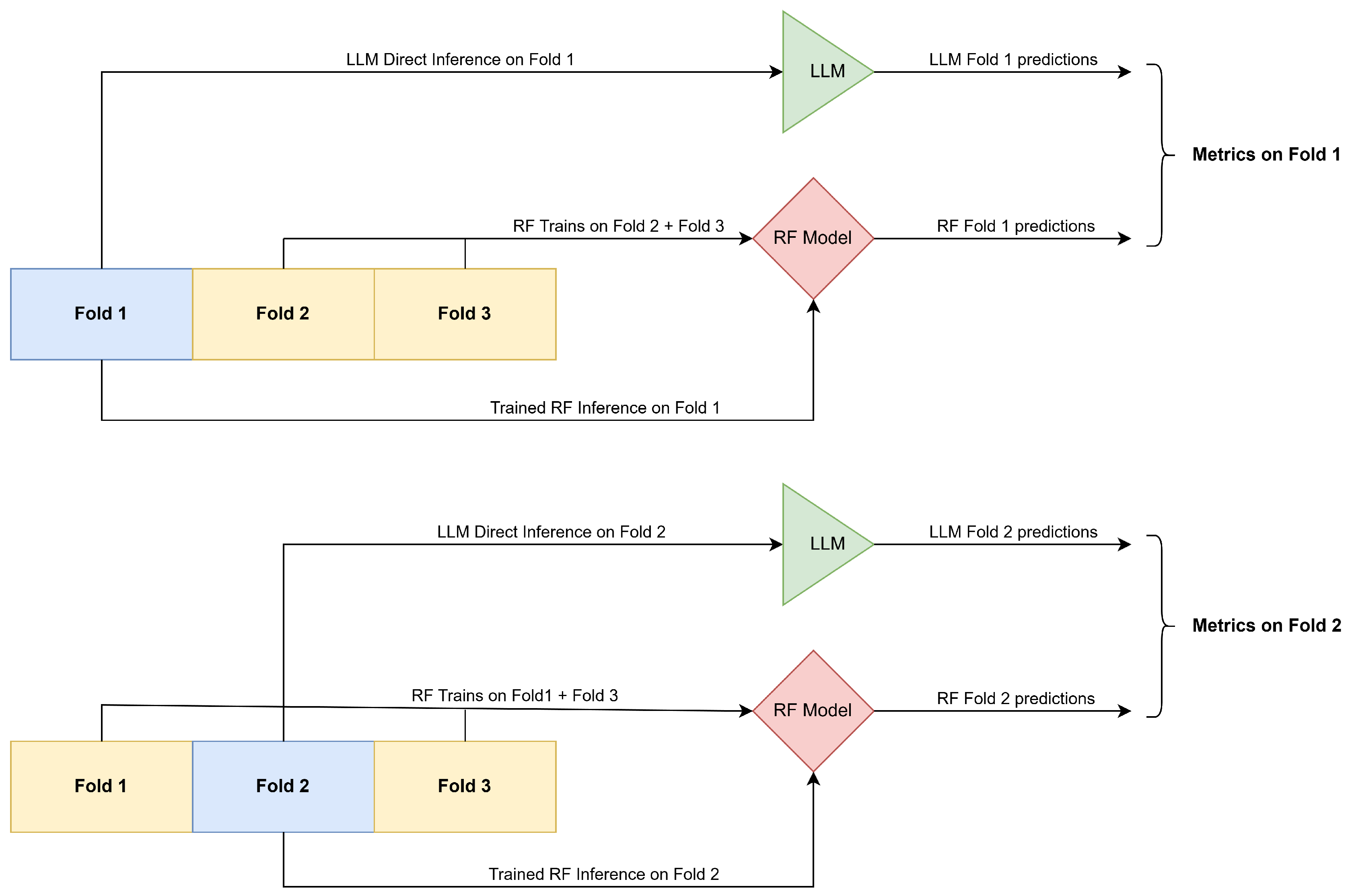
Figure 2.
F1-score same pool comparison: [Gemma 3 12B - RF].
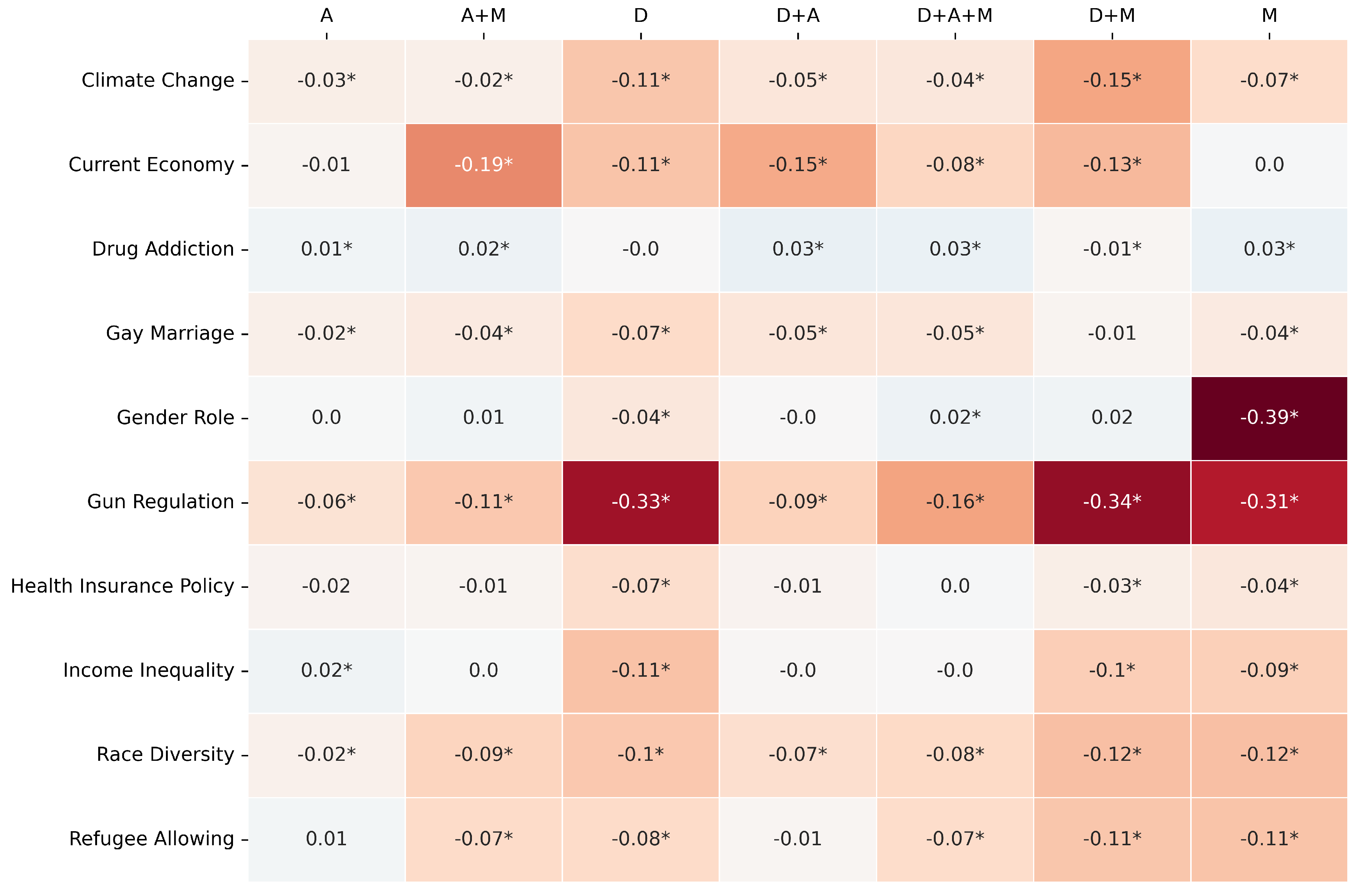
Figure 3.
JS same pool comparison: [RF - Gemma 3 12B].
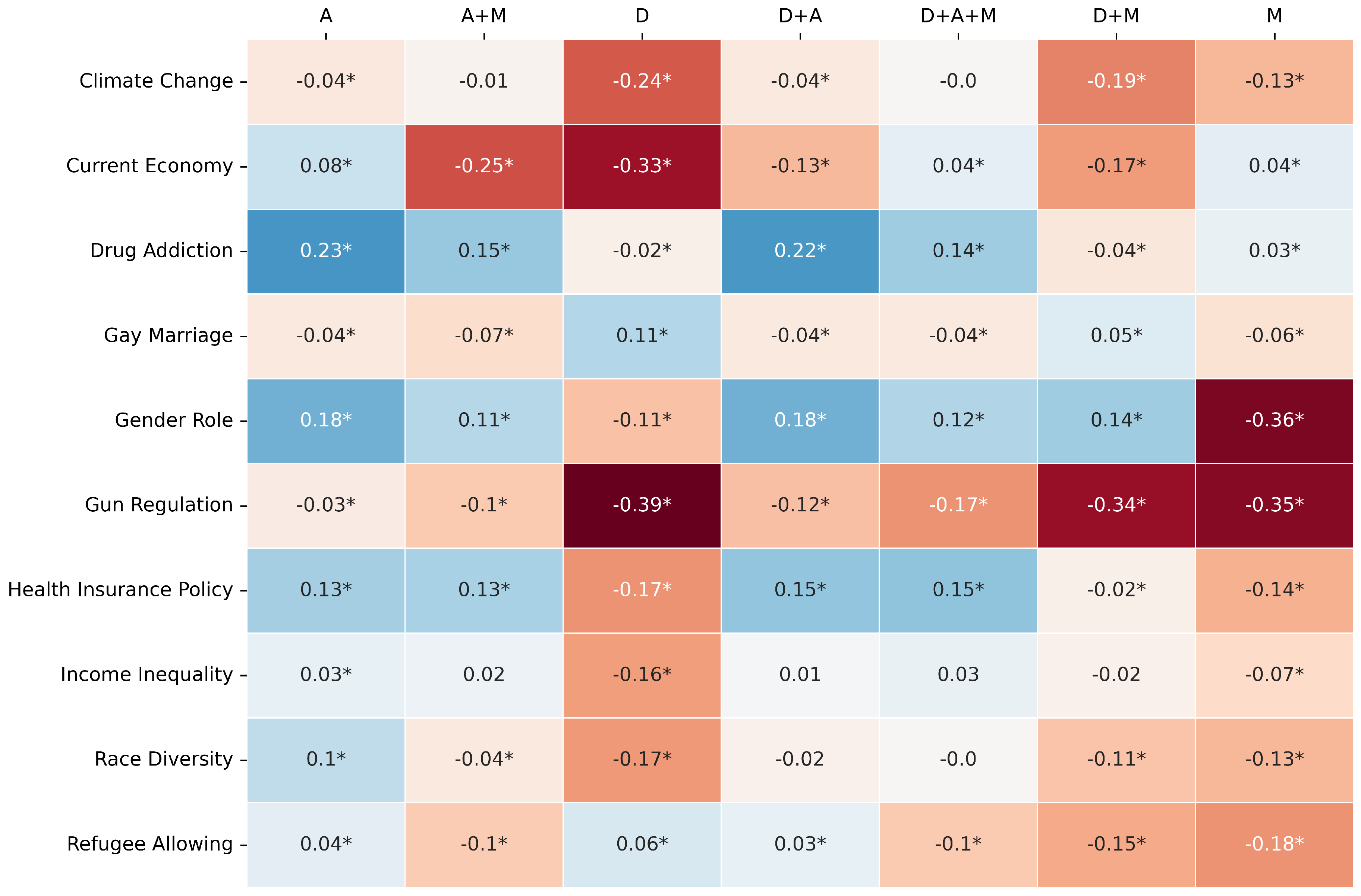
Figure 4.
Cramér’s V same pool comparison: [Gemma 3 12B - RF].
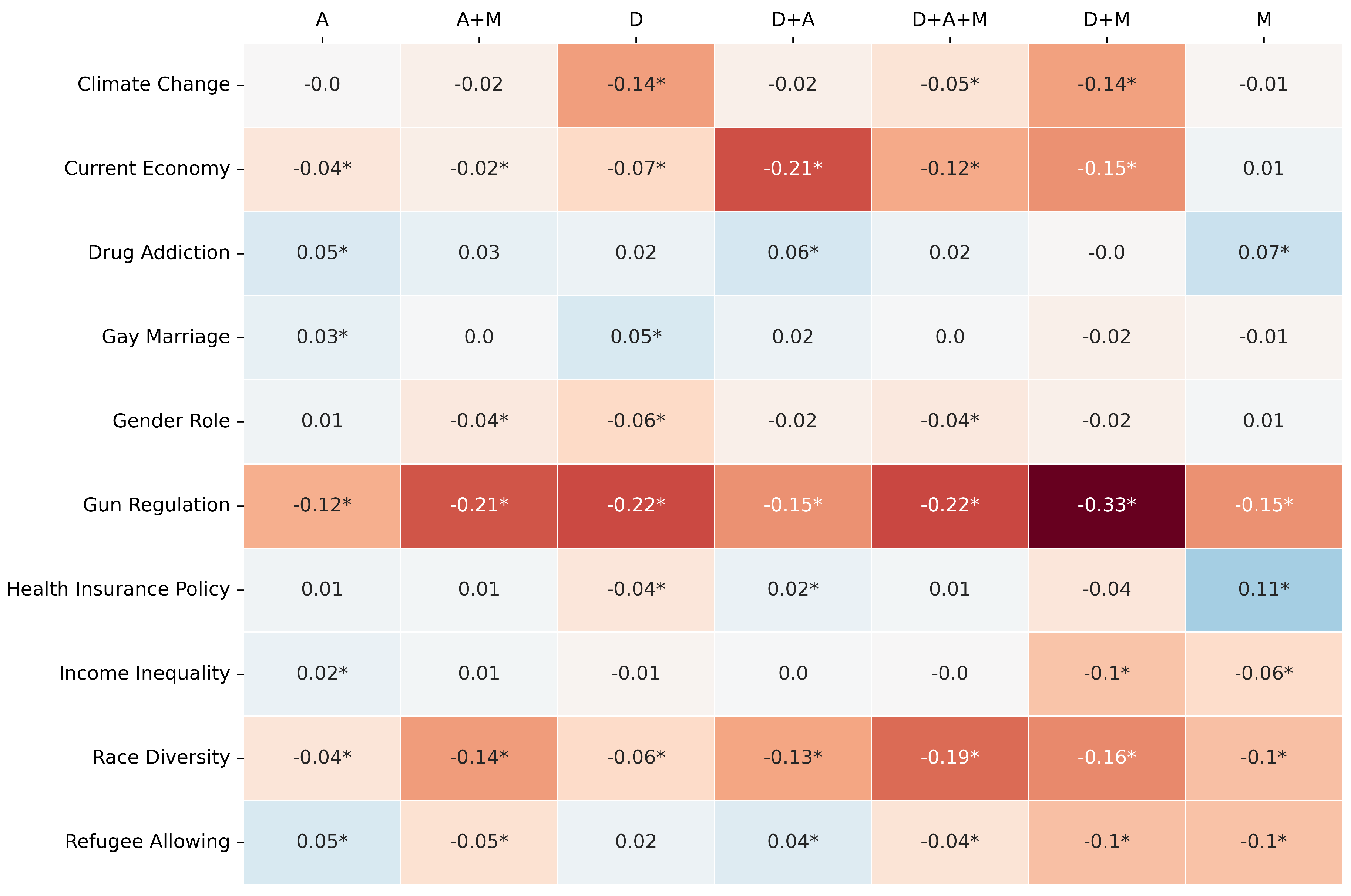
Table 1.
Demographic Backstory Variables
| Variable | Choices |
|---|---|
| Race | 1. White 2. Black 3. Hispanic 4. Asian 5. Native American 6. Mixed |
| Age | [free form value] |
| Gender | 1. Male 2. Female |
| Income (all family) | 1 Under $9,999 2. $10,000-14,999 3. $15,000-19,999 … 15. $80,000-89,999 16. $90,000-99,999 17. $100,000-109,999 … 21. $175,000-249,999 22. $250,000 or more |
| Education | 1. Less than high school credential 2. High school credential 3. Some post-high school, no bachelor’s degree 4. Bachelor’s degree 5. Graduate degree |
| Occupation | 1. For-profit company or organization 2. Non-profit organization 3. Local government 4. State government 5. Military 6. Federal government, as a civilian employee 7. Owner of non-incorporated business 8. Owner of incorporated business 9. for-profit family business |
| City or rural | 1. City person 2. Suburb person 3. Small-town person 4. Country person 5. Neither a city nor rural person |
| Children | 0. No children 1. One child 2. Two children 3. Three children 4. Four or more children |
| Has health insurance | 1. Yes 2. No |
Table 2.
Attitudinal Backstory Variables
| Variable | Choices |
|---|---|
| Ideology | 1. Extremely liberal 2. Liberal 3. Slightly liberal 4. Moderate 5. Slightly conservative 6. Conservative 7. Extremely conservative |
| Party | 1. Strong Democrat 2. Not very strong Democrat 3. Independent who leans Democratic 4. Independent 5. Independent who leans Republican 6. Not very strong Republican 7. Strong Republican |
| Interested in politics | 1. Very interested 2. Somewhat interested 3. Not very interested 4. Not at all interested |
| Trust Media | 1. No 2. A little 3. A moderate amount 4. A lot 5. A great deal |
| Vaccines & Autism | 1. Most scientific evidence shows childhood vaccines cause autism 2. Most scientific evidence shows childhood vaccines do not cause autism |
| Science Experts Necessity | 1. Do not need 2. Need a little 3. Need a moderate amount 4. Need a lot 5. Need a great deal |
| Religion importance | 1. Extremely important 2. Very important 3. Moderately important 4. Little importance 5. Not important at all |
Table 3.
Moral and Social Values Backstory Variables
| Variable | Choices |
|---|---|
| Preferred Child Trait | 1. Obedience 2. Self-reliance 3. Both 4. Neither |
| Death Penalty | 1. Favor 2. Oppose |
| Birthright Citizenship End | 1. Favor a great deal 2. Favor a moderate amount 3. Favor a little 4. Neither favor nor oppose 5. Oppose a little 6. Oppose a moderate amount 7. Oppose a great deal |
| Children Deportation | 1. Favor a great deal 2. Favor a moderate amount 3. Favor a little 4. Oppose a little. 5. Oppose a moderate amount 6. Oppose a great deal |
| Discrimination Women | 1. A great deal 2. A lot 3. A moderate amount 4. A little 5. None |
| Discrimination Black | 1. A great deal 2. A lot 3. A moderate amount 4. A little 5. None |
| Discrimination Gays | 1. A great deal 2. A lot 3. A moderate amount 4. A little 5. None |
| Discrimination Muslins | 1. A great deal 2. A lot 3. A moderate amount 4. A little 5. None |
| Historic Racism Impact | 1. Agree strongly 2. Agree somewhat 3. Neither agree nor disagree 4. Disagree somewhat 5. Disagree strongly |
Table 4.
Survey Topics
| Variable | Question | Choices |
|---|---|---|
| Race diversity | Does the increasing number of people of many different races and ethnic groups in the United States make this country a better place to live, a worse place to live, or does it make no difference? | 1. Better 2. Worse 3. Makes no difference |
| Gender role | Do you think it is better, worse, or makes no difference for the family as a whole if the man works outside the home and the woman takes care of the home and family? | 1. Better 2. Worse 3. Makes no difference |
| Current Economy* | What do you think about the state of the economy these days in the United States? | 1. Good 2. Neither good nor bad 3. Bad |
| Drug addiction | Do you think the federal government should be doing more about the opioid drug addiction issue, should be doing less, or is it currently doing the right amount? | 1. Should be doing more 2. Should be doing less 3. Is doing the right amount |
| Climate change* | How much, if at all, do you think climate change is currently affecting severe weather events or temperature patterns in the United States? | 1. Not at all 2. A little 3. A lot |
| Gay marriage | Which comes closest to your view regarding gay and lesbian couples? | 1. They should be allowed to legally marry 2. They should be allowed to form civil unions but not legally marry 3. There should be no legal recognition of gay or lesbian couples relationship |
| Refugee allowing | Do you favor, oppose, or neither favor nor oppose allowing refugees who are fleeing war, persecution, or natural disasters in other countries to come to live in the U.S.? | 1. Favor 2. Oppose 3. Neither favor nor oppose |
| Health insurance | Do you favor an increase, decrease, or no change in government spending to help people pay for health insurance when people cannot pay for it all themselves? | 1. Increase 2. Decrease 3. No change |
| Gun regulation | Do you think the federal government should make it more difficult for people to buy a gun than it is now, make it easier for people to buy a gun, or keep these rules about the same as they are now? | 1. More difficult 2. Easier 3. Keep these rules about the same |
| Income inequality | Do you favor, oppose, or neither favor nor oppose the government trying to reduce the difference in incomes between the richest and poorest households? | 1. Favor 2. Oppose 3. Neither favor nor oppose |
Table 5.
Performance comparison between Gemma 3 12B and baseline models for Experiment 1. Reported metrics are averaged across folds. Lower Jensen–Shannon distance (JSD) indicates better distributional alignment; higher Cramér’s V and F1-score indicate stronger predictive and associative performance.
| Topic | Model | F1-score | JSD | Cramér’s V |
|---|---|---|---|---|
| Climate Change | Gemma 3 12B | 0.59 | 0.21 | 0.41 |
| Random | 0.36 | 0.29 | 0.04 | |
| Constant | 0.41 | 0.51 | - | |
| Current Economy | Gemma 3 12B | 0.52 | 0.08 | 0.29 |
| Random | 0.35 | 0.11 | 0.04 | |
| Constant | 0.29 | 0.59 | - | |
| Drug Addiction | Gemma 3 12B | 0.56 | 0.20 | 0.10 |
| Random | 0.40 | 0.37 | 0.04 | |
| Constant | 0.58 | 0.41 | - | |
| Gay Marriage | Gemma 3 12B | 0.68 | 0.10 | 0.30 |
| Random | 0.38 | 0.33 | 0.03 | |
| Constant | 0.59 | 0.40 | - | |
| Gender Role | Gemma 3 12B | 0.61 | 0.12 | 0.20 |
| Random | 0.38 | 0.34 | 0.04 | |
| Constant | 0.52 | 0.44 | - | |
| Gun Regulation | Gemma 3 12B | 0.59 | 0.25 | 0.29 |
| Random | 0.38 | 0.30 | 0.03 | |
| Constant | 0.38 | 0.53 | - | |
| Health Insurance Policy | Gemma 3 12B | 0.59 | 0.23 | 0.29 |
| Random | 0.36 | 0.24 | 0.03 | |
| Constant | 0.42 | 0.51 | - | |
| Income Inequality | Gemma 3 12B | 0.61 | 0.06 | 0.40 |
| Random | 0.35 | 0.12 | 0.03 | |
| Constant | 0.32 | 0.57 | - | |
| Race Diversity | Gemma 3 12B | 0.60 | 0.19 | 0.21 |
| Random | 0.37 | 0.32 | 0.03 | |
| Constant | 0.42 | 0.51 | - | |
| Refugee Allowing | Gemma 3 12B | 0.47 | 0.37 | 0.25 |
| Random | 0.36 | 0.22 | 0.03 | |
| Constant | 0.40 | 0.52 | - |
Table 6.
Gemma 3 12B best performance across variable pools in Experiment 2. For each survey topic and metric, the table shows the variable pool that yielded the peak performance, along with the corresponding best F1-score, JSD, and Cramer’s V.
Table 6.
Gemma 3 12B best performance across variable pools in Experiment 2. For each survey topic and metric, the table shows the variable pool that yielded the peak performance, along with the corresponding best F1-score, JSD, and Cramer’s V.
| Topic | F1-score | JS | Cramér’s V | F1-score pool | JS pool | Cramér’s V pool |
|---|---|---|---|---|---|---|
| Climate Change | 0.70 | 0.15 | 0.44 | A+M | A+M | A+M |
| Current Economy | 0.53 | 0.08 | 0.35 | A | A | A+M |
| Drug Addiction | 0.62 | 0.12 | 0.12 | M | A | M |
| Gay Marriage | 0.66 | 0.19 | 0.31 | A | A | A |
| Gender Role | 0.63 | 0.05 | 0.20 | D+A+M | A | D+A |
| Gun Regulation | 0.62 | 0.20 | 0.35 | A | A | D+A |
| Health Insurance Policy | 0.62 | 0.06 | 0.39 | D+A+M | D+A | M |
| Income Inequality | 0.61 | 0.10 | 0.42 | A+M | A | A+M |
| Race Diversity | 0.60 | 0.08 | 0.26 | A | A | D+A |
| Refugee Allowing | 0.57 | 0.11 | 0.30 | A | A | D+A+M |
Table 7.
RF best performance across variable pools in Experiment 2. For each survey topic and metric, the table shows the variable pool that yielded the peak performance, along with the corresponding best F1-score, JSD, and Cramer’s V.
Table 7.
RF best performance across variable pools in Experiment 2. For each survey topic and metric, the table shows the variable pool that yielded the peak performance, along with the corresponding best F1-score, JSD, and Cramer’s V.
| Topic | F1-score | JS | Cramér’s V | F1-score pool | JS pool | Cramér’s V pool |
|---|---|---|---|---|---|---|
| Climate Change | 0.72 | 0.12 | 0.46 | A+M | M | A+M |
| Current Economy | 0.56 | 0.15 | 0.37 | A+M | M | A+M |
| Drug Addiction | 0.59 | 0.30 | 0.06 | A+M | M | D+A+M |
| Gay Marriage | 0.69 | 0.15 | 0.30 | D+A | A | A+M |
| Gender Role | 0.62 | 0.23 | 0.22 | A+M | A | D+A+M |
| Gun Regulation | 0.70 | 0.16 | 0.53 | D+A+M | M | D+A+M |
| Health Insurance Policy | 0.62 | 0.18 | 0.33 | A+M | M | A+M |
| Income Inequality | 0.61 | 0.13 | 0.41 | A+M | A | A+M |
| Race Diversity | 0.65 | 0.15 | 0.43 | D+A+M | M | D+A+M |
| Refugee Allowing | 0.62 | 0.11 | 0.35 | A+M | M | A+M |
Table 8.
Performance gains across variable pools for Experiment 2 when results from Table 6 are compared to the LLM baseline in Experiment 1 (Table 5). Gains are reported as the difference [Experiment 2 - Experiment 1] for F1-score and Cramer’s V and [Experiment 1 - Experiment 2] for JSD, so that positive values/blue shades consistently favor Experiment 2.
| Topic | Gain F1-score | Gain JS | Gain Cramér’s V |
|---|---|---|---|
| Climate Change | 0.11* | 0.07* | 0.03* |
| Current Economy | 0.02* | 0.00 | 0.06* |
| Drug Addiction | 0.06* | 0.09* | 0.02 |
| Gay Marriage | -0.02* | -0.09* | 0.02 |
| Gender Role | 0.02* | 0.07* | -0.00 |
| Gun Regulation | 0.04* | 0.05* | 0.05* |
| Health Insurance Policy | 0.03* | 0.17* | 0.10* |
| Income Inequality | 0.00 | -0.04* | 0.02* |
| Race Diversity | 0.00 | 0.11* | 0.05* |
| Refugee Allowing | 0.09* | 0.26* | 0.05* |
Table 9.
Performance differences across variable pools for Experiment 2 when results from Table 6 are compared to the peak RF performance from Table 7. Differences are calculated as [Peak LLM score - Peak RF score] for F1-score and Cramer’s V, and [Peak RF JSD - Peak LLM JSD] for JSD, so that positive values/blue shades consistently favor the LLM.
| Topic | Diff F1-score | Diff JS | Diff Cramér’s V |
|---|---|---|---|
| Climate Change | -0.02* | -0.02* | -0.02 |
| Current Economy | -0.03* | 0.07* | -0.02* |
| Drug Addiction | 0.02* | 0.18* | 0.06* |
| Gay Marriage | -0.03* | -0.04* | 0.02 |
| Gender Role | 0.01* | 0.18* | -0.03 |
| Gun Regulation | -0.08* | -0.04* | -0.19* |
| Health Insurance Policy | 0.00 | 0.12* | 0.06* |
| Income Inequality | 0.00 | 0.03* | 0.01 |
| Race Diversity | -0.05* | 0.08* | -0.17* |
| Refugee Allowing | -0.06* | -0.00 | -0.04* |
Table 10.
Gemma 3 12B best performance across variable pools in Experiment 3. For each survey topic and metric, the table shows the variable pool that yielded the peak performance, along with the corresponding best F1-score, JSD, and Cramer’s V. Here we instruct the LLM to perform Feature Selection.
| Topic | F1-score | JS | Cramér’s V | F1-score pool | JS pool | Cramér’s V pool |
|---|---|---|---|---|---|---|
| Climate Change | 0.69 | 0.09 | 0.42 | D+A | D+A | D+A+M |
| Current Economy | 0.55 | 0.06 | 0.36 | A+M | A | A |
| Drug Addiction | 0.63 | 0.07 | 0.15 | D+M | D+A | D+M |
| Gay Marriage | 0.66 | 0.16 | 0.31 | D+A+M | A | D+A |
| Gender Role | 0.60 | 0.08 | 0.23 | D+A+M | D+A+M | D+A+M |
| Gun Regulation | 0.63 | 0.18 | 0.36 | D+A | A+M | A |
| Health Insurance Policy | 0.58 | 0.17 | 0.34 | D+M | A+M | D+M |
| Income Inequality | 0.62 | 0.02 | 0.41 | A | A | A |
| Race Diversity | 0.60 | 0.03 | 0.25 | D+A | D+A | D+A |
| Refugee Allowing | 0.56 | 0.14 | 0.29 | D+A | D | D+A |
Table 11.
Comparison of peak LLM performance from Experiment 3 and peak RF performance from Experiment 2. Here we instruct the LLM to perform Feature Selection. The “Diff” columns show the performance difference relative to the best LLM result (from Table 6) for the corresponding topic and metric. Differences are calculated as [Peak LLM score - Peak RF score] for F1-score and Cramer’s V, and [Peak RF JSD - Peak LLM JSD] for JSD, so that positive values/blue shades consistently favor the LLM.
| Topic | Diff F1-score | Diff JS | Diff Cramér’s V |
|---|---|---|---|
| Climate Change | -0.03* | 0.04* | -0.04* |
| Current Economy | -0.01 | 0.08* | -0.01 |
| Drug Addiction | 0.04* | 0.23* | 0.09* |
| Gay Marriage | -0.03* | -0.01 | 0.02 |
| Gender Role | -0.01 | 0.15* | 0.00 |
| Gun Regulation | -0.07* | -0.02 | -0.18* |
| Health Insurance Policy | -0.04* | 0.02 | 0.01 |
| Income Inequality | 0.01 | 0.12* | 0.00 |
| Race Diversity | -0.05* | 0.12* | -0.18* |
| Refugee Allowing | -0.07* | -0.04* | -0.05* |
Disclaimer/Publisher’s Note: The statements, opinions and data contained in all publications are solely those of the individual author(s) and contributor(s) and not of MDPI and/or the editor(s). MDPI and/or the editor(s) disclaim responsibility for any injury to people or property resulting from any ideas, methods, instructions or products referred to in the content. |
© 2025 by the authors. Licensee MDPI, Basel, Switzerland. This article is an open access article distributed under the terms and conditions of the Creative Commons Attribution (CC BY) license (http://creativecommons.org/licenses/by/4.0/).
Copyright: This open access article is published under a Creative Commons CC BY 4.0 license, which permit the free download, distribution, and reuse, provided that the author and preprint are cited in any reuse.


