Submitted:
06 July 2025
Posted:
07 July 2025
Read the latest preprint version here
Abstract
There is a voluminous literature concerning the scope of topological relations that span spaces from R^1 to R^2, Z^2, S^1 and S^2, and T^2. In the case of the *^1 spaces, those relations have been considered both as conceptualizations of both spatial relations and also temporal relations. Missing from that list are the set of digital relations that exist within Z^1, representing discretized time or discretized ordered line segments. Discretized time plays an essential role in timeseries data and in spatio-temporal information systems and geo-foundation models where time is represented in layers of consecutive spatial rasters and/or spatial vector objects colloquially referred to as space-time cubes or spatio-temporal stacks. This paper explores the digital relations that exist in Z^1 interpreted as a regular topological space under the digital Jordan curve as well as a folded-over temporal interpretation of that space for use in spatio-temporal information systems and geo-foundation models. It identifies 34 9-intersection relations in Z^1, 42 9-intersection + margin relations in Z^1, and 74 temporal relations in Z^1, utilizing the 9+-intersection. This workcreates opportunities for better spatio-temporal reasoning capacity within spatio-temporal stacks and more direct interface with intuitive language concepts instrumental for effective utilization of spatial tools.
Keywords:
temporal reasoning
; 9-intersection
; 9+-intersection
; spatio-temporal stack
1. Introduction
In a broad sense, temporal reasoning asserts new relations between events localized in time by facts known about the events themselves [1]. We can think of that in either quantitative terms, such as this event concludes 10 minutes before the next scheduled event at 9 AM or we can think of that in qualitative terms, such as this event happens before that other event. As Naïve Geography opines: topology matters, but metric refines [2]. The same is in theory true in time - our temporal language seems to rely on prepositions in many cases to communicate succinctly about temporal concepts in our day-to-day life, just as topological relations are used as the basis for prepositional phrases [3,4]. Both of these concepts have been critical to the formation of the field of geographic information science, as geography almost necessarily invokes both space and time either implicitly or explicitly [5,6].
Temporal reasoning, however, can be more rigidly classified [1]. Over the decades of research in developing spatial and temporal reasoning, researchers have identified many first-order logic, propositional logic, and reified logic structures for evaluating both spatial and temporal relations. These types of techniques include formalisms such as the Allen interval algebra [7], the 4-intersection [8], the 9-intersection [9], the dimensionally-extended 9-intersection [10], and the region connection calculus [11], amongst others. These types of reasoning structures have become implemented in different software products to answer core questions in modern day applications, but nevertheless, they do not exhaust all possibilities or all aspects of temporal reasoning [1,12] or even spatial reasoning [13]. A basic compendium of qualitative relational sets that have been described in literature is shown in Table 1.
The structure of Table 1 places continuous vector spaces above discretized raster spaces, ranging from continuous to discrete, linear to planar, and planar to spherical. As becomes evident in the bottom four rows of the table, discrete spaces (-spaces and -spaces) lack foundational research into the relationships between line segments in these spaces, with the first column entirely devoid of formalisms that relate these items together. Without these relations, information systems lay devoid of the insights garnered from them, a massive oversight given the saliency of topology toward human reasoning [2,3,4,25]. It is noteworthy that relations would be derivable from relations, just as relations are derivable from relations as the objects have codimension 1 to the space. As such, there is a notable gap in the research literature for and with respect to lines. Temporal objects themselves are almost always conceptualized in one form or another as lines, because we have a distinctive concept of intervals being represented in that way that permeates fields such as data visualization [26].
As data become more and more a lynchpin in an informatics driven world across various disciplines and methods of inquiry, the need to fill the gaps in and are paramount. and are essential for both geographic information systems and Geo-AI [27] in that they represent temporal layering () and rasterized images (). Objects such as roads and streams in rasterized images would necessarily take on this type of format, an overtly spatial concept. Since layering is inherently discrete, is automatically endowed in a vertical sense as a necessity. When layering represents time, temporal relations (important vocabulary for creating descriptions of changes of data) demonstrate the sheer importance of having this space unlocked in the literature, unlocking a plethora of expressive spatio-temporal possibilities. Such an advance would lead to the potential to address human-centric queries in the spatio-temporal stack [28,29], a common data type in modern spatial data science applications which couple spatial raster layers at different timestamps. Unlike where all dimensions have a similar role, the spatio-temporal stack’s vertical dimension has core semantic differences to its lateral ones, which makes it imperative to understand as a simultaneous cross product: , where represents time and represents space. Similarly, we could also intuit a space where the spatial layers of the stack represent vector objects at discretized timestamps. This type of work has already been conducted in an setting [30], but discretized representations have always theoretically lagged behind their continuous counterparts in geographic information science.
When utilizing to represent ordered discrete points in a timeseries, digital line segments represent intervals of time. This could be the hours of a day in which the sun is above the horizon, or the minutes in which an animal is engaging in a single foraging bout or countless other applications. These intervals become the backdrop for countless important questions, either on their own or in conjunction with spatial relations or other restrictive tasks in spatio-temporal relational databases or in geo-foundation models [27].
In this paper, we aim to fill the gap in the literature for intervals in , first as order invariant (representing the sheer spatial relationship within that space) and then as order dependent (representing temporal relations in that space). We accomplish this using the 9-intersection model [9] and then, when moving to temporal relations, the 9+intersection model [31].
The remainder of this paper is structured as follows. Section 2 focuses on the mathematics behind this work, culminating in the 9-intersection family of models. Section 3 details the current state of line-line relations in , both from a temporal [7] and spatial [8,9] perspective. Section 4 focuses on constraints that can be used to generate the discrete linear relations in . Section 5 transforms these relations into their temporal counterparts through folding and extension into the 9+ intersection. Finally, section 6 provide discusses the work and calls for future work in this area.
2. Foundational Mathematics for the Paper
The mathematics of qualitative topological relations in the 9-intersection family of models have their backbone in a hybridized version of point-set and algebraic topology [8,9]. In this section, we detail the foundations of point-set topology [32] that will loosely be translated conceptually into digital lines in .
Definition 1 (Interior):
Let A be a set of points within a topological space X. The interior of A, denoted , is the largest open set from the topological space X contained within A.
Definition 2 (Exterior):
Let A be a set of points within a topological space X. The complement of the set A, denoted by , represents the exterior of the set.
Definition 3 (Closure):
Let A be a set of points within a topological space X. The closure of the set A, denoted , is the smallest closed set from the topological space X, that contains A.
Definition 4 (Boundary):
Let A be a set of points within a topological space X. The boundary of the set A, denoted , is the set .
The interior, boundary, and exterior of an object form the vocabulary for the 9-intersection matrix [9]. The 9-intersection matrix considers the intersection between these topological components of two such objects A and B in a pairwise manner.
This formalism was designed with simple objects in mind and gives binary detail (yes or no) about whether an intersection is empty or not. Simple objects in a naïve sense are those that have connected interiors, boundaries, and exteriors. Other types of embedding spaces and other types of objects create circumstances where an object may separate portions of the interior (or any other part) from one another. In situations such as this, an extension to the 9-intersection matrix called the 9+-intersection matrix [31] was developed. This has been used to describe simple objects [33], raster-based objects [22,34], and directed line segments [31] by deconstructing the topological components into regular prototypical simple objects. That technique has also been used to develop nomenclatures for scene recognition [35,36,37,38]. A different extension of this technique is known as the dimensionally extended 9-intersection matrix [10].
In the case of a digital line in , objects have disconnected exterior components and disconnected boundary components by default, all the while maintaining a connected interior (if the interior exists at all). If the interior does not exist, then the two boundary points are connected, but in no circumstance may the exterior be connected. The boundary points, however, have a distinct characterization in that one of them is specifically the starting point, while the other is the ending point when we consider concepts such as flow, routing, or time. This creates a 5x5 grid to explain topological relations within the 9+-intersection matrix that can be recombined into the 9-intersection as needed [34].
Three types of approaches are used to represent topological objects in not only continuous spaces, but digital spaces as well. The most simplistic utilizes the standard digital topology, resulting in pixels as interior or exterior and the edge between the outermost pixels as the boundary [32,39]. This approach yields for regions in the same set of relations as exist in [21]. The second approach is the digital Jordan curve [40]. Mirroring the philosophy of the point-set topology Jordan curve theorem, the outermost pixels of an object are declared to be its boundary pixels, thus every boundary pixel theoretically borders both interior pixels and exterior pixels, while interior pixels never border exterior pixels and vice versa. This approach yields 16 relations in under the 9-intersection [20], and a further three additional relations when employing the 9+-intersection [31]. The final method for representing these types of regions incorporates a margin approach [41]. The margin approach identifies rings on each side of the boundary to help alert if objects are near each other. This approach adds the additional three relations in [20]. This type of approach has been used to extend beyond non-simple regions to simply connected regions (yielding 62 relations) [23] and has been extended to the digital sphere (yielding 29 relations) [24]. In this paper, we will utilize the digital Jordan curve, though it would be possible to include a margin approach to provide subtle distinctions between various digital Jordan curve relations with minimal modification.
For the remainder of this paper, we will consider the class of intervals represented in (Definition 6). Each interval can be seen as simply a line segment in the space (pursued in Section 4), but also can be seen as a directed line segment with a starting point and an ending point (pursued in Section 5).
Definition 5 (Connected): Let P be a collection of pixels in a discrete space. P is connected if there exists an exhaustive sequence of pixels p1, p2, … pn such that pi neighbors both pi-1 and pi+1.
Definition 6 (Interval object): Let I be a finite group of connected pixels in consisting of at least two pixels. I is defined as an interval object.
With the definition of connected interval objects constructed, the paper can move forward to constructing constraints that must exist on the 9-intersection relation between two such objects.
3. Line-Line Relations in a Continuous Linear Embedding Space
The seminal research motivating line-line relations in linear embeddings is well established and has been the subject of decades of further research.
Allen’s interval algebra [7] considers the relationships between starting and ending points of two objects. The sequence of the points in question define the relation between the intervals. Allen identified 13 plausible sequences for the four points (Figure 1), collapsible into seven groups:
Using the 9-intersection, intervals in can also be studied. If we consider the pictorial representations in Figure 1, we can assess definitively the 9-intersection matrices associated with them. These are shown in Figure 2:
The folding of the Allen intervals reflects the notion that the order in which the objects occur is irrelevant in the spatial domain in that context. If the order were consequential, the 9+-intersection would be used to capture it by distinguishing the start/end points and the pre- and post-exterior.
With knowledge of the state of the art in continuous space, we can now move on to developing similar relations in discretized spaces. Going forward in the manuscript, we will use these simpler relations to group the more numerous discretized relations.
4. Line-Line Relations in a Discretized Linear Embedding Space
To determine the types of relations available within , we have to consider different types of objects that can form digital intervals. This methodologically is a deviation from continuous spaces where the embedding space is dense.
Digital intervals can have interior pixels or not. The number of interior pixels (0, 1, 2, 3+) can have an impact on the types of digital relations available. An interior with zero pixels creates a line consisting entirely of boundary; an interior with one pixel allows for a single boundary component to exhaust the interior; an interior with two pixels can be exhausted by an object with no interior pixels; an interior with 3+ pixels would facilitate the capability of containing a digital line with an interior. We will thus break our consideration down into different groups of objects to extract the relevant qualitative digital relations in the space using a constraint sieve.
A set of basic constraints exist between an object’s topological components and between the interplay of objects’ topological components within a relation. As such, the discussion begins with constraints that exist independent of an object’s interior cardinality. These constraints largely follow constraint logic used in discretized reasoning papers with respect to region relations [20,23,24,34], amended appropriately to account for the separated exterior and boundary of a digital line.
Constraint 1: An interval object I must have an exterior.
Rationale: is a countably infinite space. Since I is finite by construction, there must exist at least one pixel z that does not belong to that object.
C1 passes down to the 9-intersection that at least one member of the row must be non-empty and that at least one member of the column must also be non-empty.
Constraint 2: Two interval objects I and J in a space must have at least one pixel in common between their exteriors.
Rationale: Consider . Since the cardinality of both I and J is finite, then their union has cardinality at most |I| + |J|, which is still finite. By C1, there exists such a pixel exterior to the union, and therefore exterior to both.
C2 passes down to the 9-intersection that no matter what two objects A and B are under consideration in ,
Constraint 3: An interval object I has exactly two boundary pixels.
Rationale: The definition of boundary utilizing the digital Jordan curve dictates that boundary pixels are those pixels which neighbor exterior pixels. Since I has at least two pixels, two of them (namely the outermost two) must touch . In this case, each boundary pixel touches a different connected component of .
C3 passes down to the 9-intersection that the row must have exactly one or two non-empty intersections and that the column must have exactly one or two non-empty intersections, namely:
These could be 1 only if both boundary pixels occupy the same topological component of their relation partner. In all other cases, these will produce 2.
Constraint 4: If the boundaries of interval objects I and J are identical, then their interiors and exteriors must be identical as well.
Rationale: Constraint 4 depends upon the connectivity of the interior and the finite cardinality of the interior. Since has separated components (and only one of them has a finite cardinality), the one with finite cardinality is the interior, and the union of the other two is the exterior as the boundary must surround the interior.
C4 passes down to the 9-intersection:
Depending on whether objects have interiors or not, the missing intersection () will be either empty (no interior) or non-empty (interior exists).
Constraint 5: If both of the boundaries of interval object I are in the interior of another interval object J, then
.
Rationale: Because the boundary pixels surround the connected interior pixels of I and the interior of J is connected by definition, both and cannot exist in that space.
C5 passes down to the 9-intersection that:
Depending on whether or not objects have interiors, the missing intersection () will be either empty (no interior) or non-empty (interior exists).
Such a constraint can be violated in , just as the similar condition can be violated in when considering continuous line relations (Balbiani and Osmani, 2000).
C1 – C5 provide restrictions that exist independent of whether or not the interior of either or both objects exists. To continue forward, we must identify constraints that exist that are unique to objects that must have interiors.
Constraint 6: If the interior or exterior of an interval object I intersects both the interior and exterior of an interval object J, then .
Rationale: The boundary of an object divides the interior from the exterior. For the interior, this is guaranteed because the interior of I must be connected. For the exterior, this is a bit more work. is disconnected within . To demonstrate this, it must be shown that the interior intersection and the exterior intersection can occur on the same side of I. Consider an exposed interior pixel of J. Without loss of generality, assume that the exposed interior pixel is to the left of I’s boundary. This pixel’s left neighbor is either in J’s interior or boundary. If it is in J’s interior, continue left until the boundary is reached, satisfying the constraint. To violate this constraint would require that I had a separated interior, which by construction is a contradiction of the definition of interval object.
C6 passes down to the 9-intersection that:
Constraint 7: If the two boundaries of interval object I are within the interior of interval object J and the exterior of interval object J respectively, then the two boundaries of J must be within the interior and exterior of object I.
Rationale: By construction, interior and exterior pixels of J must be separated by at least one pixel. Since the interior of object I sits between the two boundary pixels of I, it must include the boundary point of J between these two pixels. Since the interior must remain connected, all pixels between that boundary point and I’s interior boundary pixel are interior of J. Consider the next pixel to the left (or right if beyond) of I’s interior boundary pixel. That pixel is either interior of J or boundary of J. Continue until reaching the boundary of J as in Constraint 6, achieving the result.
C7 passes to the 9-intersection matrix that:
Constraint 8: If both interval objects I and J have a boundary pixel in each others’ interior and their exteriors share a common intersection, then the boundaries of I and J cannot intersect.
Rationale: Similar to in constraint 7, a pixel declared as boundary inside the interior of another object has neighbors that are either interior or boundary. If not boundary, traversing further in that direction will encounter boundary that is in the exterior. Therefore, finding the interior boundary of one results in finding the exterior boundary of the other traversing opposite of one’s own interior. When applied to both objects, no construction can produce a boundary-boundary intersection. Given that C2 asserts that there must be common exterior, this is enough to demonstrate the constraint.
C8 passes to the 9-intersection that:
Constraint 9: If both interval objects I and J have a boundary pixel in each other’s exterior and their interiors share a common intersection, then the boundaries of I and J cannot intersect.
Rationale: Constraint 9 is the dual of C8 [43].
C9 passes to the 9-intersection that:
Constraint 10: If both boundaries of an interval object I are within the exterior of object J, then either the entire interior of I is in the exterior of object J or the interior of I is the closure of J, or the interior of I will cross all three components.
Rationale: These three possibilities stem from the placement of the boundary of I relative to J. If I’s boundary pixel is not adjacent to a boundary pixel of J, then an interior pixel of I intersects J’s exterior. If the other boundary pixel of I occurs sequentially before encountering J’s boundary, then we have the first condition. If I’s interior encounter’s J’s boundary, then it must continue until it reaches and passes J’s other boundary to retain both boundary pixels of I in J’s exterior. This is the third condition. The second condition is attained by placing I’s boundary directly adjacent to J’s boundary on both ends of J. The interior then intersects only J’s interior and boundary.
C10 passes the following constraints to the 9-intersection matrix:
The final constraints (C11 and C12) dictate the conditions for the sieve that guarantee that the objects have an interior or not. For various sets of relations; these two constraints can be turned on or off where appropriate
Constraint 11: Interval object A must have an interior
Constraint 12: Interval object B must have an interior
4.1. Two Objects with Interiors (C11 and C12 Active)
Applying these constraints to the class of 9 intersection relations produces 19 viable topological relations with distinct 9 intersection signatures when the objects both have an interior. That is three more than in the simple region-region relations in [20]. The resulting relations are shown in Figure 3. Notably, the line-line relations in have the exact same set of relations as the corresponding region-region relations in .
4.2. Two Objects with No Interiors
The relations between two objects with no interiors are much simpler to construct conceptually, but can also be constructed by substituting constraints C11 and C12 with constraints that no interior intersection can exist. On an intuitive level, this set can be thought of in three distinct forms: 1) the two boundaries are identical, implying that the two exteriors are equal, 2) the two boundaries are entirely distinct, implying a version of disjoint, and 3) one boundary is in common, while the others are different. This is the equivalent of meet or overlap. The three symbols for this are shown in Figure 4.
4.3. One Object with an Interior, One Object Without an Interior
While this result could be considered using a constraint sieve, this case is just as easily accomplished with a visual inspection. We must consider three distinct cases: 1) the object with an interior has only one interior pixel, 2) the object with an interior has exactly two interior pixels, and 3) the object with an interior has three or more pixels. Each class leads to similar relations, but in some cases there are distinct relations that occur. These classes can alternatively be addressed by substituting either C11 or C12 with its juxtaposition.
4.3.1. Common Core
The common core relations between these three cases are ones where the two pixels of the interior-less object do not encounter the interior of the other object. There are four such cases: disjoint (and its converse) and meet (and its converse), as shown in Figure 5.
4.3.2. One Pixel Interior:
The relations with the one pixel interior that are added all are versions of coversTotal and coveredByTotal. The object that has the one pixel interior will always subsume the other. These relations in this form are not shared by the two pixel interior or above, yet there are distinct covers and coveredBy relations that appear in those sets. These relations are shown in Figure 6.
4.3.3. Two Pixel Interior:
The relations with the two pixel interior that are added are versions of covers, coveredBy, insideTotal, and containsTotal. These relations are shown in Figure 7.
4.3.4. 3+ Pixel Interior:
The relations with more than two pixels in their interior in this group of object relations add the potential for a proper contains or inside. These relations are shown in Figure 8.
When combining all of these sets, we determine 34 distinct 9-intersection symbols between two objects A and B in .
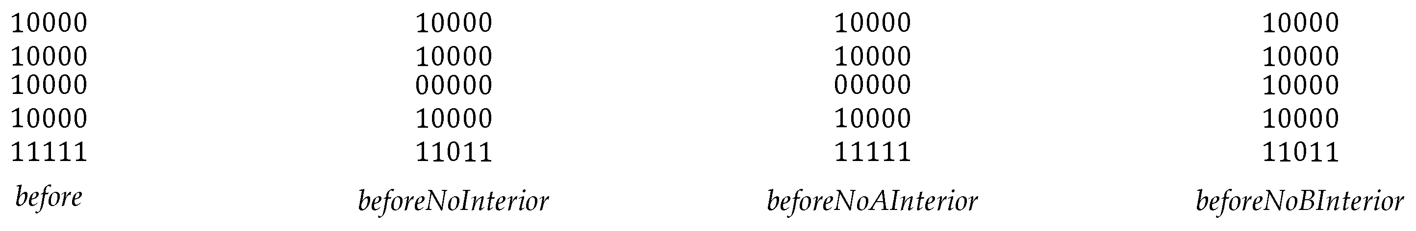
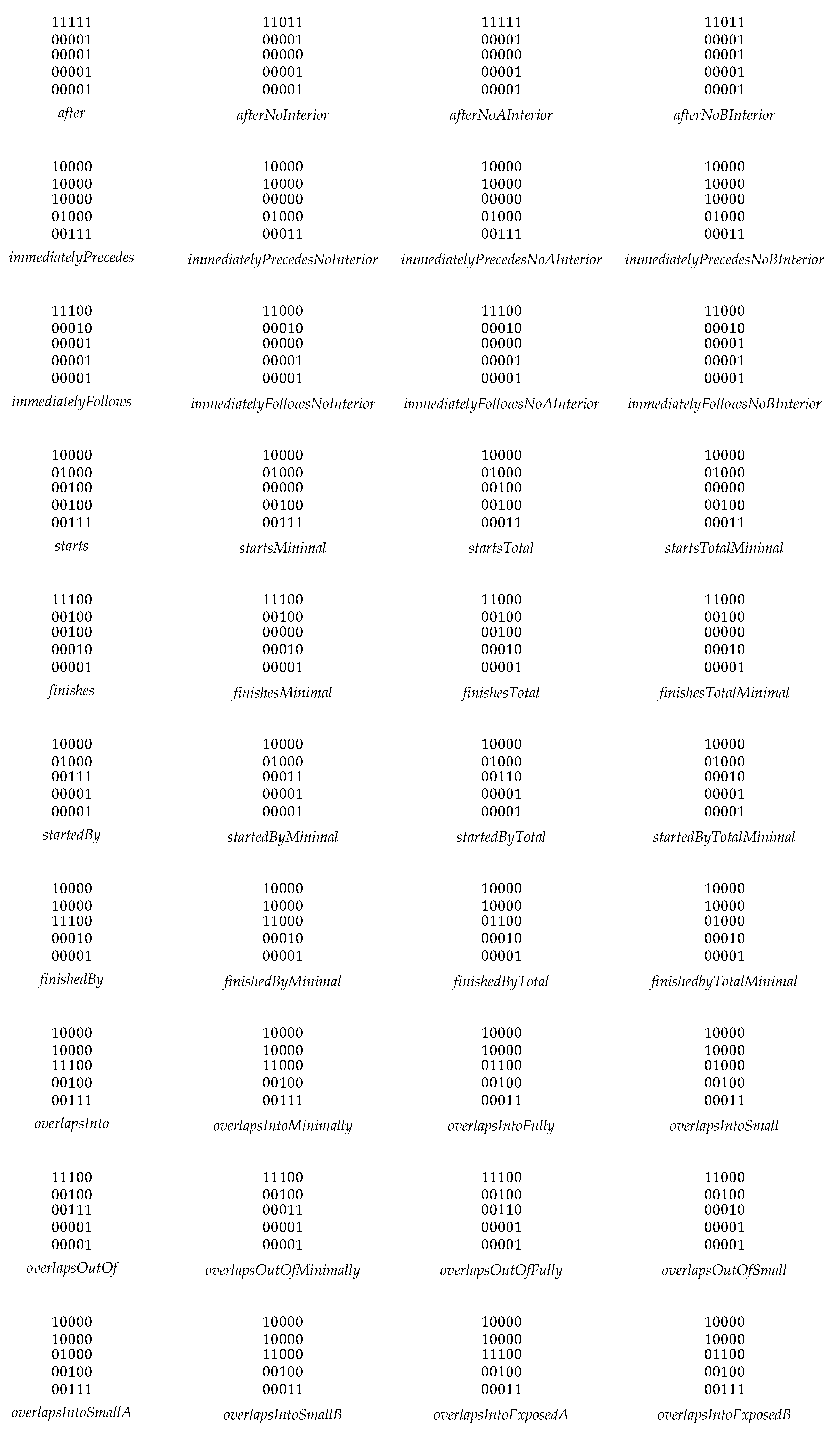
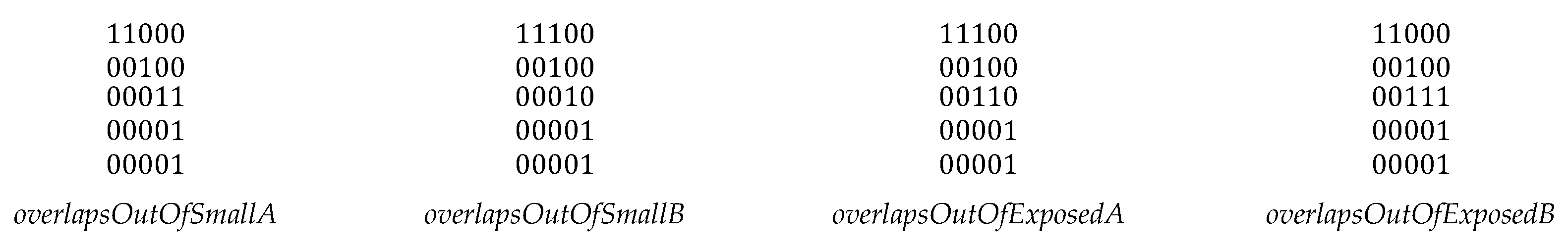
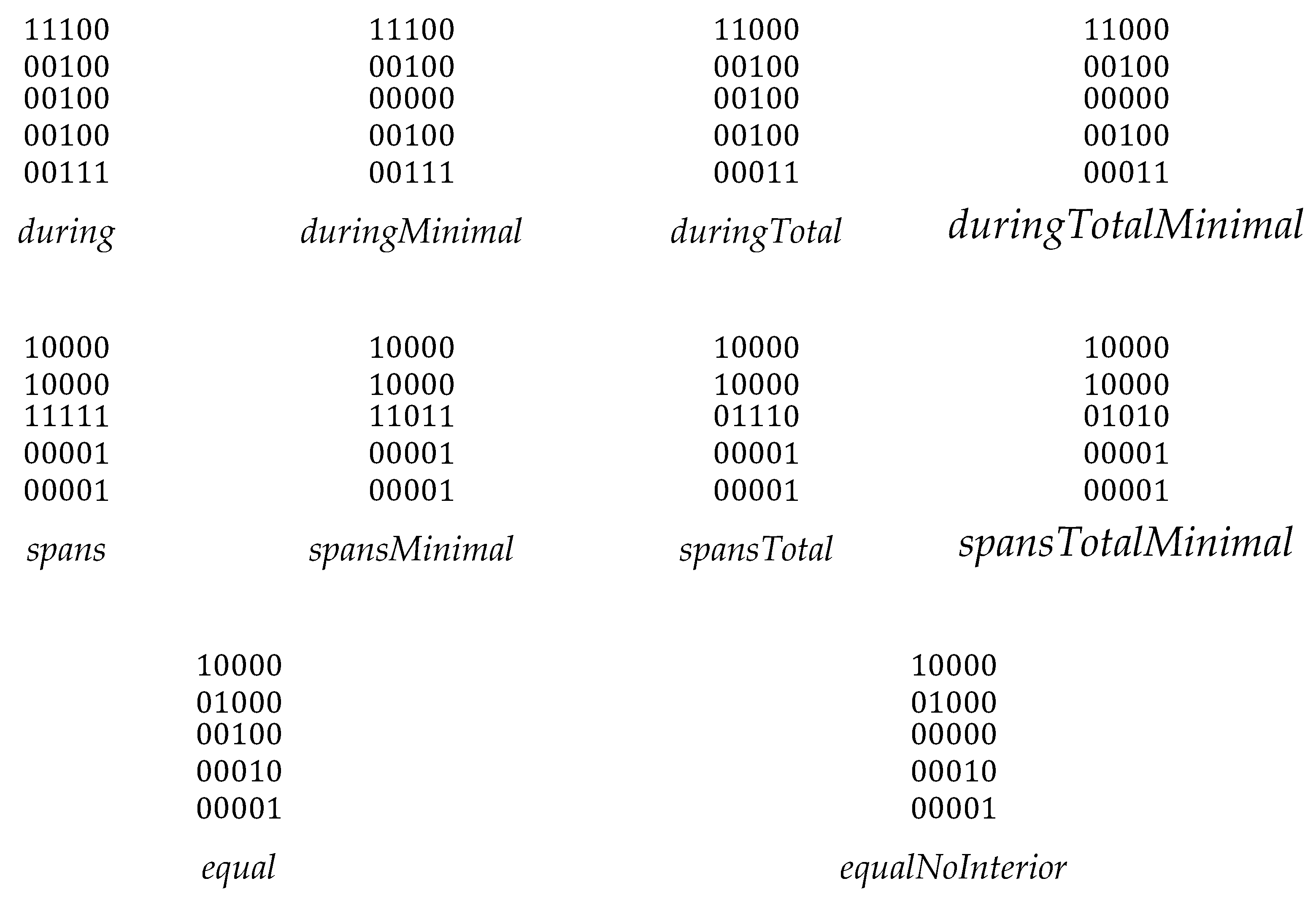
4.4. Visualizing the Set
Figure 9, Figure 10, Figure 11, Figure 12, Figure 13, Figure 14, Figure 15 and Figure 16 demonstrate the various relations as an entire set, organized by their parent line-line relation in . In all cases, the blue object is line A, and the red object is line B. If two boundaries are shared, the boundary point is purple. If the lines encounter common pixels (including boundaries), the two connectors are offset to convey the path (A on bottom, B on top).
This is a good first start, but it is not complete. While most scenarios are accounted for by this simple symmetric exercise, the touch relationships [20,24,34] that are not distinguishable by the 9-intersection for spatial relations disjoint, inside, and contains are not.
The discrete region-region relations in also rely on boundary adjacency (a concept that cannot be modeled directly with the 9-intersection) to produce relations disjointTouch, insideTouch, and containsTouch. Using a similar philosophy, each version of disjoint, pure inside, and pure contains can be bifurcated as in Figure 17. Figure 17 displays the type of relation that is bifurcated from the prototype relation from Figure 9, Figure 11, and Figure 12.
All told, when considering this bifurcation, 42 distinct relations exist between non-ordered lines in . If looking only for distinct 9-intersection matrices, there are 34 relations.
5. Digital Temporal Relations
When is treated as time, this induces an ordering which bifurcates (e.g., the coveredBy relations) into copies depending on which boundary is shared. Temporal relations make use of the 9+-intersection to be able to distinguish which boundary and which exterior they interact with. In a sense, we can accomplish the same concept by examining which types of relations can be formed in two directions, versus relations which are inherently symmetric. The discretized temporal relations will be presented in the 9+-intersection in the following arrangement:
5.1. Bi-Directional Relations from Figures 9, 10, 13, 14, and 16
The following figure constructs the 9+-intersection [31] for each of the bifurcated asymmetric relations found in Figure 9, Figure 10, Figure 13, Figure 14, and Figure 16. The rows of the figure are paired, namely each odd row considers A interacting with B’s before exterior and its start, while the even rows show A interaction with B’s after exterior and its end where applicable.
Figure 18.
Bi-directional Relations in the 9+-Intersection Matrix.
5.2. Symmetric Relations (10), Found in Figures 11, 12, and 15
Figure 19.
Symmetric Relations in the 9+-Intersection.
5.3. Touch Relations (8)
When boundaries become adjacent with the 9+-intersection, interior-exterior intersections are removed. As such, we need to consider the eight relations between objects as shown in Figure 20, producing 16 more temporal relations.
This presents a total of 74 distinct 9+-intersection matrices to represent temporal intervals in . These relations will exchange start and end points of object A as well as the before and after exteriors associated with them.
6. Discussion
In this paper, the relations existing between two continuous sets in were explored, yielding 34 specific digital Jordan curve relations and 42 relations when adding appropriate adjacency information. These sets of relations have core similarities with each other as different objects shift and change size and are all generalizable to similar relations in the set of digital Jordan curve relations in [20]. As the boundaries are disconnected in these types of objects, different types of relations become possible to sustain that are not sustainable in other sets of region-region relations.
These relations were then bifurcated to form corresponding temporal relations, yielding 74 distinct digital Jordan curve relations in an ordered state. These 74 relations become the building blocks for expressing more complex queries in spatio-temporal stacks. This concept recognizes the difference between a pure discrete cube embedding and the corresponding spatio-temporal stack: the vertical dimension is not the same semantically as the horizontal planar ones are.
Digital relations in lead to important unresolved problems in spatio-temporal information science. Most notably, digital relations between lines in have been elusive but represent the missing link in digital spatial reasoning. This paper surrounds that problem with two specific sets of relations that should provide meaningful insights into the process of deriving relationships in that embedding. The biggest challenge to that task is the sequencing of a path. Conceptually speaking, the task of deriving relationships between the pixels should be rather straightforward.
Relations do not exist necessarily in a vacuum, and this particularly true for linear or planar spaces. These spaces in our natural world are often considered in cyclic versions of the same space. To fully realize the potential of spatial and temporal information, it is important to generalize from linear spaces to cyclic spaces. Such adaptations have journeyed from the Allen intervals algebra to the cycle algebra [7,17], the RCC-8 relations journeying to the RCC-11 relations [11,19], the journey from the point-set topological relations to the spherical topological relations [9,18], and the journey from the raster relations in to the raster relations in [20,24]. This set of relations can be transformed using similar processes.
The other important step to take from this starting point is to consider the alphabet of spatio-temporal queries. Research has focused on spatial queries and temporal queries, but the queries that engage both together are fewer in number. Jiang et al. [44] studied the notion of topological changes of objects. While this is an important step, it does not solve issues that involve the sequence of binary relationships more related to conceptual neighborhood graphs [45,46]. That innovation will unlock many doors in spatial informatics in numerous application spaces, most notably as complex spatial phenomena related to species migration and shifting climates are knocking at our doors.
Funding
This research was funded by the National Science Foundation (US), grant number 2019470 and the APC was funded by MDPI.
Conflicts of Interest
The author declares no conflicts of interest.
References
- Goertzel, B.; Geisweiller, N.; Coelho, L.; Janičić, P.; Pennachin, C. Real-World Reasoning: Toward Scalable, Uncertain Spatiotemporal, Contextual and Causal Inference; Atlantic Press: Amsterdam, Netherlands, 2011; pp. 79-97.
- Egenhofer, M.J.; Mark, D.M. Naïve geography. In International Conference on Spatial Information Theory; Frank, A.U., Kuhn, W., Eds.; Springer: Berlin, Germany, 1995; pp. 1-15.
- Dube, M.P.; Egenhofer, M.J. An ordering of convex topological relations. In International Conference on Geographic Information Science; Xiao, N., Kwan, M., Goodchild, M.F., Shekhar, S., Eds. Springer: Berlin, Germany, 2012; pp. 72-86.
- Klippel, A.; Li, R.; Yang, J.; Hardisty, F; Xu, S. In Cognitive and Linguistic Aspects of Geographic Space; Raubal, M., Mark, D.M., Frank, A.U., Eds.; Springer: Berlin, Germany, 2013; pp. 195-215.
- Pred, A. The choreography of existence: comments on Hagerstrand’s time-geography and its usefulness. Economic Geography 1978 53, 207-221. [CrossRef]
- Claramunt, C.; Dube, M.P. A brief review of the evolution of GIScience since the NCGIA Research Agenda initiatives. Journal of Spatial Information Science 2023, 26, 137-150. [CrossRef]
- Allen, J.F. Maintaining knowledge about temporal intervals. Communications of the ACM 1983, 26(11), 832-843. [CrossRef]
- Egenhofer, M.J.; Franzosa, R.D. Point-set topological spatial relations. International Journal of Geographical Information Systems 1991, 5(2), 161-174.
- Egenhofer, M.J.; Herring, J.R. Categorizing binary topological relations between regions, lines, and points in geographic databases. NCGIA Technical Report, 1990.
- Clementini, E.; diFelice, P. A model for representing topological relationships between complex geometric features in spatial databases. Information Sciences 1996, 90(1-4), 121-136. [CrossRef]
- Randell, D.A.; Cui, Z.; Cohn, A.G. A spatial logic based on regions and connection. In Principles of Knowledge Representation and Reasoning; Nebel, B., Rich, C., Swartout, W., Eds.; Morgan Kauffman: San Mateo, United States, 1992; pp. 165-176.
- Pratt, I.; Francez, N. Temporal prepositions and temporal generalized quantifiers. Linguistics and Philosophy 2001, 24(2), 187-222. [CrossRef]
- Dube, M.P.; Hall, B.P. Conceptual neighborhood graphs: event detectors, data relevancy, and language translation. Geography According to ChatGPT 2025 (under revision).
- Egenhofer, M.J.; Definitions of line-line relations for geographic databases. IEEE Data Engineering Bulletin 1993, 16(3), 40-45.
- Reis, R.M.; Egenhofer, M.J.; Matos, J.L. Conceptual neighborhoods of topological relations between lines. In Headway in Spatial Data Handling; Ruas, A., Gold, C., Eds. Springer: Berlin, Germany, 2008; pp. 557-574.
- Egenhofer, M.J.; Mark, D.M. Modelling conceptual neighbourhoods of topological line-region relations. International Journal of Geographical Information Systems 1995, 9(5), 555-565. [CrossRef]
- Balbiani, P.; Osmani, A. A model for reasoning about topologic relations between cyclic intervals. In Principles of Knowledge Representation and Reasoning; Cohn, A.G., Giunchiglia, F., Selman, B., Eds. Morgan Kaufman: San Mateo, United States, 2000; pp. 378-385.
- Egenhofer, M.J. Spherical topological relations. Journal on Data Semantics III 2005, 1, 25-49.
- Li, S.; Li., Y. On the complemented disk algebra. The Journal of Logic and Algebraic Programming 2006, 66(2), 195-211.
- Egenhofer, M.J.; Sharma, J. Topological relations between in regions in ℝ2 and ℤ2. In International Symposium on Spatial Databases; Abel, D.J., Ooi, B.C., Eds. Springer-Verlag: Berlin, Germany, 1993; pp. 316-336.
- Winter, S. Topological relations between discrete regions. In International Symposium on Spatial Databases; Egenhofer, M.J., Herring, J.R., Eds. Springer-Verlag: Berlin, Germany, 1995; pp. 310-327.
- Dube, M.P.; Barrett, J.V.; Egenhofer, M.J. From metric to topology: determining relations in discrete space. In International Conference on Spatial Information Theory; Fabrikant, S., Raubal, M., Bertolotto, M., Davies, C., Freundschuh, S., Eds. Springer: Cham, Switzerland, 2015; pp. 151-171.
- Dube, M.P.; Egenhofer, M.J.; Barrett, J.V.; Simpson, N.J. Beyond the digital Jordan curve: unconstrained simple pixel-based raster relations. Journal of Computer Languages 2019, 54, 100906. [CrossRef]
- Dube, M.P.; Egenhofer, M.J. Binary topological relations on the digital sphere. International Journal of Approximate Reasoning 2020, 116, 62-84.
- Clementini, E.; Sharma, J.; Egenhofer, M.J. Modelling topological spatial relations: strategies for query processing. Computers and Graphics 1994, 18(6), 815-822. [CrossRef]
- Schwabish, J. Better Data Visualizations; Columbia University Press: New York, United States, 2021.
- Xie, Y.; Wang, Z.; Mai, G.; Li, Y.; Jia, X.; Gao, S.; Wang, S. Geo-foundation models: reality, gaps, and opportunities. In Proceedings of the 31st ACM SIGSPATIAL International Conference on Advances in Geographic Information Systems; Damiani, M.L., Renz, M., Eldawy, A., Kroger, P., Nascimento, M.A., Eds. ACM Press, Washington, United States, 2023; pp. 1-4.
- Yuan, M. Use of a three-domain representation to enhance GIS support for complex spatiotemporal queries. Transactions in GIS 1999, 3(2), 137-159. [CrossRef]
- Shen, J.; Chen, M.; Liu, X. Classification of topological relations between spatial objects in two-dimensional space within the dimensionally extended 9-intersection model. Transactions in GIS 2018, 22(2), 514-541. [CrossRef]
- Claramunt, C.; Jiang, B. An integrated representation of spatial and temporal relationships between evolving regions. Journal of Geographical Systems 2001, 3(4), 411-428. [CrossRef]
- Kurata, Y. The 9+-intersection: a universal framework for modeling topological relations. In International Conference on Geographic Information Science; Cova, T.J., Miller, H.J., Beard, M.K., Frank, A.U., Goodchild, M.F., Eds. Springer: Berlin, Germany, 2008; pp. 181-198.
- Adams, C.A.; Franzosa, R.D. Introduction to Topology: Pure and Applied; Pearson Prentice-Hall: Upper Saddle River, NJ, United States, 2008.
- Kurata, Y. 9+-intersection calculi for spatial reasoning on the topological relations between heterogeneous objects. In Proceedings of the 18th SIGSPATIAL International Conference on Advances in Geographic Information Systems; Agrawal, D., Zhang, P., El Abbadi, A., Mokbel, M., Eds. ACM Press: Washington, United States, 2010; pp. 390-393.
- Hall, B.P.; Dube, M.P. Conceptual neighborhood graphs of topological relations in ℤ2. International Journal of Geo-information 2025, 14(4), 150.
- Dube, M.P.; Egenhofer, M.J.; Lewis, J.A.; Stephen, S.; Plummer, M.A. Swiss canton regions: a model for complex objects in geographic partitions. In International Conference on Spatial Information Theory; Fabrikant, S., Raubal, M., Bertolotto, M., Davies, C., Freundschuh, S., Eds. Springer: Cham, Switzerland, 2015; pp. 309-330.
- Lewis, J.A.; Dube, M.P.; Egenhofer, M.J. The topology of spatial scenes in ℝ2. In International Conference on Spatial Information Theory; Tenbrink, T., Stell, J., Galton, A., Wood, Z., Eds. Springer: Cham, Switzerland, 2013; pp. 495-515.
- Lewis, J.A.; Egenhofer, M.J. Oriented regions for linearly conceptualized features. In International Conference on Geographic Information Science; Duckham, M., Stewart, K., Pebesma, E., Eds. Springer: Cham, Switzerland, 2014; pp 333-348.
- Lewis, J.A. A qualitative representation of spatial scenes in ℝ2 with regions and lines. Doctoral Dissertation, University of Maine, Orono, ME, United States, 2019.
- Rosenfeld, A. Digital topology. The American Mathematical Monthly 1979, 86(8), 621-630.
- Vince, A.; Little, C.H. Discrete Jordan curve theorems. Journal of Combinatorial Theory, Series B, 1989, 47(3), 251-261.
- Galton, A. Modes of overlap. Journal of Visual Languages and Computing, 1998, 9(1), 61-79.
- Mate, S.; Burkle, T.; Kapsner, L.A.; Toddenroth, D.; Kampf, M.O.; Sedlmayr, M.; Castellanos, I.; Prokosch, H.U.; Kraus, S. A method for the graphical modeling of relative temporal constraints. Journal of Biomedical Informatics, 2019, 100, 103314. [CrossRef]
- Duntsch, I.; Orlowska, E. Discrete duality for rough relation algebras. Fundamenta Informaticae, 2013, 127(1-4), 35-47. [CrossRef]
- Jiang, J.; Worboys, M.F.; Nittel, S. Qualitative change detection using sensor networks based on connectivity information. Geoinformatica, 2011, 15(2), 305-328. [CrossRef]
- Freksa, C. Temporal reasoning based on semi-intervals. Artificial Intelligence, 1992, 54(1-2), 199-227. [CrossRef]
- Egenhofer, M.J. The family of conceptual neighborhood graphs for region-region relations. In International Conference on Geographic Information Science; Fabrikant, S.I., Reichenbacher, T., van Kreveld, M.J., Schlieder, C., Eds. Springer: Berlin, Germany, 2010; pp. 42-55.
Figure 1.
Allen Interval Algebra, expressed through relations between endpoints [42].
Figure 1.
Allen Interval Algebra, expressed through relations between endpoints [42].
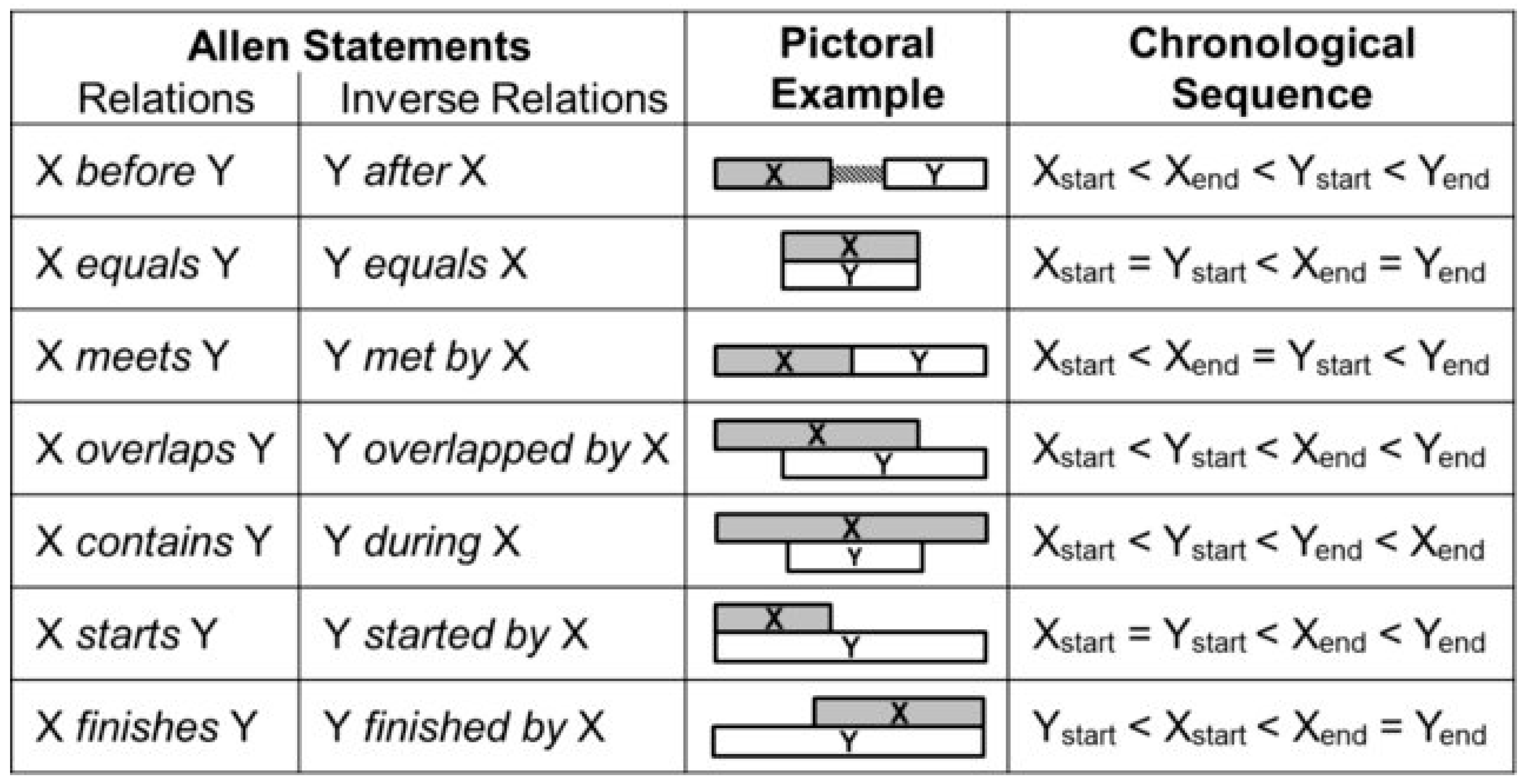
Figure 2.
Line-line relations in : a) before/after, b) equal, c) meets/metBy, d) overlaps/overlappedBy, e) contains, f) during, g) starts/finishes, and h) startedBy/finishedBy.
Figure 2.
Line-line relations in : a) before/after, b) equal, c) meets/metBy, d) overlaps/overlappedBy, e) contains, f) during, g) starts/finishes, and h) startedBy/finishedBy.
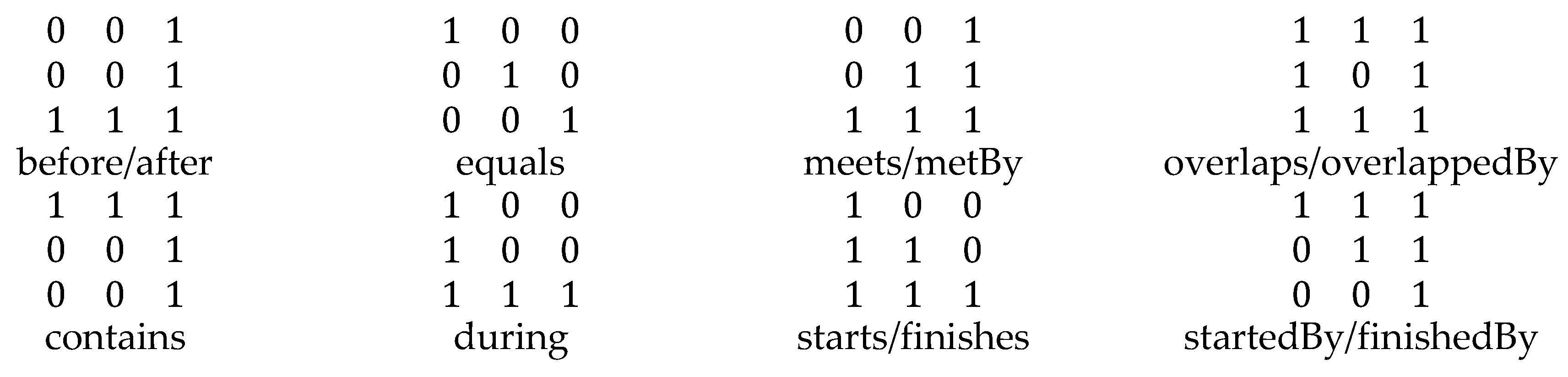
Figure 3.
19 topological relations with distinct 9-intersections that satisfy the constraint sieve described above.
Figure 3.
19 topological relations with distinct 9-intersections that satisfy the constraint sieve described above.
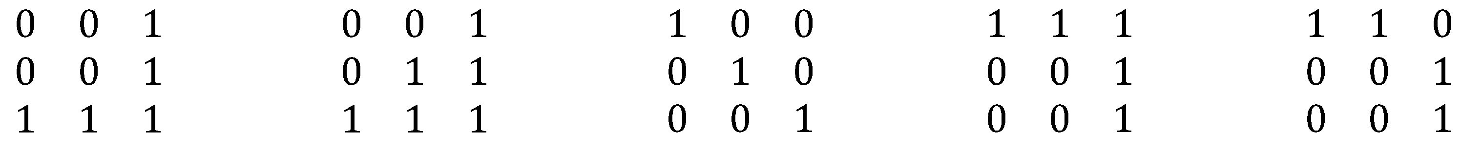
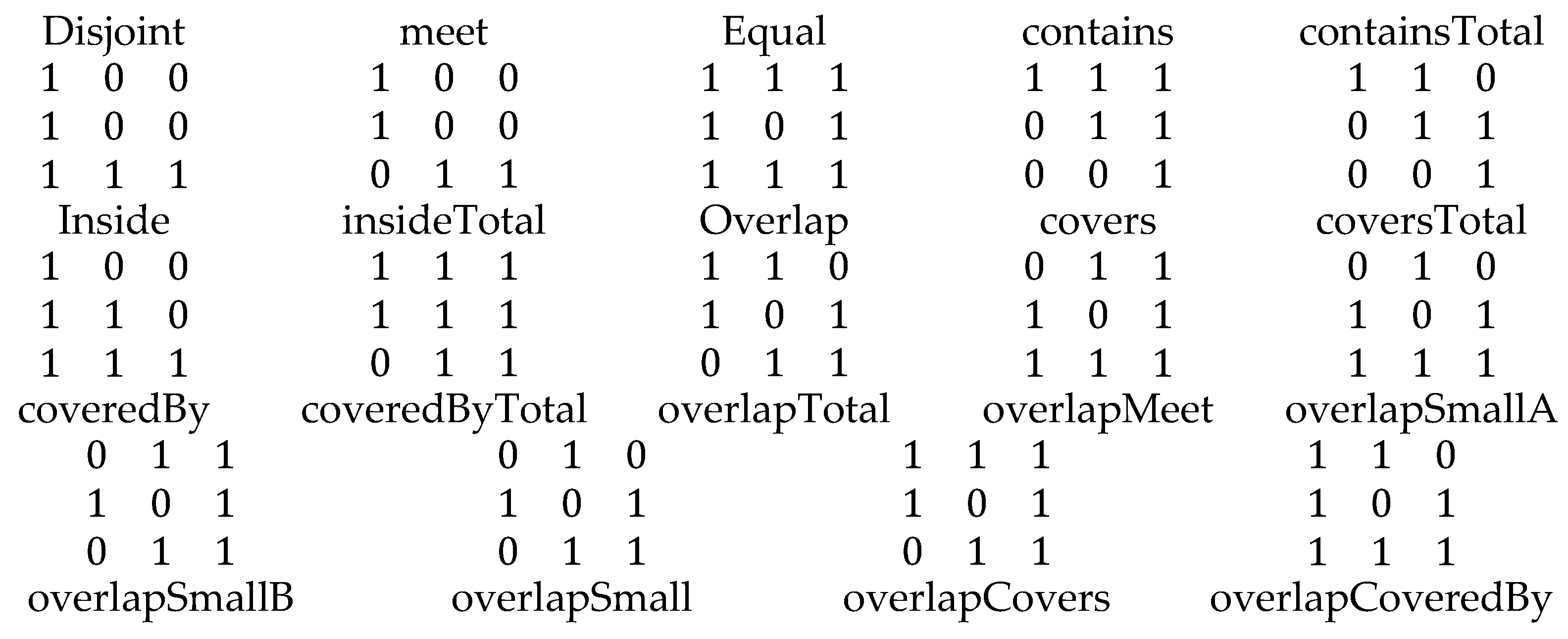
Figure 4.
Three 9-intersection relations resulting from each object having no interior.
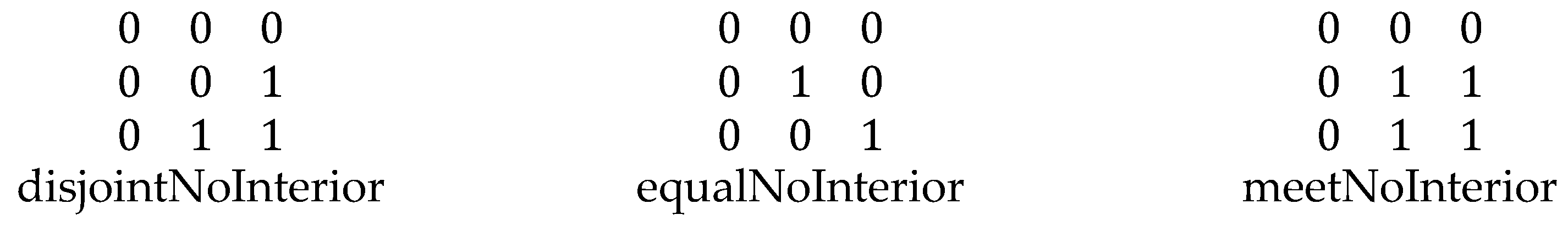
Figure 5.
disjoint and meet relations with one object having no interior.
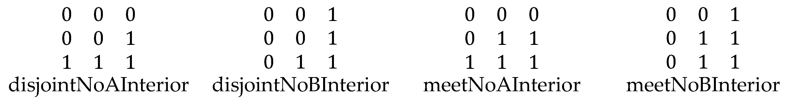
Figure 6.
coveredByTotal and coversTotal relations with one object having no interior and the other having a one pixel interior.
Figure 6.
coveredByTotal and coversTotal relations with one object having no interior and the other having a one pixel interior.
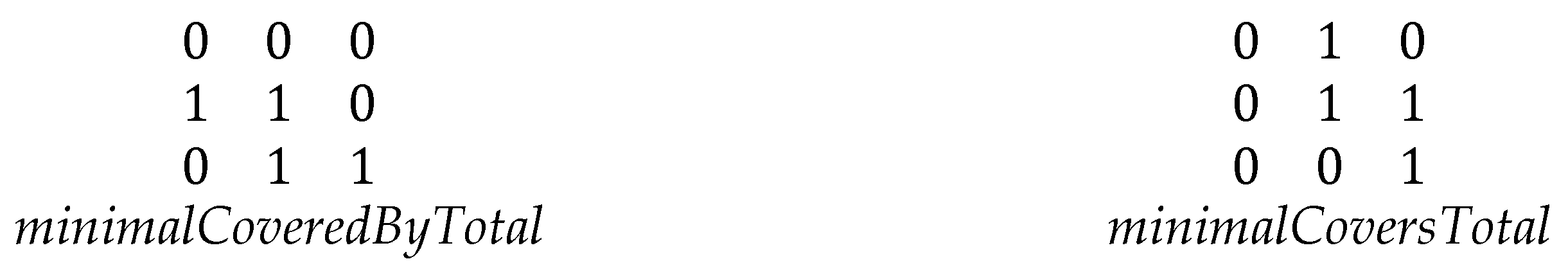
Figure 7.
coveredBy, insideTotal, covers, and containsTotal relations with one object having no interior and the other having a two pixel interior.
Figure 7.
coveredBy, insideTotal, covers, and containsTotal relations with one object having no interior and the other having a two pixel interior.

Figure 8.
contains and inside relations with one object having no interior and the other having a 3+ pixel interior.
Figure 8.
contains and inside relations with one object having no interior and the other having a 3+ pixel interior.
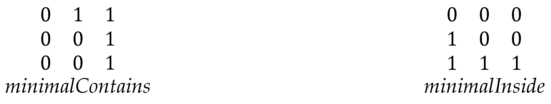
Figure 9.
The four disjoint relations (top to bottom): disjoint, disjointNoAInterior, disjointNoBInterior, and disjointNoInterior.
Figure 9.
The four disjoint relations (top to bottom): disjoint, disjointNoAInterior, disjointNoBInterior, and disjointNoInterior.
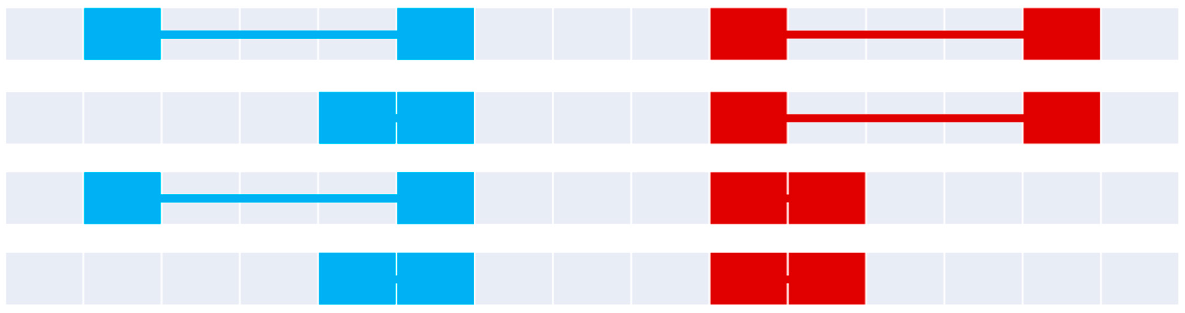
Figure 10.
The four meet relations (top to bottom): meet, meetNoAInterior, meetNoBInterior, and meetNoInterior.
Figure 10.
The four meet relations (top to bottom): meet, meetNoAInterior, meetNoBInterior, and meetNoInterior.

Figure 11.
The four inside relations (top to bottom): inside, minimalInside, insideTotal, and minimalInsideTotal.
Figure 11.
The four inside relations (top to bottom): inside, minimalInside, insideTotal, and minimalInsideTotal.

Figure 12.
The four contains relations (top to bottom): contains, minimalContains, containsTotal, and minimalContainsTotal.
Figure 12.
The four contains relations (top to bottom): contains, minimalContains, containsTotal, and minimalContainsTotal.
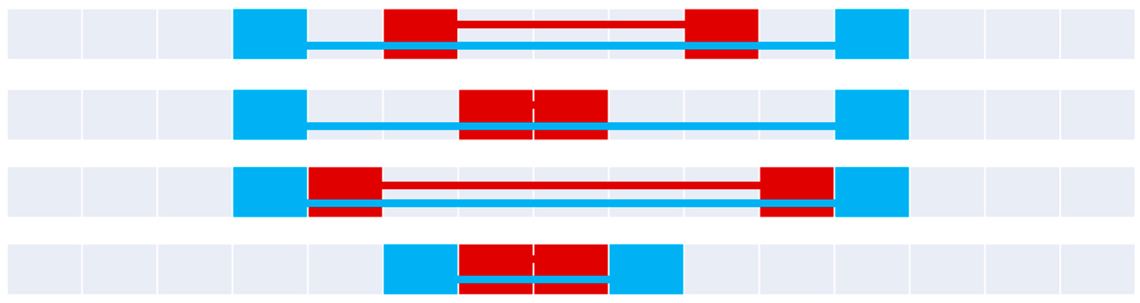
Figure 13.
The four coveredBy relations (top to bottom): coveredBy, minimalCoveredBy, coveredByTotal, and minimalCoveredByTotal.
Figure 13.
The four coveredBy relations (top to bottom): coveredBy, minimalCoveredBy, coveredByTotal, and minimalCoveredByTotal.
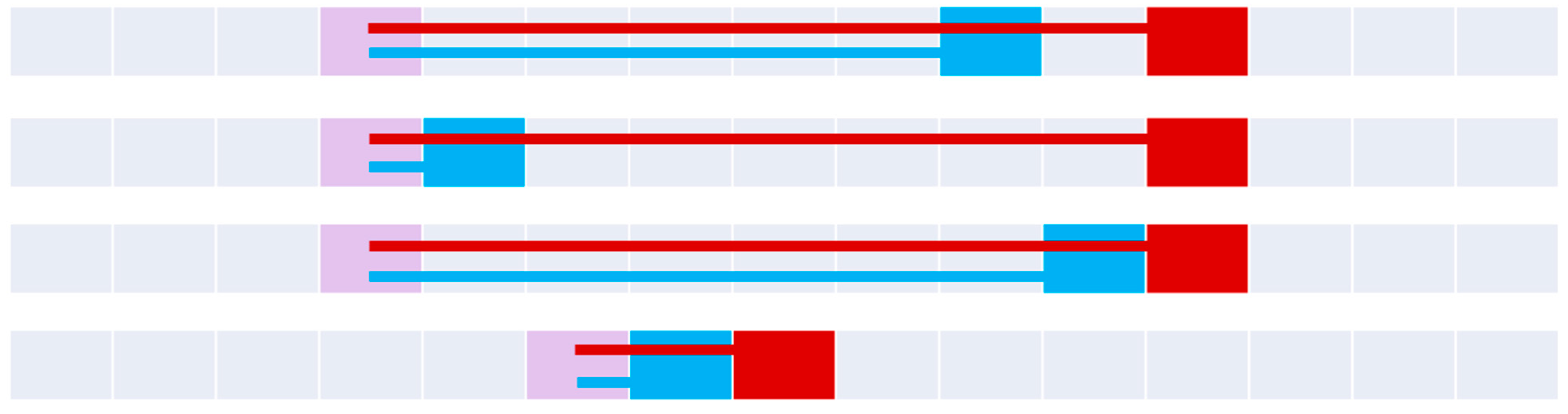
Figure 14.
The four covers relations (top to bottom): covers, minimalCovers, coversTotal, and minimalCoversTotal.
Figure 14.
The four covers relations (top to bottom): covers, minimalCovers, coversTotal, and minimalCoversTotal.
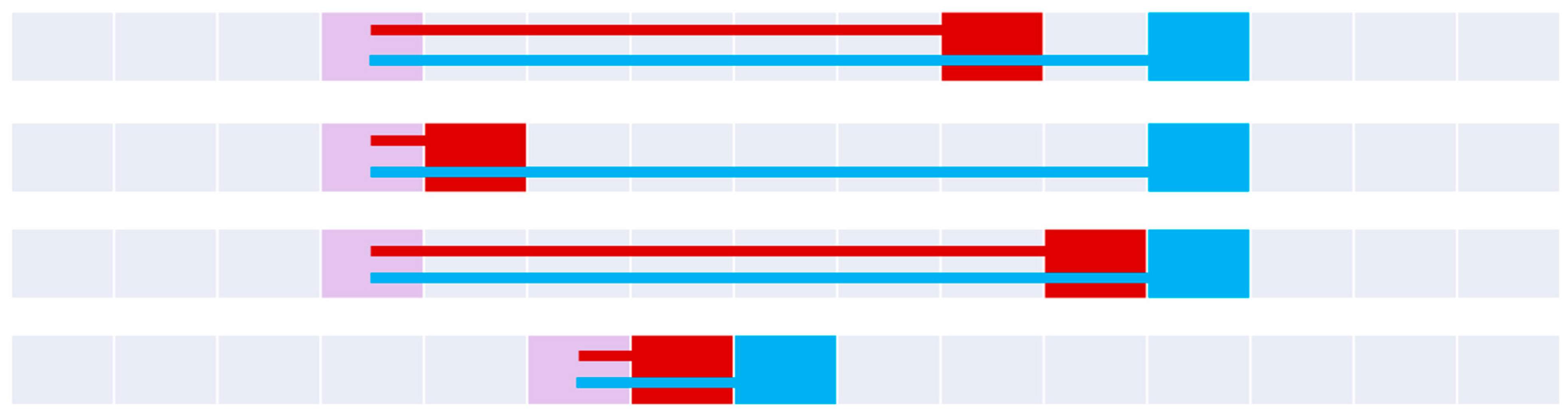
Figure 15.
The two equals relations (top to bottom): equals and equalsNoInterior.

Figure 16.
The eight overlap relations (top to bottom): overlap, overlapTotal, overlapExposedB, overlapExposedA, overlapSmallB, overlapSmallB, overlapMinimally,and overlapSmall.
Figure 16.
The eight overlap relations (top to bottom): overlap, overlapTotal, overlapExposedB, overlapExposedA, overlapSmallB, overlapSmallB, overlapMinimally,and overlapSmall.
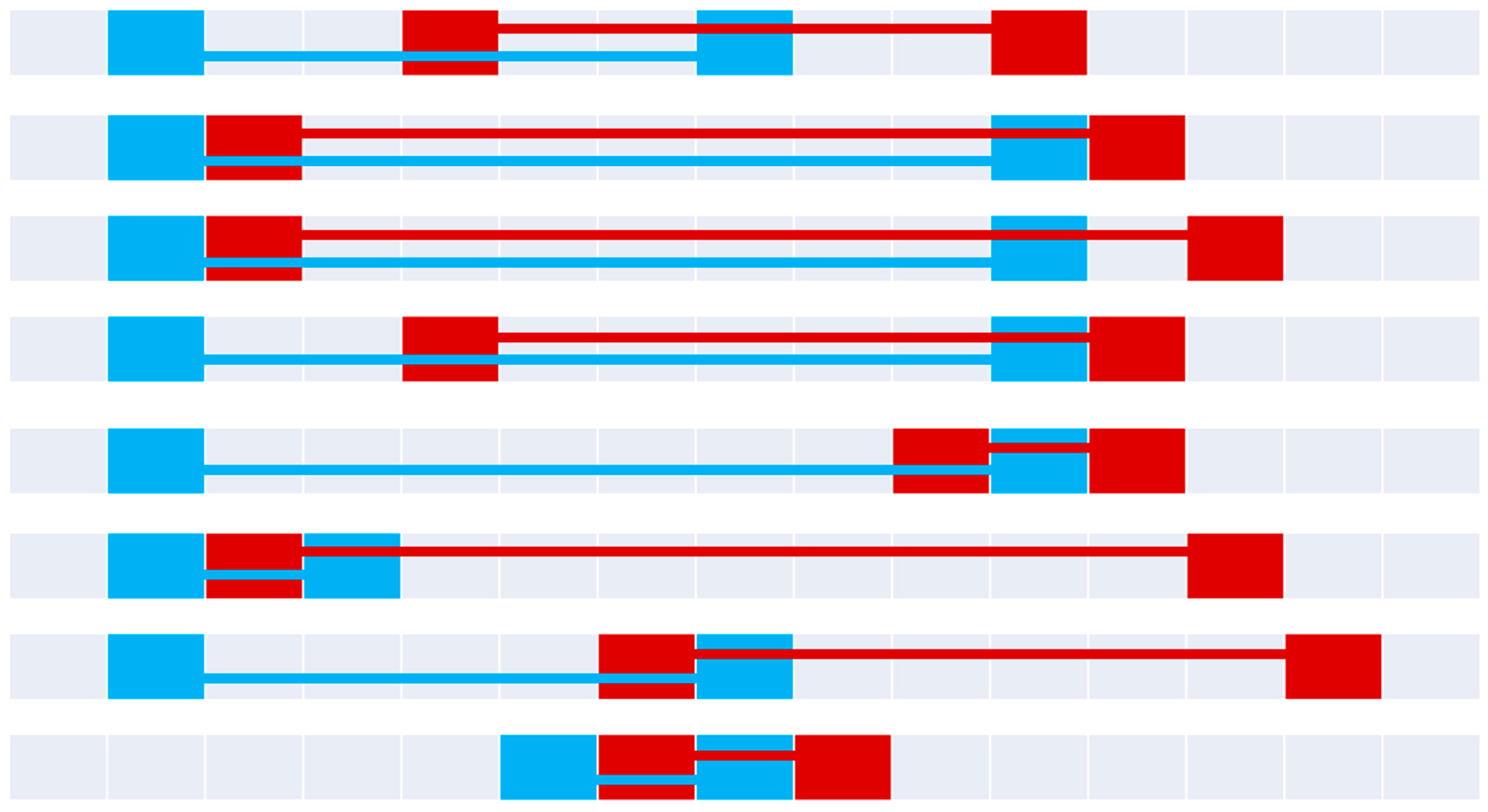
Figure 17.
Touch relations in (top to bottom): disjointTouch, disjointTouchNoAInterior, disjointTouchNoBInterior, disjointTouchNoInterior, containsTouch, containsTouchNoInterior, insideTouch, and insideTouchNoInterior. Each of these relations is anti-symmetric, resulting in a bifurcated temporal relation.
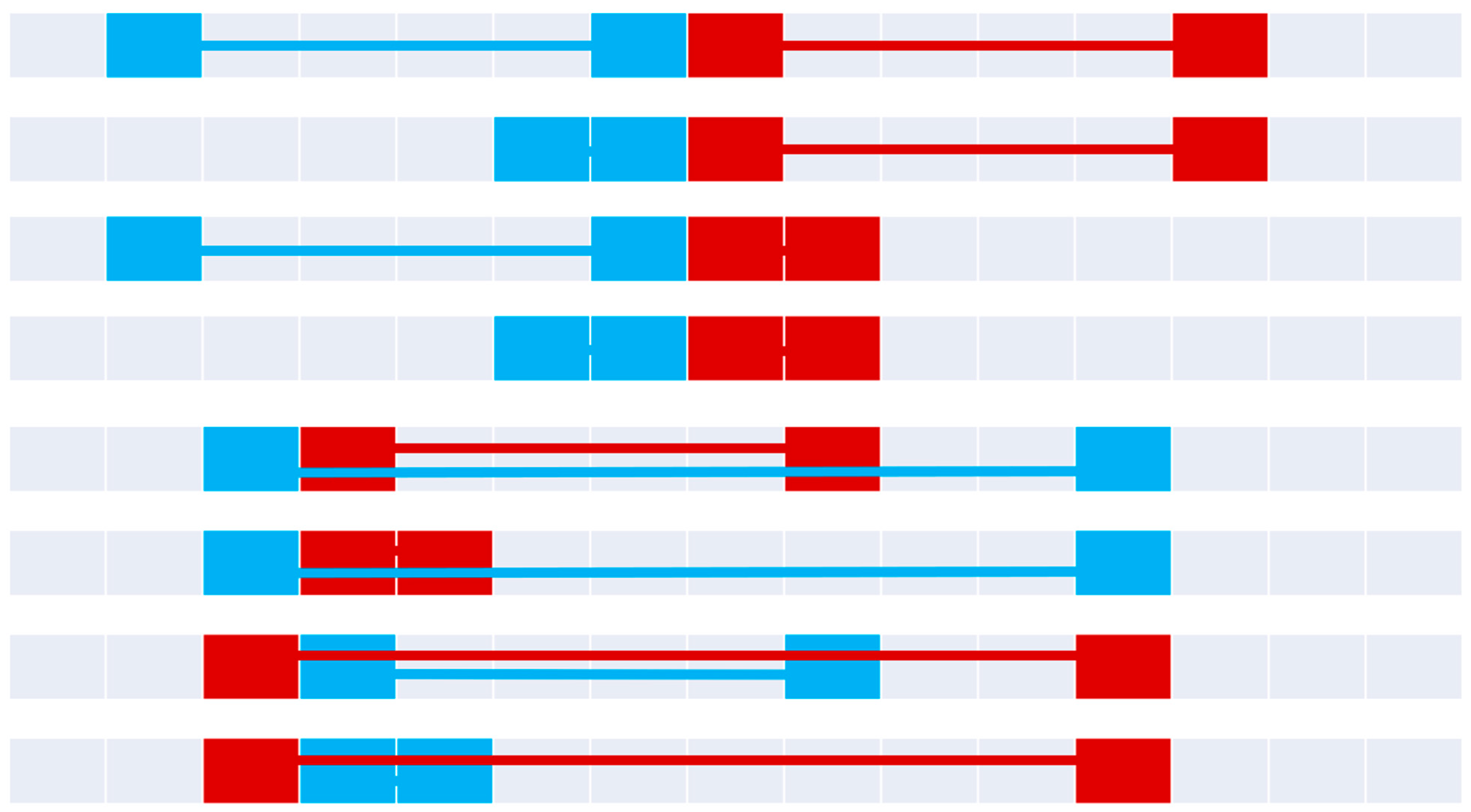
Figure 20.
Touch relations.
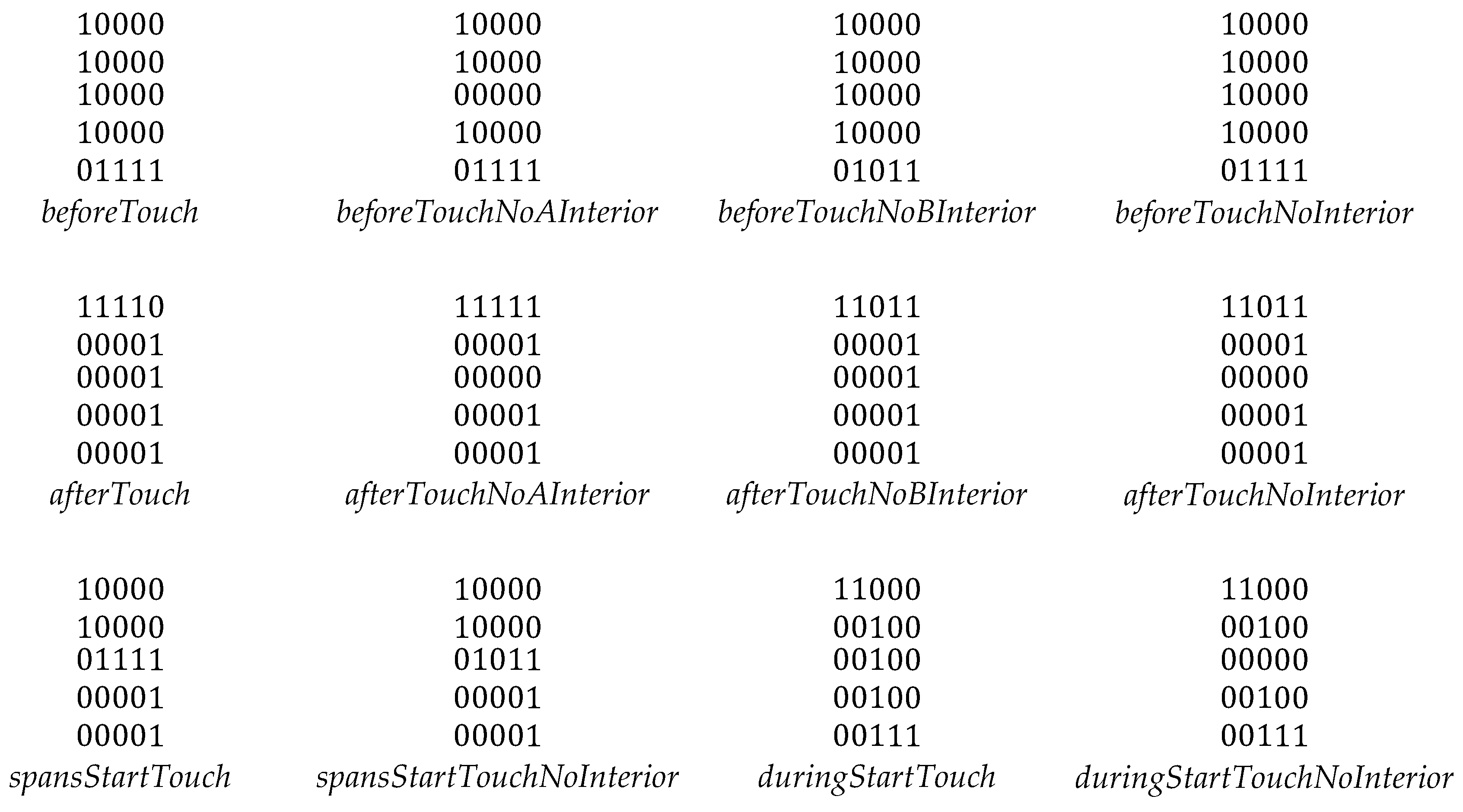
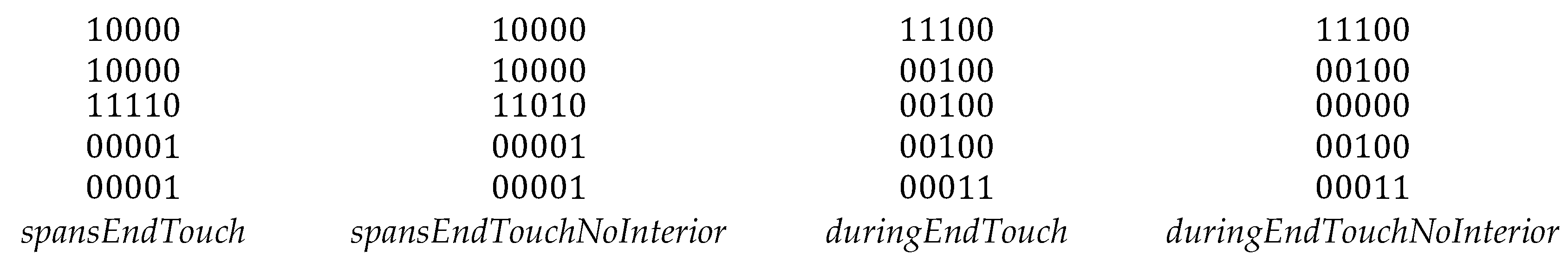

Table 1.
Existing topological relation sets for simple polygons and lines in various spaces.
| Space | Lines | Polygons | Polygons/Lines |
|---|---|---|---|
|
|
[7] | - | - |
|
|
[14,15] | [8,9,11] | [16] |
|
|
[17] | - | - |
|
|
[14,15]* | [18,19] | [16]* |
|
|
not identified | - | - |
|
|
not identified | [20,21,22,23] | not identified |
|
|
not identified | - | - |
|
|
not identified | [24] | not identified |
Disclaimer/Publisher’s Note: The statements, opinions and data contained in all publications are solely those of the individual author(s) and contributor(s) and not of MDPI and/or the editor(s). MDPI and/or the editor(s) disclaim responsibility for any injury to people or property resulting from any ideas, methods, instructions or products referred to in the content. |
© 2025 by the authors. Licensee MDPI, Basel, Switzerland. This article is an open access article distributed under the terms and conditions of the Creative Commons Attribution (CC BY) license (http://creativecommons.org/licenses/by/4.0/).
Copyright: This open access article is published under a Creative Commons CC BY 4.0 license, which permit the free download, distribution, and reuse, provided that the author and preprint are cited in any reuse.


