
Submitted:
04 July 2025
Posted:
07 July 2025
You are already at the latest version
Abstract
The necessity of modeling the dynamics of infectious disease spread is predicated on the imperative to accurately predict epidemics and assess the efficacy of control measures, such as isolation and quarantine. Conventional compartmental models have been widely used for predicting the course of epidemics, but they have limitations due to their inability to account for dynamic isolation. In this paper, we propose a novel approach based on the concept of a Working Set, which we utilize as a subset of agents actively involved in social contact and potential transmission. Our adapted Working Set model incorporates isolation states for susceptible and infected agents, enabling dynamic adjustment of the transmission rate according to the current size of the working set. The incorporation of a time window parameter enables the identification of current contacts and the identification of super-spreaders, a important component for the optimization of epidemiological measures. Experimental results show that compared to the compartmental models, our model provides a more detailed and realistic tool for analyzing the spread of infection under dynamic control measures. The presented approach integrates resource management principles from computer systems with epidemiological models, providing a flexible and realistic tool for evaluating and optimizing infectious disease control measures.
Keywords:
working set
; compartmental models
; complex systems
; epidemic spreading
; computer simulations.
1. Introduction
Compartmental models, such as SIR, SEIR, and SEIR-V have been widely used to study infectious disease outbreaks [1,2,3,4]. These models are successive mathematical extensions, each adding new aspects to more accurately model and analyze the spread of infectious diseases. They divide populations into groups (compartments) based on disease status and use differential equations to describe the transitions between them. The SIR model proposed in Kermack et al. [5] is a seminal work in the field of infectious disease modeling. In their article, Kermack and McKendrick introduced a foundational epidemiological model that segments the population into three compartments: Susceptible (S), Infected (I), and Recovered (R). This model is widely known as the Susceptible-Infected-Recovered (SIR) model. Notably, as a special case of their general framework, the authors proposed a simple system of Ordinary Differential Equations (ODEs) to describe the time evolution of population proportions in each compartment of the SIR model [6,7]. However, the classical SIR model is not entirely realistic because it assumes that individuals immediately become infectious upon exposure, while most infectious or transmittable diseases have an incubation period. The incubation period can be incorporated into the SIR framework by adding an additional compartment, resulting in the Susceptible-Exposed-Infected-Recovered (SEIR) system, which accounts for exposed or incubating individuals [8,9]. Although the SIR model is mathematically simpler and sometimes more convenient to analyze, it lacks epidemiological and biological realism [10]. Conversely, realistic data from infectious disease studies often derive from SEIR-like models, which present more modeling challenges [11,12,13]. An extended version of SEIR is the SEIR-V model, which adds the Vaccinated category V to account for the effect of vaccination on the spread of infection [14,15]. For greater accuracy, SEIR-V is often combined with agent-based models to account for individual differences in behavior and social networks [16,17]. However, the SIR, SEIR, and SEIR-V models have limitations especially in the context of dynamic control measures such as isolation or quarantine, because they assume that all susceptible and infected agents interact [18,19,20,21]. These models do not take into account how isolation can reduce contacts and thus the rate of spread. To model isolation and quarantine, the SIR and SEIR models need to be extended by adding additional states, as shown in [22].
We propose an adapted Working Set model originally developed in computer science, namely in memory management systems. The Working Set (WS) model, proposed by P. Denning [23,24], describes the set of memory pages that are actively used by a process at a given time, and the unloading of infrequently used pages. It is used to minimize page faults and improve system performance. The WS of a process is defined as the set of memory pages used during a given time interval. It is formally written as , where - is the current time and is the length of the time window. If a page is used frequently during , it is not excluded from the working set. Our primary objective is to demonstrate the application of a Working Set model to an epidemiological context. We define a "Working Set" as a subset of agents in contact with each other, among which there may be agents actively involved in contact transmission. We use this model to analyze epidemic dynamics and to evaluate the effectiveness of control measures such as isolation. In our adapted WS model, agents actively involved in transmission are excluded from the WS, i.e., isolated from the group. Thus, the algorithm of the WS model is used as a way to identify super-spreaders [25], that transmit infection to a large number of susceptible agents through frequent contact, communication, or inter-agent contact. Unlike classical models such as SIR or SEIR, our adaptive WS model accounts for dynamic isolation and varying transmission rates depending on the size of the working set. The adaptive WS model includes isolation as a central element, where agents can be removed from the working set, thereby reducing the transmission potential. Several studies show [26,27,28,29] that isolation and quarantine are important in preventing the spread of infection during epidemics. They are important tools during epidemics because they prevent the spread of disease, protect vulnerable groups, allow time for monitoring and treatment, reduce the burden on health systems, facilitate contact tracing, and have proven historical effectiveness. Despite the potential social and economic costs, their benefits in controlling epidemics are significant, making them an integral part of public health strategies. Therefore, this paper proposes an adaptation of the WS model to an epidemiological context in order to model the dynamics of infectious disease spread under various control measures.
2. Methods
We first review the basic SIR model of Kermack and McKendrick, where the proportions of agents in susceptible, infected, and removed compartments satisfy the following system of ODEs:
where: - disease transmission rate, representing the average number of contacts per agent per unit time multiplied by the probability of transmission; - is the recovery rate, representing the average rate at which infected individuals recover; - the total population size held constant in the base model.
The key parameter is the base reproductive rate , calculated as . Here is the average number of secondary infections caused by an infected individual in a fully susceptible population. If the disease spreads, if it dies out.
SEIR (with incubation period):
where: - is the to transition coefficient, i.e. the rate at which exposed individuals become infectious (1/ is the average duration of the latency period); and - are similar to the SIR model. The base reproductive rate for SEIR is calculated as:
where - is the natural mortality rate, which may be zero in simplified models.
2.1. Details of the Model
We now examine some key assumptions of adapted WS model to epidemiology. Key elements of the original WS model are redefined as follows: Population: The complete set of agents in a system, analogous to the set of all memory pages in a computer model. Working set: A subset of the population that includes agents that are not currently isolated and may be involved in transmission. Isolation: The process of excluding agents from the working set, equivalent to unloading pages from RAM. Isolated agents are temporarily not involved in the spread of infection. Super-spreader: An infected agent (in state ) that transmits infection to an unusually large number of susceptible agents (state ). Unlike the average infected agent, a super-spreader causes significantly more infections due to high contact frequency or other factors.
2.2. Definition of States in the Model
The adapted model introduces the following states that reflect the epidemiologic status of the agents: Susceptible (): Agents that can become infected through contact with infected agents. Infected (): Agents capable of transmitting infection to others. Recovered (): Agents who have developed immunity and are no longer involved in transmission. Isolated (): These are infected agents or, in rare cases, susceptible agents that are physically separated from the rest to prevent further spread of the disease. The adaptive WS model is described by a system of ordinary differential equations (ODEs):
where, - isolated susceptible; - isolated infected; - isolated recovered (transferred from after recovery); - dynamic infection rate; - current working set size (sum of agents in states and ) at time t; - isolation rate for ; - isolation rate for ; - isolation escape velocity for ; - isolation escape velocity for ; - rate of recovery. This system accounts for all key processes: infection, recovery, isolation and release. The total population in the model is defined as follows: The size of the working set is determined by the formula:
2.3. Dynamics of Transitions Between States
The dynamics of infection spread in the model is determined by the following processes:
- Infection: Transition of agents from state to by contact with infected agents. The speed of this process depends on the frequency of contact and the probability of transmission:
- Recovery: Transition from to as infected agents recover. Rate of transition from to will be:
- Isolation: The transfer of agents from or to as a result of control measures such as contact tracing or isolation. Then the coefficient from to will be: . And from to will be: .
- Release from isolation: Return of agents from to (if they remain susceptible) or to (if recovered) after completion of the isolation period or confirmation of status by calculating: . From to (recovery in isolation): . From to will be: .
2.4. Impact on the Rate of Transmission of Infection
In contrast to traditional models such as SIR, where the infection rate is assumed to be constant and the population is assumed to be homogeneously mixed, in the adapted WS model the value of becomes a dynamic variable depending on the size of the working set:
where: - is basic transmission rate under full population conditions.
As the number of isolated agents increases, the size of the WS decreases, which reduces and slows the spread of infection. This approach allows us to model the effect of isolation and other control measures on epidemic dynamics. Human populations are heterogeneous in many aspects: social connections among agents display clustered community patterns [30,31,32], susceptibility and infectiousness potential vary widely due to age, health, or behavioral differences, and geographic regions often implement distinct epidemic containment strategies. The long-standing assumption of uniform, well-mixed populations has been rigorously tested through heterogeneous modeling frameworks [33,34,35,36,37]. To summarize the effects of uneven transmission likelihoods, vulnerability distributions, and interaction patterns, we use a simple class of models in which the population is partitioned into multiple groups of agents [38,39,40]. These adaptations aim to demonstrate that population diversity can significantly alter both the progression and total reach of an epidemic, and, critically, broaden the range of viable intervention strategies.
Let consider a multi-agent system (MAS) with n agents distributed over p groups and exposed to the risk of infection through contact with each other. In our understanding, MAS consists of a finite number of agents and an environment that hosts agents in which agents act and react to other agents. Let specify that the agents' distribution into groups, and each agent group number can be easily determined by the Boolean matrix , where the element is , if the agent with the number is located in the group with the number r and , otherwise. The matrix must satisfy constraints (a), (b), and (c). Whatever the distribution of agents over groups, we assume that each agent of the system belongs to only one of the groups (condition, (a)):
Each agent of the system is assigned a weight, the linear size of its living space, within which the agent can perform its set of operations assigned to it. In this case, the agents interacting with each other are exposed to infection risk through contact. Each group is also assigned a weight - living space within which the group's agents are located. The total weight of agents in any group should not exceed the weight of the group (condition (b)):
Here is the weight of the agent , and is the weight of the group with number r, r=1, 2, ... , p. Let determine the number of a group that contains an agent, for example , with a given matrix , denoting this number by and taking into account the constraints , we write:
3. Modeling and Results
A WS in an epidemiological context is a dynamic group of agents that participate in social interactions and are not subject to isolation. Its size and composition depend on the following factors: Isolation policy: When an infected agent from is identified, its contacts from in the last days are relegated to the state . This shortens the WS and reduces the likelihood of new infections. At the end of the isolation period, agents from are tested: susceptible agents return to , recovered agents to . An alternative scenario is high-coverage isolation, in which a large fraction of the population is isolated. Time window (): Similar to the original WS model, a parameter is introduced to define the period of "relevance" of contacts. Agents who have been in contact with infected agents in the last time units are considered candidates for isolation. There may also be superspreaders among these agents. Their identification is important for epidemic control because isolation of such agents can significantly slow the spread of the disease. In the WS model, the parameter specifies the time window during which contacts are considered relevant.
3.1. Numerical Simulations
To assess the dynamics of infection spread and evaluate the impact of isolation measures. To focus on the isolation period and the effectiveness of the various scenarios, we started creating three different scenarios. For this purpose, we introduce experimental scenarios of isolation rate: 1. Basic scenario: No isolation (, ); 2. Moderate isolation: Low isolation parameters (, ); 3. High-coverage isolation: High isolation parameters (, ). The SIR and SEIR models do not take insulation into account, so only the basic scenario is considered. Table 1 shows the values of parameters and descriptions used for numerical simulations.
We used an agent-based model that allows us to model different strategies in a virtual population and compare these strategies to get an idea of their optimal parameters. Multi-agent modeling is a method of simulating the behavior of multiple agents interacting in with each other in environment [41,42]. By modeling spread of an infection, we are able to trace a typical epidemiological dynamic that progresses through several key stages. Figure 1 illustrates the dynamics of the epidemic spread process considering five types of agents: Blue - susceptible agents; Orange - infected agents; Red - super-spreaders; Black - isolated agents; Gray - recovered agents.
As illustrated in Figure 1(a), the initial stage of the epidemic is characterized by a population consisting predominantly of susceptible agents, with an infection rate that is just beginning to manifest due to a limited number (0.3%) of infected agents. As shown in Figure 1(b), as the epidemic progresses, the proportion of infected agents increases to 2.4%, the first isolated agents appear, amount of which is 0.08% and super-spreaders emerge at 0.18% in 10 days. These superspreaders play a critical role by rapidly infecting the surrounding community and forming the first foci of infection, in this case, clusters of agents. In the early stages of an outbreak, local foci of infection emerge around each superspreader, as illustrated by the red circles. As illustrated in Figure 1(c), the proportion of infected agents increases to 18%, the number of isolated agents rises to 11%, and the proportion of superspreaders increases to 13%. As the epidemic progresses, small foci coalesce into a "cluster network," and transmission "bridges" between groups of agents emerge, thereby accelerating the spread of the infection. As illustrated in Figure 1(d), the initial recovered agents that were released following the isolation period are represented by the gray squares. The number of susceptible agents experiences a substantial decrease. At the peak of the epidemic, as shown in Figure 1(e), the proportion of susceptible agents constitutes - 0.2% of the total population. The proportion of infected agents reaches - 12%, the super-spreaders - 51%, isolated agents – 26%, recovered agents - 10.8% on day 59. The implementation of more stringent isolation protocols at this juncture emerges as a pivotal factor in the mitigation of the propagation of infection. The proportion of isolated agents stands at 38%, thereby impeding the further dissemination of the infection. In Figure 1(g), the proportion of infected agents is approximately 5%, super-spreaders account for 41%, and isolated comprise about 21%. The proportion of recovered agents is 32%. As illustrated in Figure 1(h), the final stage of the infection virtually disappears, and all agents are recovered within 100 days. The simulations underscore the pivotal function of super-spreaders in expediting the propagation of the epidemic and the paramount importance of prompt isolation measures in its control, a phenomenon that is vividly illustrated by the dynamics depicted in the figures.
Figure 2 (a) shows a comparison of the dynamics of infected agents in the basic scenario for SIR, SEIR, and Working Set (without isolation). The SIR model shows a rapid increase in infections with a peak of 3049 on day 26, followed by a sharp decline. SIR shows the fastest and most intense epidemic due to the lack of delay in infection. In the SEIR model, the peak is lower, around 20,000 and later, around day 51, due to the incubation period. SEIR slows the spread by exposing, lowering, and delaying the peak. The WS model results are consistent with SIR because there is no isolation. This confirms the correctness of the WS implementation in the absence of isolation, on par with SIR. Figure 2 (b) shows the dynamics of infected agents in the WS model for the three isolation scenarios. Without isolation, the peak of infected agents is 3050 on day 26. With moderate isolation, the peak drops to 755 and shifts to day 59. With high-coverage isolation, the peak shows 100 at the beginning, and then gradually decreases. The results show that isolation effectively "flattens the curve", reducing the peak of infection and slowing the epidemic. The high-coverage isolation with parameters , is most effective, reducing the peak by a factor of three and allowing more time for preparation. Figure 2 (c) shows the evolution of all states of the WS model with moderate isolation. The value of S decreases more slowly than in SIR due to the isolation. The number of recoveries increases to 7800 in the end. The peak of infected agents is about 2400 on day 20 and then declines steadily. This means that detection and isolation of super-spreaders plays a key role in controlling peak infections. As shown in Figure 2 (d), the number of recovered (R) for the WS is much lower than SIR and SEIR. This is because the number of infected was lower due to isolation, and consequently the number of cured is also lower. Isolation in the WS reduces the final size of the epidemic by preventing part of the population from being infected, while the SIR and SEIR models show larger epidemics due to the lack of isolation.
In Figure 3 shown epidemic sensitivity heatmaps of the Working Set model. Figure 3 (a) shows the final recovery rate as a function of the infection rate and recovery rate parameters. Figure 3 (b) the analysis of the parameters of isolation of infected people, which is more effective in reducing the peak. But at the same time, strong isolation can significantly reduce the burden on the health system [43,44,45,46] or economy [47]. Figure 3 (c) shows the rate of isolation release for the WS. A fast release from isolation increases the size of the epidemic as people return to the active population. A slow release keeps the epidemic under control, but requires more resources.
Thus, comparing the SIR, SEIR, and WS models, we can say that WS is flexible due to isolation, which makes it more realistic for modeling control measures. To evaluate the efficiency of the adapted WS model, we compare it with the classical SIR and SEIR models.

Table 2.
Comparison results of models.
| Aspect | SIR/SEIR | WS |
| Isolation | Not directly accounted, expansion required |
Included as centerpiece, dynamic adjustment |
| Transmission speed | Fixed or dependent on S and I | Dynamically adjusted based on active set |
| Contact heterogeneity | Requires extensions (e.g. network) | Accounting through groups and subsets |
| Behavioral solutions | Not modeled | May be enabled via agent rules |
| Applicability for interventions |
Limited without modifications | Easy to model isolation |
Theorem-type environments (including propositions, lemmas, corollaries, etc.) can be formatted as follows Сomparing the SIR, SEIR, and WS models, we can say that WS is flexible due to isolation, which makes it more realistic for modeling control measures. The proposed WS model has several advantages like accounting for contact heterogeneity and ability to quantify the impact of isolation, contact tracing, and other strategies. Also, similar to memory management in computer science, the model allows us to explore the effectiveness of epidemic control. These analyses demonstrate how an adapted WS model can be useful in investigating epidemic dynamics, providing valuable insights for infectious disease management. Further investigation of the model might be useful for health planning and evaluating measures such as isolation and social distancing.
4. Conclusions
Epidemic modeling is a useful tool for understanding and controlling the spread of infectious diseases. The proposed Working Set model adapted to the epidemiological context offers a new approach to modeling the spread of infectious diseases and shows the potential to improve the realism and responsiveness of epidemiological modeling, especially in the context of dynamic control measures such as isolation and quarantine. Unlike classical SIR and SEIR models, our model allows us to identify an active subset of agents as a "Working Set" that are directly involved in the transmission of infection. This approach allows us to account for heterogeneity in social contacts and to identify super-spreaders, which is important for slowing epidemic growth. The introduction of dynamic isolation mechanisms allows more accurate modeling of the impact of control measures on the rate of disease spread. Despite some advantages, the WS model has certain limitations, including the complexity of the mathematical apparatus, the need for accurate empirical data, and detailed parameter calibration. Nevertheless, this approach, which combines resource management principles from computer science with epidemiological problems, offers prospects for the development of optimal epidemic control strategies.
Thus, the adapted Working Set model is a promising tool for analyzing and managing the spread of infectious diseases. Its use can facilitate more accurate assessment of the impact of control measures, development of optimal isolation strategies, and timely response to epidemic threats. This study could help in the modeling of other similar diseases. Further research in this area will improve the model and integrate it with other approaches to improve public health planning in a rapidly changing epidemiological environment.
Author Contributions
The authors confirm contribution to the paper as follows: Conceptualization, A.M. and G.B.; methodology, A.M. and A.T; software, A.M; validation, Z.T., A.M. and G.B.; formal analysis, S.D.; investigation, Z.T.; resources, N.Z.; data curation, A.M.; writing—original draft preparation, A.M. and G.B; writing—review and editing, A.M. and A.T; visualization, Z.T.; supervision, A.M.; project administration, G.B.; funding acquisition, A.M. and G.B. All authors have read and agreed to the published version of the manuscript.
Funding
This research was funded by a grant from the Science Committee of the Ministry of Science and Higher Education of the Republic of Kazakhstan, grant number “AP19174930”.
Institutional Review Board Statement
Not applicable.
Informed Consent Statement
Not applicable.
Data Availability Statement
Data can certainly be provided upon request.
Conflicts of Interest
The authors declare no conflicts of interest.
References
- Billah, M.A.; Miah, M.M.; Khan, M.N. Reproductive Number of Coronavirus: A Systematic Review and Meta-Analysis Based on Global Level Evidence. PLOS ONE 2020, 15, e0242128. [Google Scholar] [CrossRef] [PubMed]
- Pastor-Satorras, R.; Castellano, C.; Van Mieghem, P.; Vespignani, A. Epidemic Processes in Complex Networks. Rev. Mod. Phys. 2015, 87, 925–979. [Google Scholar] [CrossRef]
- Hethcote, H.W. The Mathematics of Infectious Diseases. SIAM Rev. 2000, 42, 599–653. [Google Scholar] [CrossRef]
- Siegenfeld, A.F.; Kollepara, P.K.; Bar-Yam, Y. Modeling Complex Systems: A Case Study of Compartmental Models in Epidemiology. Complexity 2022, 2022, 3007864. [Google Scholar] [CrossRef]
- Kermak, W.O; McKendrick, A.G. A Contribution to the Mathematical Theory of Epidemics. Proc. R. Soc. Lond. A 1927, 115, 700–721. [Google Scholar] [CrossRef]
- Sun, R. Global Stability of the Endemic Equilibrium of Multigroup SIR Models with Nonlinear Incidence. Computers & Mathematics with Applications 2010, 60, 2286–2291. [Google Scholar] [CrossRef]
- Turkyilmazoglu, M. A Highly Accurate Peak Time Formula of Epidemic Outbreak from the SIR Model. Chinese Journal of Physics 2023, 84, 39–50. [Google Scholar] [CrossRef]
- KhudaBukhsh, W.R.; Rempała, G.A. How to Correctly Fit an SIR Model to Data from an SEIR Model? Mathematical Biosciences 2024, 375, 109265. [Google Scholar] [CrossRef]
- Korobeinikov, A. Global Properties of SIR and SEIR Epidemic Models with Multiple Parallel Infectious Stages. Bull. Math. Biol. 2009, 71, 75–83. [Google Scholar] [CrossRef]
- Lara-Tuprio, E.P.D.; Estadilla, C.D.S.; Teng, T.R.Y.; Uyheng, J.; Estuar, M.R.J.E.; Espina, K.E.; Macalalag, J.M.R.; Sarmiento, R.F.R. Mathematical Analysis of a COVID-19 Compartmental Model with Interventions.; Penang, Malaysia, 2021; p. 020025.
- Gumel, A.B.; Iboi, E.A.; Ngonghala, C.N.; Elbasha, E.H. A Primer on Using Mathematics to Understand COVID-19 Dynamics: Modeling, Analysis and Simulations. Infectious Disease Modelling 2021, 6, 148–168. [Google Scholar] [CrossRef]
- Yan, P.; Chowell, G. Beyond the Initial Phase: Compartment Models for Disease Transmission. In Quantitative Methods for Investigating Infectious Disease Outbreaks; Springer International Publishing: Cham, 2019; Volume 70, pp. 135–182. ISBN 9783030219222 9783030219239. [Google Scholar]
- Marques, J.A.L.; Gois, F.N.B.; Xavier-Neto, J.; Fong, S.J. Epidemiology Compartmental Models—SIR, SEIR, and SEIR with Intervention. In Predictive Models for Decision Support in the COVID-19 Crisis; Springer International Publishing: Cham, 2021; pp. 15–39. ISBN 9783030619121. [Google Scholar]
- Meng, X.; Cai, Z.; Si, S.; Duan, D. Analysis of Epidemic Vaccination Strategies on Heterogeneous Networks: Based on SEIRV Model and Evolutionary Game. Applied Mathematics and Computation 2021, 403, 126172. [Google Scholar] [CrossRef] [PubMed]
- Safarishahrbijari, A.; Lawrence, T.; Lomotey, R.; Liu, J.; Waldner, C.; Osgood, N. Particle Filtering in a SEIRV Simulation Model of H1N1 Influenza. In Proceedings of the 2015 Winter Simulation Conference (WSC); December 2015; pp. 1240–1251. [Google Scholar]
- Bissett, K.R.; Cadena, J.; Khan, M.; Kuhlman, C.J. Agent-Based Computational Epidemiological Modeling. J Indian Inst Sci 2021, 101, 303–327. [Google Scholar] [CrossRef] [PubMed]
- Salem, F.A.; Moreno, U.F. A Multi-Agent-Based Simulation Model for the Spreading of Diseases Through Social Interactions During Pandemics. J Control Autom Electr Syst 2022, 33, 1161–1176. [Google Scholar] [CrossRef]
- Tolles, J.; Luong, T. Modeling Epidemics With Compartmental Models. JAMA 2020, 323, 2515. [Google Scholar] [CrossRef]
- Roberts, M.; Andreasen, V.; Lloyd, A.; Pellis, L. Nine Challenges for Deterministic Epidemic Models. Epidemics 2015, 10, 49–53. [Google Scholar] [CrossRef]
- Givan, O.; Schwartz, N.; Cygelberg, A.; Stone, L. Predicting Epidemic Thresholds on Complex Networks: Limitations of Mean-Field Approaches. Journal of Theoretical Biology 2011, 288, 21–28. [Google Scholar] [CrossRef]
- Dhar, A. What One Can Learn from the SIR Model. iascs 2020, 3. [Google Scholar] [CrossRef]
- Džiugys, A.; Bieliūnas, M.; Skarbalius, G.; Misiulis, E.; Navakas, R. Simplified Model of Covid-19 Epidemic Prognosis under Quarantine and Estimation of Quarantine Effectiveness. Chaos Solitons Fractals 2020, 140, 110162. [Google Scholar] [CrossRef]
- Denning, P. J. The working set model for program behavior, in Proceedings of the ACM symposium on Operating System Principles - SOSP ’67, Not Known: ACM Press, 1967, p. 15.1-15.12. [Google Scholar] [CrossRef]
- Denning, P.J. Working Set Analytics. ACM Comput. Surv. 2021, 53, 1–36. [Google Scholar] [CrossRef]
- Lloyd-Smith, J.O.; Schreiber, S.J.; Kopp, P.E.; Getz, W.M. Superspreading and the Effect of Individual Variation on Disease Emergence. Nature 2005, 438, 355–359. [Google Scholar] [CrossRef]
- Dénes, A.; Gumel, A.B. Modeling the Impact of Quarantine during an Outbreak of Ebola Virus Disease. Infect Dis Model 2019, 4, 12–27. [Google Scholar] [CrossRef] [PubMed]
- Poonia, R.C.; Saudagar, A.K.J.; Altameem, A.; Alkhathami, M.; Khan, M.B.; Hasanat, M.H.A. An Enhanced SEIR Model for Prediction of COVID-19 with Vaccination Effect. Life (Basel) 2022, 12, 647. [Google Scholar] [CrossRef] [PubMed]
- Ramalingam, R.; Gnanaprakasam, A.J.; Boulaaras, S. Stability and Control Analysis of COVID-19 Spread in India Using SEIR Model. Sci Rep 2025, 15, 9095. [Google Scholar] [CrossRef] [PubMed]
- James, A.; Plank, M.J.; Hendy, S.; Binny, R.; Lustig, A.; Steyn, N.; Nesdale, A.; Verrall, A. Successful Contact Tracing Systems for COVID-19 Rely on Effective Quarantine and Isolation. PLoS ONE 2021, 16, e0252499. [Google Scholar] [CrossRef]
- Girvan, M.; Newman, M.E.J. Community Structure in Social and Biological Networks. Proc. Natl. Acad. Sci. U.S.A. 2002, 99, 7821–7826. [Google Scholar] [CrossRef]
- Arenas, A.; Danon, L.; Diaz-Guilera, A.; Gleiser, P.M.; Guimer, R. Community Analysis in Social Networks. The European Physical Journal B - Condensed Matter 2004, 38, 373–380. [Google Scholar] [CrossRef]
- Hedayatifar, L.; Rigg, R.A.; Bar-Yam, Y.; Morales, A.J. US Social Fragmentation at Multiple Scales. J. R. Soc. Interface. 2019, 16, 20190509. [Google Scholar] [CrossRef]
- Britton, T.; Ball, F.; Trapman, P. A Mathematical Model Reveals the Influence of Population Heterogeneity on Herd Immunity to SARS-CoV-2. Science 2020, 369, 846–849. [Google Scholar] [CrossRef]
- Gou, W.; Jin, Z. How Heterogeneous Susceptibility and Recovery Rates Affect the Spread of Epidemics on Networks. Infectious Disease Modelling 2017, 2, 353–367. [Google Scholar] [CrossRef]
- Hickson, R.I.; Roberts, M.G. How Population Heterogeneity in Susceptibility and Infectivity Influences Epidemic Dynamics. Journal of Theoretical Biology 2014, 350, 70–80. [Google Scholar] [CrossRef]
- Gerasimov, A.; Lebedev, G.; Lebedev, M.; Semenycheva, I. COVID-19 Dynamics: A Heterogeneous Model. Front. Public Health 2021, 8, 558368. [Google Scholar] [CrossRef] [PubMed]
- Dolbeault, J.; Turinici, G. Social Heterogeneity and the COVID-19 Lockdown in a Multi-Group SEIR Model. Computational and Mathematical Biophysics 2021, 9, 14–21. [Google Scholar] [CrossRef]
- Van Den Driessche, P.; Watmough, J. Reproduction Numbers and Sub-Threshold Endemic Equilibria for Compartmental Models of Disease Transmission. Mathematical Biosciences 2002, 180, 29–48. [Google Scholar] [CrossRef]
- Hébert-Dufresne, L.; Althouse, B.M.; Scarpino, S.V.; Allard, A. Beyond R0 : Heterogeneity in Secondary Infections and Probabilistic Epidemic Forecasting. J. R. Soc. Interface. 2020, 17, 20200393. [Google Scholar] [CrossRef]
- Diekmann, O.; Heesterbeek, J.A.P.; Metz, J.A.J. On the Definition and the Computation of the Basic Reproduction Ratio R 0 in Models for Infectious Diseases in Heterogeneous Populations. J. Math. Biol. 1990, 28. [Google Scholar] [CrossRef]
- Topîrceanu, A. On the Impact of Quarantine Policies and Recurrence Rate in Epidemic Spreading Using a Spatial Agent-Based Model. Mathematics 2023, 11, 1336. [Google Scholar] [CrossRef]
- Tatsukawa, Y.; Arefin, Md.R.; Kuga, K.; Tanimoto, J. An Agent-Based Nested Model Integrating within-Host and between-Host Mechanisms to Predict an Epidemic. PLoS ONE 2023, 18, e0295954. [Google Scholar] [CrossRef]
- Nitzsche, C.; Simm, S. Agent-Based Modeling to Estimate the Impact of Lockdown Scenarios and Events on a Pandemic Exemplified on SARS-CoV-2. Sci Rep 2024, 14, 13391. [Google Scholar] [CrossRef]
- Schluter, P.J.; Généreux, M.; Landaverde, E.; Chan, E.Y.Y.; Hung, K.K.C.; Law, R.; Mok, C.P.Y.; Murray, V.; O’Sullivan, T.; Qadar, Z.; et al. An Eight Country Cross-Sectional Study of the Psychosocial Effects of COVID-19 Induced Quarantine and/or Isolation during the Pandemic. Sci Rep 2022, 12, 13175. [Google Scholar] [CrossRef]
- Lin, Y.; Wu, L.; Ouyang, H.; Zhan, J.; Wang, J.; Liu, W.; Jia, Y. Behavioral Intentions and Perceived Stress under Isolated Environment. Brain and Behavior 2024, 14, e3347. [Google Scholar] [CrossRef]
- Kudriavtseva, A.S.; Arkadeva, O.G. IMPACT OF CORONAVIRUS (COVID-19) ON THE GLOBAL ECONOMY. Oecon. et jus 2022, 44–51. [Google Scholar] [CrossRef]
- Yamaka, W.; Lomwanawong, S.; Magel, D.; Maneejuk, P. Analysis of the Lockdown Effects on the Economy, Environment, and COVID-19 Spread: Lesson Learnt from a Global Pandemic in 2020. IJERPH 2022, 19, 12868. [Google Scholar] [CrossRef]
Figure 1.
The dynamics of the epidemic spread.
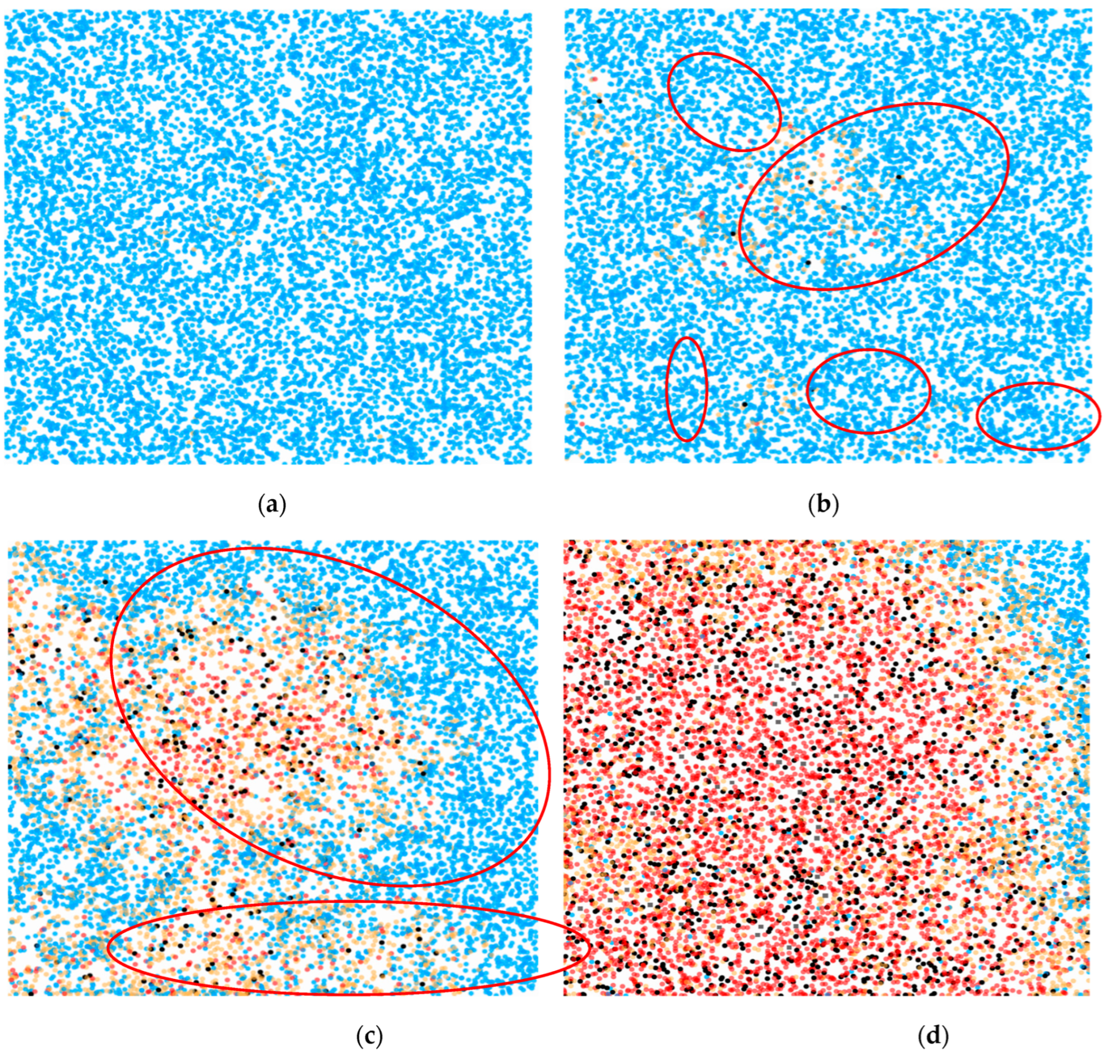
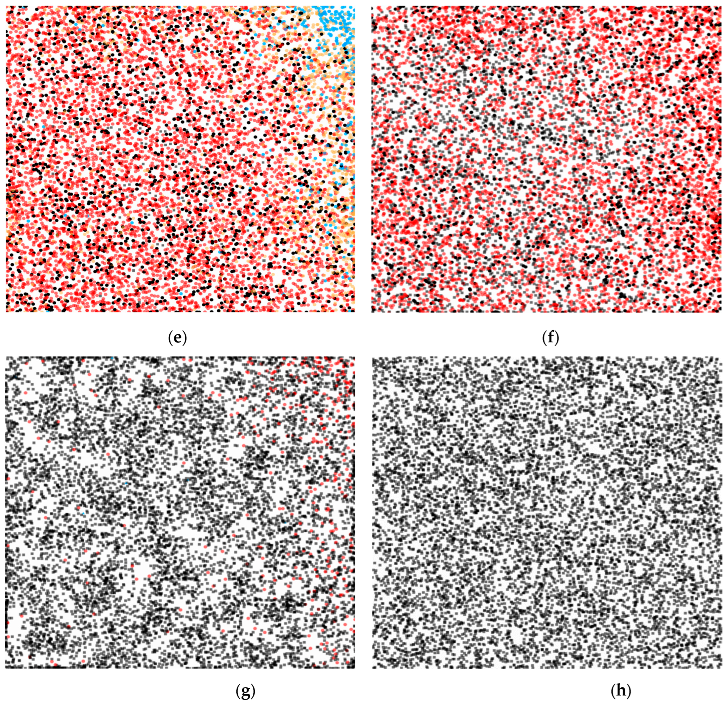
Figure 2.
Comparison of the models in different scenarios and states.
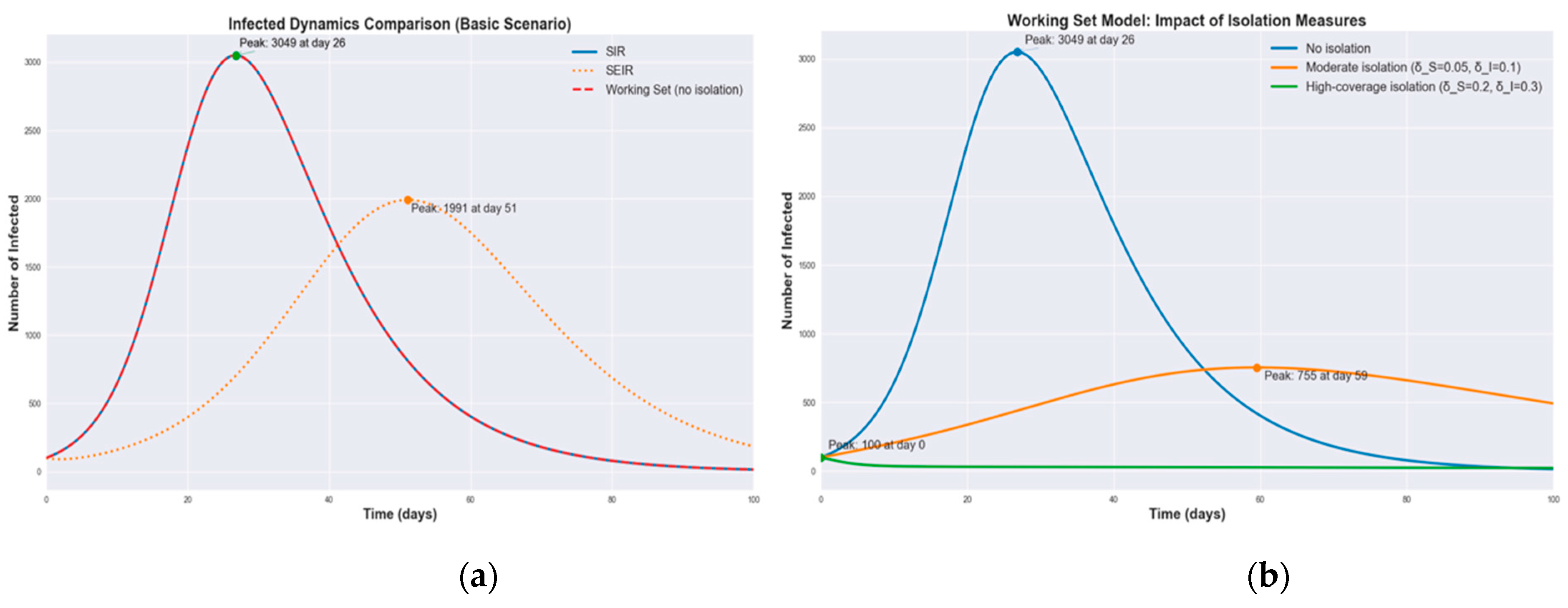
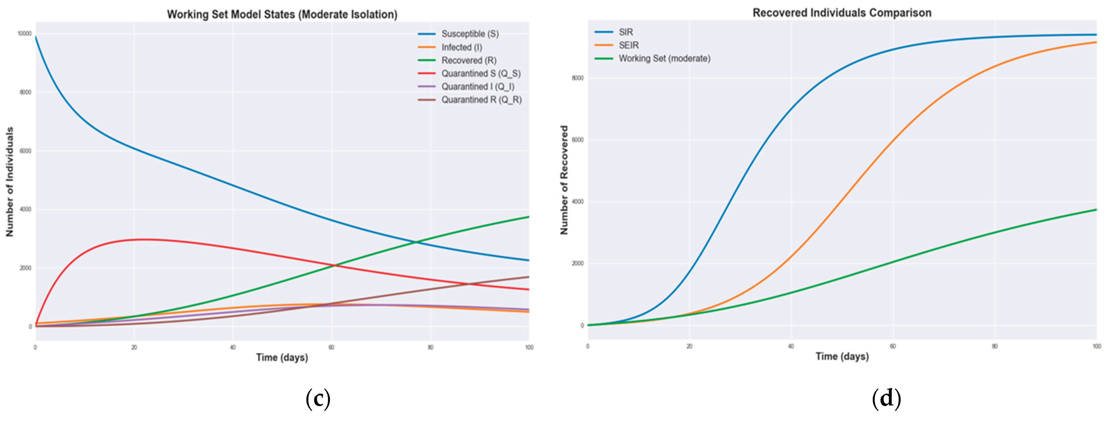
Figure 3.
Epidemic Sensitivity Heatmaps of the Working Set Model.
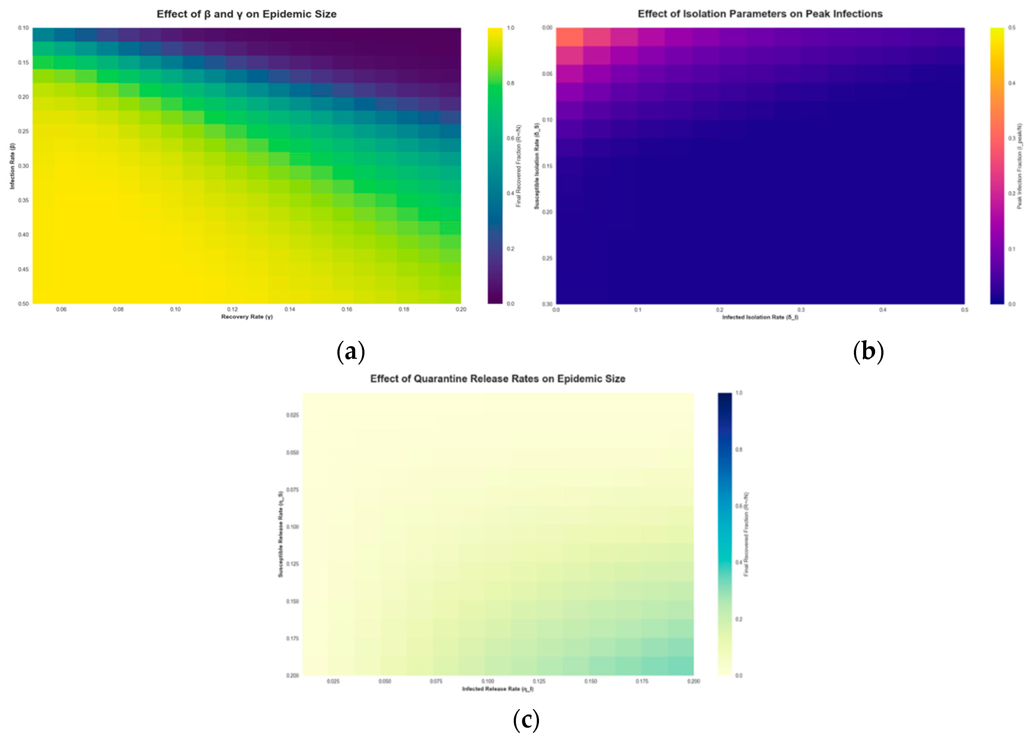
Table 1.
Model Parameters and Descriptions.
| Variable | Default value | Explanation |
|
|
10,000 | total number of agents in the population |
|
|
9970 | initial number of susceptible agents |
|
|
30 | initial number of infected agents |
|
|
0 | initial number of recovered agents |
|
|
0 | initial number of exposed agents (for SEIR model) |
|
|
0 | initial number of isolated susceptible agents |
|
|
0 | initial number of isolated infected agents |
|
|
0 | initial number of isolated recovered agents |
|
|
0.3 | infection rate; probability of disease transmission per contact between susceptible and infected agents |
|
|
0.3 | base infection rate for the working set |
|
|
0.2 | incubation rate; rate at which exposed agents become infectious (for SEIR model) |
|
|
0.1 | recovery rate; proportion of infected agents recovering per unit time |
|
|
0.1 | isolation release rate for susceptible agents; |
|
|
0.1 | isolation release rate for infected agents. |
Disclaimer/Publisher’s Note: The statements, opinions and data contained in all publications are solely those of the individual author(s) and contributor(s) and not of MDPI and/or the editor(s). MDPI and/or the editor(s) disclaim responsibility for any injury to people or property resulting from any ideas, methods, instructions or products referred to in the content. |
© 2025 by the authors. Licensee MDPI, Basel, Switzerland. This article is an open access article distributed under the terms and conditions of the Creative Commons Attribution (CC BY) license (http://creativecommons.org/licenses/by/4.0/).
Copyright: This open access article is published under a Creative Commons CC BY 4.0 license, which permit the free download, distribution, and reuse, provided that the author and preprint are cited in any reuse.


