Submitted:
08 July 2025
Posted:
08 July 2025
Read the latest preprint version here
Abstract
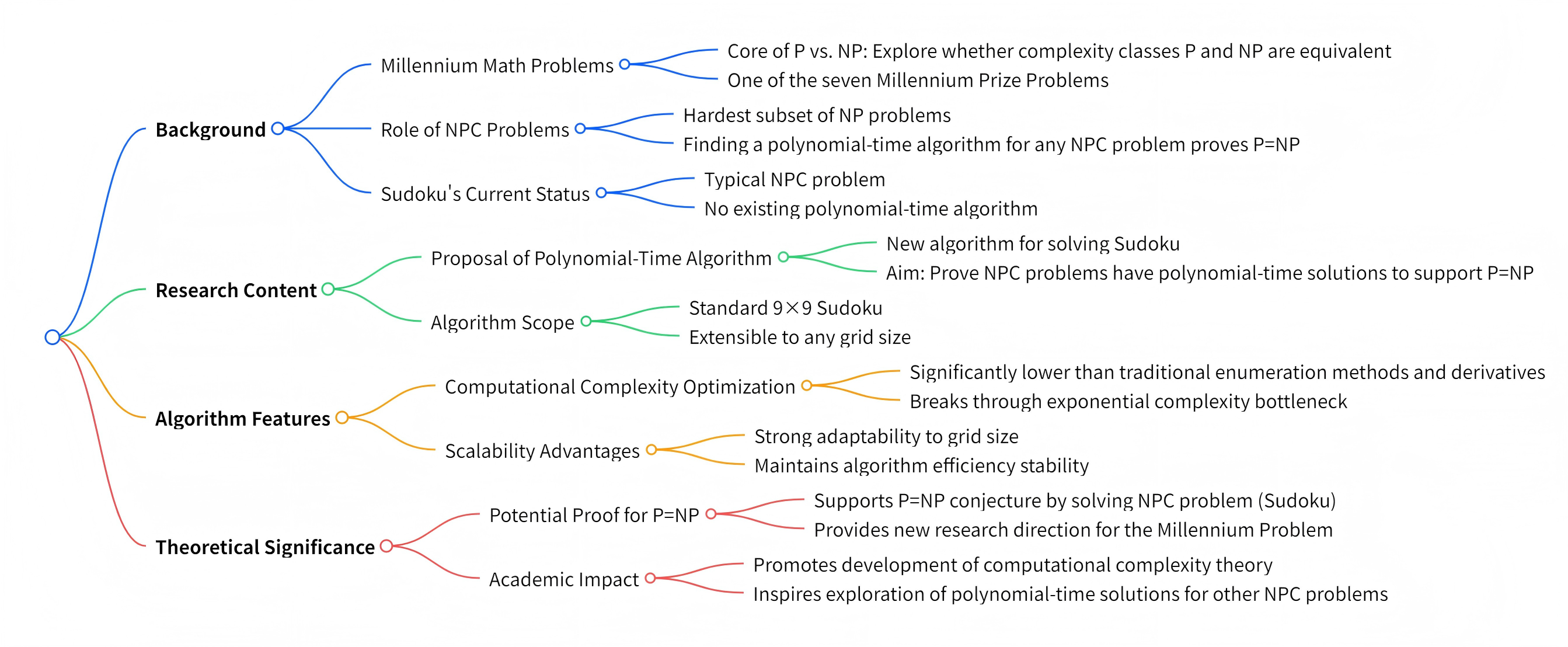
The P vs. NP equivalence problem, one of the seven major mathematical challenges of the millennium, continues to challenge researchers in mathematics and computer science. At its core, this question explores whether the complexity classes P and NP are equivalent. NPC problems, the most challenging subset of NP problems, can lead to the proof that P=NP if a polynomial-time algorithm is found for any of them. The Sudoku solving problem, a typical NPC problem, has yet to be solved using a polynomial-time algorithm. This paper introduces a polynomial-time algorithm for solving Sudoku, aiming to demonstrate that NPC problems have polynomial-time solutions, thereby proving P=NP. This algorithm is not only applicable to standard 9x9 Sudoku but can also be extended to any grid size, significantly reducing computational complexity compared to traditional enumeration methods and their derivatives. The findings of this study may hold significant theoretical implications for exploring the P=NP problem.
Keywords:
Sudoku
; NP-complete problem
; discrete normal distribution
; Polynomial time algorithm
1. Introduction
In the realm of computer science, the P vs. NP equivalence problem serves as a beacon for theoretical exploration [1], guiding researchers to delve into the essence of computational efficiency. This fundamental question not only delineates the boundaries of algorithmic capabilities but also touches on the core paradigms of computer science. Problems in the P class are efficiently solved within polynomial time, reflecting the efficiency of the computational process; whereas problems in the NP class can verify solutions within polynomial time, but their solving processes may not be efficient, posing a significant challenge in algorithm research.
The NPC problem, as the most complex set of NP problems [2], pushes this challenge to its limits. If a polynomial-time algorithm for NPC problems exists, the P=NP conjecture would be proven [3], which would have a transformative impact on computer science. Many complex problems could then be efficiently solved in polynomial time, significantly advancing global technological and economic development.
The Sudoku problem, rooted in the Latin square studies of 18th-century mathematician Leonhard Euler, has been proven to be a classic NP-complete problem[4]. In the 9x9 grid, players must logically fill in numbers from 1 to 9 while ensuring unique digits in each row, column, and cell. Despite its straightforward rules, solving it proves remarkably challenging——. Notably, when the number of known digits reaches the theoretical minimum (17)[5], the complexity of solving typically increases significantly.
In this paper, a general polynomial time algorithm for solving the Sudoku problem is proposed, aiming to prove P=NP by solving this NPC problem. The algorithm is compatible with any size of Sudoku, and a breakthrough in the efficiency or implementation of the solution is made.
2. Background and Problem Introduction
Taking the standard 9x9 Sudoku as an example, this paper will elaborate on the algorithmic derivation process and related conclusions. According to the fundamental rules of Sudoku, the number of given numbers largely determines the problem's difficulty: fewer given numbers typically require more logical reasoning steps, thereby increasing the overall complexity. It has been proven that theoretically, a minimum of 17 given numbers are required for a unique solution in 9x9 Sudoku.
If a Sudoku has a unique solution, the final state of the Sudoku is entirely determined by the given numbers. Given a known solution to a Sudoku, if the grid positions of the numbers in both the known and the unknown Sudoku remain unchanged, and if the numbers in the known Sudoku match those in the unknown Sudoku, then the final answer of the known Sudoku must be the same as that of the unknown Sudoku. In a 9x9 Sudoku, numbers from 1 to 9 are used. This article uses modular 9 operations (numbers cycling within the range of 1-9) as the analytical framework: if there is a constant difference between the given numbers and the numbers in the unknown Sudoku, it can be inferred that all corresponding positions in the final states of both Sudokus will also differ by this constant. In this case, the answer to the unknown Sudoku can be directly obtained by adding this constant to the known final answer.
In a 9x9 Sudoku grid, if known Sudokus that maintain a constant difference from the given numbers can be found, where the differences include zero, the solution to the unsolved Sudoku can be obtained by adding a constant to the known numbers. In this special case, the time complexity of solving the Sudoku can be reduced to a constant level. Clearly, solving Sudoku puzzles under these specific conditions is within the realm of polynomial time solvable problems. However, in practice, obtaining such known Sudokus is often challenging. It's worth noting that constructing Sudokus according to certain rules without any given numbers is relatively straightforward and is also a problem that can be solved in polynomial time.
Based on the differences between known and unknown Sudoku clues, this paper categorizes Sudoku solving problems into two types. First, if the known Sudoku and the unknown Sudoku clues have only minor differences, the numbers in the known Sudoku can be adjusted through number permutation operations to match the positions and values of the unknown Sudoku clues within the 9x9 grid, allowing for a direct solution. Alternatively, if the known Sudoku and the unknown Sudoku clues differ by a constant value, the target Sudoku solution can be directly obtained by adding this constant. Second, if the known Sudoku and the unknown Sudoku clues have significant differences, the target Sudoku solution cannot be directly obtained by swapping the differing numbers, nor can it be solved by adding a constant on top of the swap. This falls under the second category. The first type of problem is polynomial-time solvable; however, in the second type, the first solution method becomes ineffective. Therefore, if it can be proven that the second type also has a polynomial-time solution, it would prove that Sudoku solving problems have a polynomial-time algorithm, thus establishing P=NP. After rigorous reasoning, this paper proposes a polynomial-time algorithm for solving Sudoku in the second type and will detail this algorithm in the following sections.
3. Derivation and Results of Polynomial Time Algorithm for Sudoku Problems in the Second Case
When examining the second category of problems, numbers in unsolved Sudoku puzzles and known Sudoku solutions at the same grid position often show discrepancies. If identical numbers appear in both, this indicates a 9-point difference between them. Notably, these numerical differences consistently fall within the 1-9 range. By descending order, the probability distribution of specific numerical differences can be calculated: the first term represents the probability of a 9-point difference, followed by the sum of probabilities for 9 and 8-point differences, and so forth. This process continues until the total probability of all nine differences (9-1) reaches 1. When these nine sets of data are arranged sequentially, their probability distribution pattern aligns with the characteristics of a cumulative distribution function[6].
Therefore, these nine sets of data can serve as the independent variables for a discrete Gaussian distribution[7]. To align with the probability mass function (PMF) [8], based on the symmetry of the probability distribution, eight additional sets of data are generated in the Cartesian coordinate system, symmetrical about the Y-axis relative to the original data. The resulting 16 sets of data fully conform to the characteristics of the PMF, allowing for the calculation of the probabilities of each set. The difference between the hint numbers and the known numbers in the unsolved Sudoku is used as a sampling sample. By calculating the mean and variance of this sample, the frequency of occurrence of these nine types of data in the overall Sudoku can be estimated. Since these nine sets of data are cumulative, only the probability of the first difference value being 9 can be accurately calculated. However, by performing increment or decrement operations (with a step size of 1) on the known numbers in the Sudoku, nine mutually exclusive Sudokus, including the initial known Sudoku, can be generated. In these nine Sudokus, the difference between any two numbers is always the same constant. Thus, by sequentially calculating the probability of the difference value being 9 for these nine Sudokus and the unsolved Sudoku, a complete probability distribution with differences from 1 to 9 can be obtained, based on the initial known Sudoku.
In the calculation process, the differences between the unsolved Sudoku and the known Sudoku clues must follow a unified rule, and the nine known Sudokus must use the same addition or subtraction operations to calculate the difference. Since these nine sets of data are presented in a sequential cumulative manner, the goal is to determine the probability of the difference being 9. Therefore, the probability mass function does not need to be normalized; it only needs to identify the value corresponding to a difference of 9 in the probability mass function. Given that these nine sets of data form the positive half of the probability mass function, according to the principle of symmetry, the formula for calculating the probability of a difference of 9 should be divided by 2 to obtain the true probability. Thus, the final formula is as follows:
P(k) = (1/2) * exp( -(k - μ)2/(2σ2) )
Where K is an integer (in this paper, K = 9), μ is the sample mean (positive real number) and σ is the standard deviation (positive real number)
By inferring the population from a sample, we can determine the overall probability of the difference value between the known Sudoku and the target Sudoku. Multiplying the total number of cells in a 9x9 Sudoku by this probability value, and rounding the result to the nearest whole number, gives the number of valid numbers in the known Sudoku under the condition that the difference is 9. This allows us to determine the total number of numbers in the entire 9x9 grid that meet this condition.
Based on the distribution of candidate numbers in each cell, it can be determined whether the difference between the initial known numbers and the number in that cell meets a specific difference value condition. However, the number of cells that meet this condition is usually higher than the actual count. Based on the candidate numbers and the number of numbers that meet the specific difference value condition in each cell of the unsolved Sudoku, 18 equations can be established as follows:
A1+B1+C1+D1+E1+F1+G1+H1+I1= the number of spaces with a difference value of 1
A2+B2+C2+D2+E2+F2+G2+H2+I2= the number of blanks with a difference value of 2
A3+B3+C3+D3+E3+F3+G3+H3+I3= the number of blanks with a difference value of 3
A4+B4+C4+D4+E4+F4+G4+H4+I4= the number of blanks with a difference value of 4
A5+B5+C5+D5+E5+F5+G5+H5+I5=the number of blanks with a difference value of 5
A6+B6+C6+D6+E6+F6+G6+H6+I6= the number of blanks with a difference value of 6
A7+B7+C7+D7+E7+F7+G7+H7+I7=the number of blanks with a difference value of 7
A8+B8+C8+D8+E8+F8+G8+H8+I8= the number of blanks with a difference value of 8
A9+B9+C9+D9+E9+F9+G9+H9+I9= the number of blanks with a difference value of 9
A1+A2+A3+A4+A5+A6+A7+A8+A9=A
B1+B2+B3+B4+B5+B6+B7+B8+B9=B
C1+C2+C3+C4+C5+C6+C7+C8+C9=C
D1+D2+D3+D4+D5+D6+D7+D8+D9=D
E1+E2+E3+E4+E5+E6+E7+E8+E9=E
F1+F2+F3+F4+F5+F6+F7+F8+F9=F
G1+G2+G3+G4+G5+G6+G7+G8+G9=G
H1+H2+H3+H4+H5+H6+H7+H8+H9=H
I1+I2+I3+I4+I5+I6+I7+I8+I9=I
A represents the number of digits that match a difference of 1, B represents the number of digits that match a difference of 2, C represents the number of digits that match a difference of 3, D represents the number of digits that match a difference of 4, E represents the number of digits that match a difference of 5, F represents the number of digits that match a difference of 6, G represents the number of digits that match a difference of 7, H represents the number of digits that match a difference of 8, and I represents the number of digits that match a difference of 9. A1-I9 are unknowns.
Clearly, these 18 equations collectively form a system of linear equations with multiple variables, potentially containing up to 81 independent variables. Given that constructing Sudoku instances without numerical constraints proves more straightforward, we can generate new known Sudoku instances and apply the proposed algorithm to derive these 18 equations anew. Notably, the numerical differences between each newly constructed Sudoku instance and its original counterpart can be precisely calculated. This establishes a linearly independent equation system among the derived equations and the original set. Building on this approach, we can further develop additional equations—such as creating eight systems of 18 equations each using eight new Sudoku instances—and apply Gaussian elimination to solve the system. The problem belongs to the category of bounded-variable sparse integer linear equation systems (requiring unique positive integer solutions). Experimental verification confirms that when the number of linearly independent equations exceeds the number of independent variables, a unique positive integer solution exists[9]. Solving such systems via Gaussian elimination is computationally polynomial-time [10].
After obtaining the values from A1 to I9, assign unit values to the independent variables of each equation based on the differences. Specifically, assign the values 1 to 9 to A, B, C, D, E, F, G, H, and I, respectively, and then multiply these values by A1 to I9 in sequence. This process yields a set of values that match the number of difference cells in each equation. Next, label the numbers in the unsolved Sudoku as variables X1 to X81. Based on formulas (2) to (10), establish 9 equations for the specific cell positions where the known Sudoku matches the specific differences. Similarly, based on another 8 Sudokus, 72 equations can be established. Then, use Gaussian elimination to solve for the values of X1 to X81 sequentially. Finally, using the difference calculation results between the unknown Sudoku and the known Sudoku, solve the unsolved Sudoku.
4. Conclusion
The algorithm proposed in this paper employs a discrete Gaussian distribution function, with the sampling process based on the differences between the target Sudoku hints and the known Sudoku numbers. While this model may not be the most efficient for solving Sudoku puzzles, it can be used to optimize the algorithm by applying a more advanced model based on the algorithmic logic provided in this paper, thereby further reducing the result error.
The algorithm proposed in this study can solve Sudoku puzzles of any size, maintaining polynomial-time complexity as the problem scale n increases. For n×n Sudoku puzzles, the algorithm exhibits the following characteristics: When the difference between the given numbers and the known numbers is small, it achieves rapid solutions through constant-time transformations; even when the difference is significant, the algorithm still satisfies polynomial-time complexity. If this algorithm holds true, it demonstrates that Sudoku problems have polynomial-time solutions, providing empirical evidence for the existence of polynomial-time solutions in NP-class problems and supporting the validity of the NP=P theorem.
References
- THE CLAY MATHEMATICS INSTITUTE. P vs NP Problem [EB/OL]. (2000-05-24) [2025-07-08]. https://www.claymath.org/millennium-problems/p-vs-np-problem.
- COOK S, A. The complexity of theorem-proving procedures[C]//Proceedings of the third annual ACM symposium on Theory of computing. New York: ACM, 1971: 151-158.
- GAREY M R, JOHNSON D S. Computers and intractability: a guide to the theory of NP-completeness[M]. San Francisco: W. H. Freeman, 1979.
- YATO T, SETA T. Complexity and completeness of finding another solution and its application to puzzles[J]. Artificial Intelligence 2003, 146, 85–102. [Google Scholar]
- MCGUIRE G, TUGEMANN B, CIVARIO G. There is no 16-clue sudoku: solving the sudoku minimum number of clues problem[J]. Experimental Mathematics 2014, 23, 190–217. [Google Scholar] [CrossRef]
- ROSS S, M. Introduction to Probability Models[M]. 12th ed. New York: Academic Press, 2019: 47-89.
- Chen Xiru. A Brief History of Mathematical Statistics [M]. Changsha: Hunan Education Press, 2000:28-156.
- AHN S J, WILSON R A. Discrete Gaussian distributions in constraint satisfaction[J]. Statistical Science 2017, 32, 566–589. [Google Scholar]
- SCHRIJVER, A. *Theory of Linear and Integer Programming* [M]. Chichester: John Wiley & Sons, 1986: 170–212.
- GOLUB G H, VAN LOAN C F. Matrix Computations[M]. 4th ed. Baltimore: Johns Hopkins University Press, 2013: 89-132.
Disclaimer/Publisher’s Note: The statements, opinions and data contained in all publications are solely those of the individual author(s) and contributor(s) and not of MDPI and/or the editor(s). MDPI and/or the editor(s) disclaim responsibility for any injury to people or property resulting from any ideas, methods, instructions or products referred to in the content. |
© 2025 by the authors. Licensee MDPI, Basel, Switzerland. This article is an open access article distributed under the terms and conditions of the Creative Commons Attribution (CC BY) license (http://creativecommons.org/licenses/by/4.0/).
Copyright: This open access article is published under a Creative Commons CC BY 4.0 license, which permit the free download, distribution, and reuse, provided that the author and preprint are cited in any reuse.


