
Submitted:
03 July 2025
Posted:
04 July 2025
You are already at the latest version
Abstract
In this study we describe the derivation and evaluation of Top of the Atmosphere (TOA) Shortwave Radiative (SWR) Fluxes from the Advanced Baseline Imager (ABI) sensor on the GOES-18 satellite. The TOA estimates use narrow-band observations from ABI that are transformed to broadband (NTB), based on simulations and adjusted to total fluxes using Angular Distribution Models (ADM). Subsequently, the GOES-18 estimates are evaluated against the Clouds and the Earth's Radiant Energy System (CERES) data, the only available source of information over the GOES-18 domain. The importance of agreement at the TOA is because most methodologies to derive surface SWR start with the satellite observation at the TOA. Moreover, information on radiative fluxes at both boundaries (TOA and surface) is needed for estimating the energy absorbed by the atmosphere. The methodology described has been comprehensively evaluated and possible sources of errors were identified. The results of the evaluation for the four seasonal months indicate that by using the best available auxiliary data the accuracy achieved in estimating TOA SWR at instantaneous scale ranges between 0.55 to 17.14 W m−2 for the bias and 22.21 to 31.20 W m−2 for the standard deviation of biases (differences are ABI minus CERES). It is believed that the high bias of 17.14 for July is related to the predominantly cloudless sky conditions when the used ADMs do not perform as well as for cloudy conditions.
Keywords:
GOES-R ABI
; shortwave radiative fluxes
; top of the atmosphere radiative fluxes
; narrow to broadband transformations
1. Introduction
Our climate is controlled by the surface energy budget on a global scale and is dominated by radiative fluxes. The incoming shortwave radiation (SWR) from the sun that reaches the Earth’s surface is a dominant component of this budget. Strides in technical capabilities of satellites make them a primary source for information at large scales. Satellites, originally polar orbiters, have become an integral part of most programs to monitor climate. The limitation and impact of poor representation of the diurnal cycle from polar orbiters has been recognized and interest in geostationary satellites has increased. Yet, satellite-based estimates differ from each other and from those provided by numerical models. Major differences are related to quality of satellite observations, such as the frequent changes in satellite observing systems, degradation of sensors, restricted spectral intervals, viewing geometry of sensors, and changes in the quality of atmospheric inputs that drive the inference schemes. Achievable accuracy is also related to the lack of maturity of basic information needed in the implementation process, such as a reliable cloud screened product which is in a process of development and modifications (Loeb et al. 2005). Reducing differences among the satellite-based estimates requires, among others, updates to inference schemes so that the most recent auxiliary information can be fully utilized.
Two products, the reflected SWR at top of atmosphere and the downward SWR at surface are routinely generated at NOAA from the Advanced Baseline Imager (ABI) onboard the GOES-R series of US satellites (Laszlo et al. [1], Laszlo et al. [2]). Both products require a shortwave broadband top-of-atmosphere (TOA) albedo converted from six ABI narrowband reflectance (Table 1). Critical elements of an inference scheme for TOA radiative flux estimates from satellite observations are: 1) transformation of narrowband quantities into broadband ones; 2) transformation of bi-directional reflectance into albedo by applying Angular Distribution Models (ADMs). The narrow-to-broadband (NTB) conversion used in this study is derived from simulated broadband and narrowband reflectance as detailed in Pinker et al. [3] for the ABI on GOES-16 and 17. Observation-based broadband ADMs derived primarily from the Clouds and the Earth’s Radiant Energy System (CERES) are used to complete the derivation of the TOA radiative flux. The “ground truth”, namely, the CERES observations are also undergoing adjustments and recalibration. As such, an evolutionary process can be expected as demonstrated in this study by emphasizing changes made in our approach when dealing with GOES-18 as compared to GOES-16 and 17. New spectral characteristics of ABI onboard GOES-18 have been applied to the simulated narrowband fluxes. The procedure of matching GOES-18 observations with those from CERES have been updated. We used the radiance from the ABI product, converted it to reflectance, applied NTB conversions and ADMs before comparing to CERES fluxes. We used the radiances in six relevant ABI bands (out of sixteen) as shown in Table 1.
Each band has a different resolution. Before use we resampled them to 2 km. Subsequently, these 2 km data were remapped to the 20 km CERES data. Previously, we remapped the CERES observations to those of GOES-16 and 17. Now we remap the high-resolution observations from GOES-18 to those of CERES. In Section 2 we describe the entire process that includes a brief description of methodology, data used, matching of observations between ABI/GOES-18 and CERES Single Scanner Footprint (SSF) and averaging the ABI data to match the CERES pixel; in section 3 we present results and in section 4 we discuss and summarize the findings.
2. Approach
2.1. Methodology
We briefly describe the physical basis and the development of the NTB transformations of satellite observed radiances and the bi-directional corrections to be applied to the broadband reflectance to obtain broadband TOA albedo. A detailed description as applies to GOES-16 and 17 can be found in Pinker et al. [3]. The Advanced Baseline Imager (ABI) observations onboard of the NOAA GOES-R series of satellites provide reflectance in six narrow bands in the shortwave spectrum. The following is done: 1) calculation of TOA high-resolution spectral and broadband (total shortwave) reflectance with MODTRAN-4.3 (Berk et al. [4]) and scene dependent land use classifications from the International Geosphere-Biosphere Programme (IGBP) (Hansen et al. [5]); 2) convolution of the high-resolution spectral reflectance to simulate ABI narrowband reflectance; 3) regression of the simulated ABI reflectance against the broadband reflectance calculated in step 1. The ADMs from CERES (Loeb et al., [6]) were augmented with theoretical simulations (Niu and Pinker, [7]). This was done to extend the observational CERES database that was under sampled in certain directions (angular bins). Surface conditions were one of the primary inputs into the MODTRAN simulations. The International Geosphere-Biosphere Programme (IGBP) land classification (Hansen et al., [5]; Loveland et al., [8]) dataset is at 1/6o resolution and includes 18 surface types. We have converted the 1/6o (~18.5 km) resolution to the ABI 2-km grid using the nearest grid method. The method for cloudy sky uses four surface types; these are also derived from 12 IGBP types (Pinker et al. [3]). Modifications to these procedures when applied to GOES-18 will be described in sections 2.3 and 2.4.
2.2. Data Used
L1B GOES-18 radiance data files for the CONUS domain (file names OR_ABI-L1b-RadC-) were downloaded from the NOAA Comprehensive Large Array-Data Stewardship System (https://www.aev.class.noaa.gov/) and the ABI Spectral Response Function (SRF) from NOAA’s Center for Satellite Application and Research Calibration Center website (https://ncc.nesdis.noaa.gov/GOESR/ABI.php. Not all the required angular information needed for implementation of regressions was available online and had to be recomputed (such as solar geometry). Reference data for CERES observation were downloaded from (https://cmr.earthdata.nasa.gov/search/concepts/C7460991-LARC_ASDC.html. Data file name is “CERES_SSF_Terra-XTRK_Edition4A_Subset”.
2.3. Matching Observations Between ABI/GOES-18 and CERES SSF
ABI on GOES-18 is a geostationary sensor at nadir longitude of 137o W. The Pacific U.S. (PACUS) sector coverage of the GOES-West satellite is 12o N-60o N, 90o W-175o W, as shown in Figure 1. (For details: https://www.star.nesdis.noaa.gov/goes/index.php.)
The ABI GOES-18 data are provided as images for each observation time on a fixed grid whose coordinate values are the sensor scanning angle in units of radians relative to the satellite sub-point location. The fixed grid is rectified to an ellipsoid defined by the Geodetic Reference System 1980 (GRS80) earth model. The navigation between the fixed grid coordinates (scanning angle in east/west and elevation angle in north/south) and geodetic latitude and longitude is determined by the geostationary satellite projection or fixed grid projection (FGP). Details can be found in “GOES R SERIES PRODUCT DEFINITION AND USERS’ GUIDE” (https://www.goes-r.gov/users/docs/PUG-main-vol1.pdf).
Below (Figure 2) is an example of matchup between CERES and ABI for day 327 in 2022, 21:21:17 UTC.
The CERES data are given in a time series format. Every CERES pixel’s longitude, latitude and time are provided along with the flux data. To find the matchups, we loop over each ABI image time and search in the CERES time series to find the CERES pixels that fall in the ABI domain within a certain period. For example, given an ABI image timed at 2022-12-1 17:15:00 with area coverage from 15o N to 50o N latitude and from 170o W to 80o W longitude, we find that there are 502 CERES pixels that fall within the area in a time interval of +/-5 minutes around the ABI time as shown in Figure 3a.
We illustrate with a case for November 2022. We use CERES Single Scanner Footprint (SSF) data (Terra and Aqua) from November 23 to December 1, 2022. The number of overlapping pixels ranges from 0 to 18,000 for Terra and 16,000 for Aqua. From all ABI images available from November 23 thirty-eight cases for Terra to December 1, 2022, the number of images that overlap with CERES data are counted and shown in Table 2.
If we chose only those ABI images with more than 12,000 overlap pixels, for CERES/Aqua, we have sixteen matchups between CERES and ABI at a specific (single) ABI time as listed in Appendix A. Next, we process these ABI cases to obtain TOA fluxes and do the comparison with the co-located CERES data.
2.4. Averaging ABI Data to Match the CERES Pixel.
Due to the fixed grid projection format (FGF) used to store the ABI data, one can easily transform the map coordinates between the longitude/latitude format and ABI image col/row format. This analytic way to calculate the location of the matchup pixel in ABI image saves time compared to searching through the whole ABI image to find the location of the matchups.
ABI flux data have 2-km nadir resolution. CERES Field of View (FOV) is about 16x32 km (the 20 km is a nominal spatial resolution that is roughly the same size as 16*32 km). When matching ABI with CERES, we first calculate the col/row location of the CERES pixel in the ABI image. Around that location, a 16x32 km block of ABI data is extracted and averaged to match the CERES SSF data (this is the values at nadir, however, in this study we use the same size for all CERES FOVs). An example is shown in Figure 3b.
Since ABI data are available about every 5 minutes for the CONUS domain, there might be more than one ABI image that overlaps with a CERES pixel within the 10-minute time interval. In such a situation, the ABI data from all available times within the 10-minute time interval and within the 16x32 block are averaged to match the CERES data.
2.5. Experiments with New ADMs
For GOES-16 and 17 used were ADMs as described in Loeb et al. [6]. The next-generation ADMs that were developed for Terra and Aqua using all available CERES rotating azimuth plane radiance measurements (Su et al. [9]) are not yet available to the public and therefore, not used in this study. CERES radiance measurements are stratified by scene type and by other parameters that are important for determining the anisotropy of the given scene. As reported in Su et al. [10], significant differences between the new and the older ADMs are for clear-sky scene and polar scene types. Over clear land, the ADMs are developed for every 1° latitude × 1° longitude region for every calendar month. It is claimed that compared to the Loeb at al. [6] ADMs (hereafter CERES2003 ADM), the new ADMs change the monthly mean instantaneous fluxes by up to 5 W m−2 on a regional scale of 1° latitude × 1° longitude, but the flux changes are less than 0.5 W m−2 on a global scale.
Match ups between ABI and CERES SSF TOA fluxes in 2022-11-23 00Z to 2022-12-01 23Z have been used. There were twenty-one cases for Aqua and forty-seven cases for Terra (Appendix A).
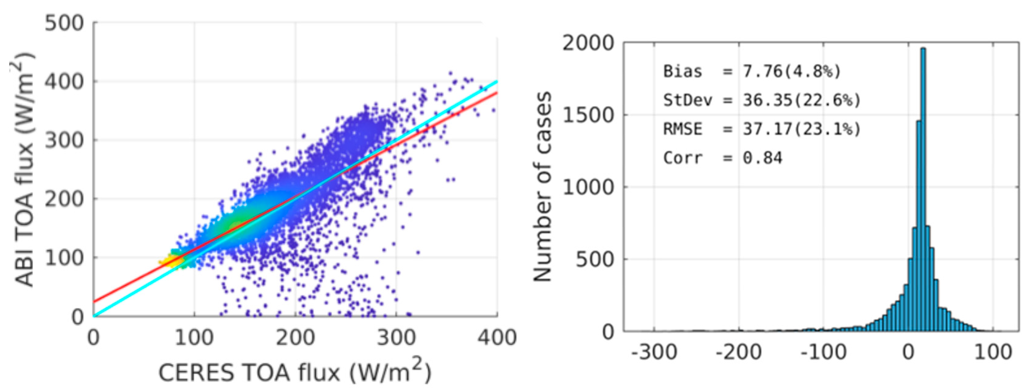
As seen in Figure 4, compared to the CERES TOA fluxes, the ABI fluxes are larger in the low range (CERES TOA fluxes less than about 100 W m-2) and smaller in the high range (CERES TOA fluxes larger than about 250 W m-2). The low and high ranges generally correspond to cloud-free scenes (and or low solar zenith angles) and cloudy (and or high solar zenith angles), respectively. In the mid-range (approximately between 100 and 250 W m-2), there is a large scatter of data points, several of them with significant negative ABI-CERES TOA flux differences. However, most of them are clustered around the one-to-one line. As a result, the frequency distribution of the ABI-CERES TOA flux differences peaks around zero with a large negative tail. Another peak at about a positive 30 W m-2 is present that comes from the low range of CERES fluxes as shown in the density scatterplot. We have conducted several experiments to identify the reason for this secondary peak.
2.5.1. Experiment 1
We applied the old approach (Pinker et al. [3]) to the ADMs and the secondary spike disappeared. The old approach is based on a synergy between the original CERES ADMs as described in Loeb et al. [6] and simulations, as described in Niu and Pinker [7]. The bias increased but there was some reduction in the standard deviation of biases.
Figure 5.
Same granule as used in Figure 4, but using the older ADM approach.
Figure 5.
Same granule as used in Figure 4, but using the older ADM approach.
2.5.2. Experiment 2
In the second experiement we have used the CERES2003 ADM for all surface types except for clear ocean. For clear ocean we replaced it with our original ADMs that combined the CERES2003 ADM models and our simulations (Niu and Pinker [7]) (hereafter Niu2011 ADM). This resulted in lower ABI fluxes in the mid range, which in turn increased the number of points below the one-to-one line and reduced the overall bias, but with practically no change in the standard deviation. (Figure 6).
2.5.3. Experiment 3
Based on the improvement seen in Experiment 2, we have redone all the cases for November 2022 using this approach (for clear ocean). The cases used are detailed in Appendix A. A summary of the results are shown in Figure 7 and detailed in Appendix B. As evident, substantial improvement has been achieved.
3. Results
3.1. Results for January, April, and July After Removing Outliers
Outliers are defined as data points with std greater than three. At least for some of the outliers, the large differences are from locations where there are only a few valid pixels available in the corresponding CERES box. In this case, the block average may not be representative of the real condition of the CERES box. The scatter plots after removing the outliers are shown below. The ADM used is the CERES2003 ADMs with ocean ADM values replaced with the old, synthesized ADMs.
Figure 8.
ABI TOA flux compared to CERES TOA flux for January 2023. The number of outliers removed was 0.7 %.
Figure 8.
ABI TOA flux compared to CERES TOA flux for January 2023. The number of outliers removed was 0.7 %.
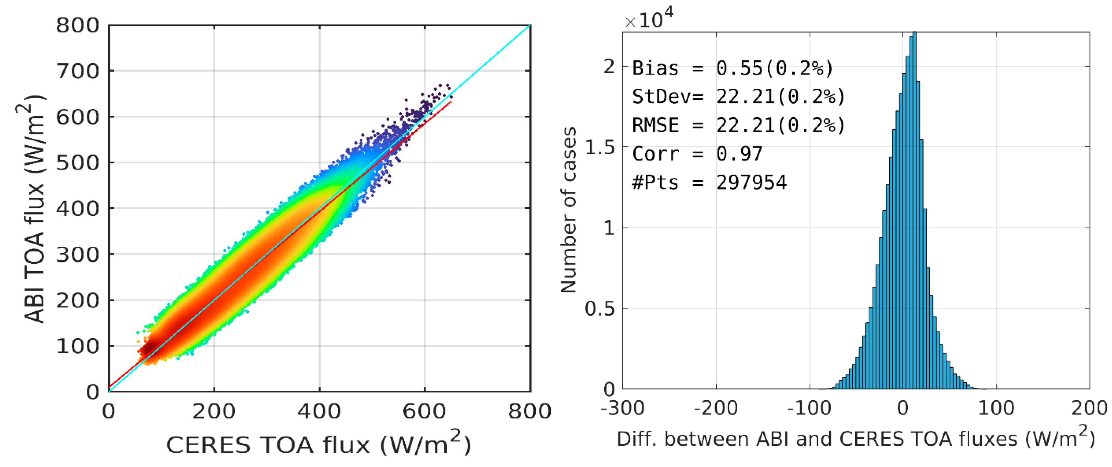
Figure 9.
ABI TOA flux compared to CERES TOA flux for April 2023. The number of outliers removed was 1 %.
Figure 9.
ABI TOA flux compared to CERES TOA flux for April 2023. The number of outliers removed was 1 %.
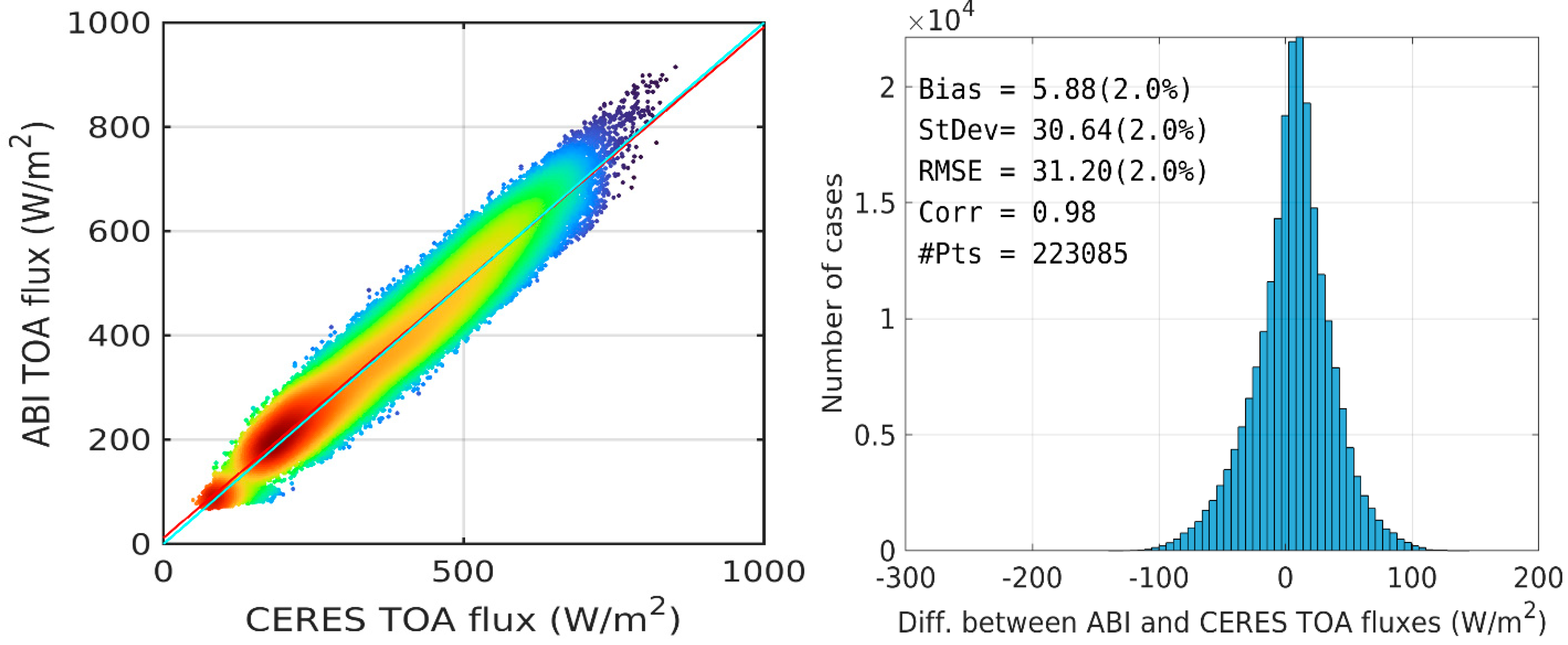
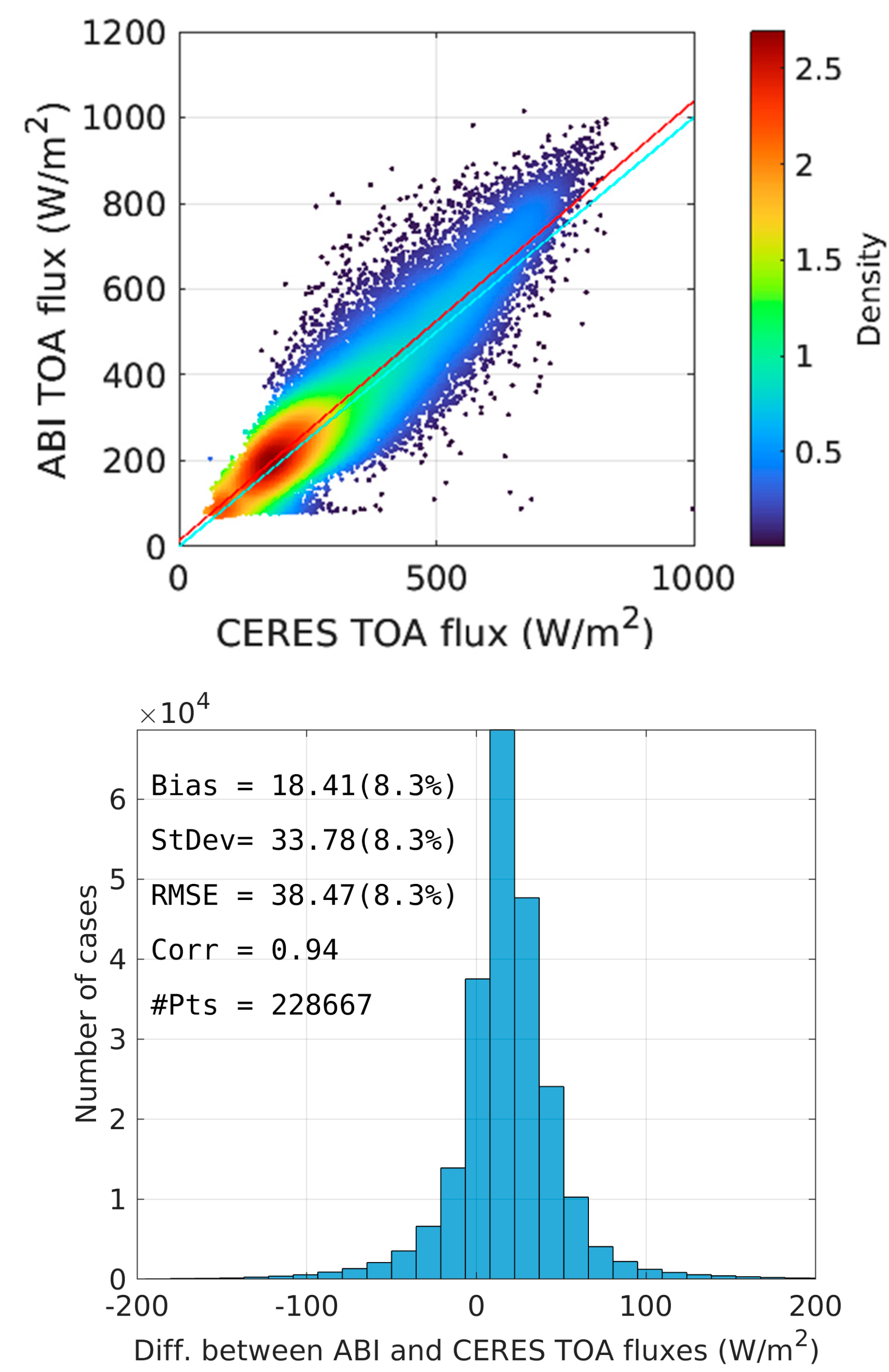
Figure 10.
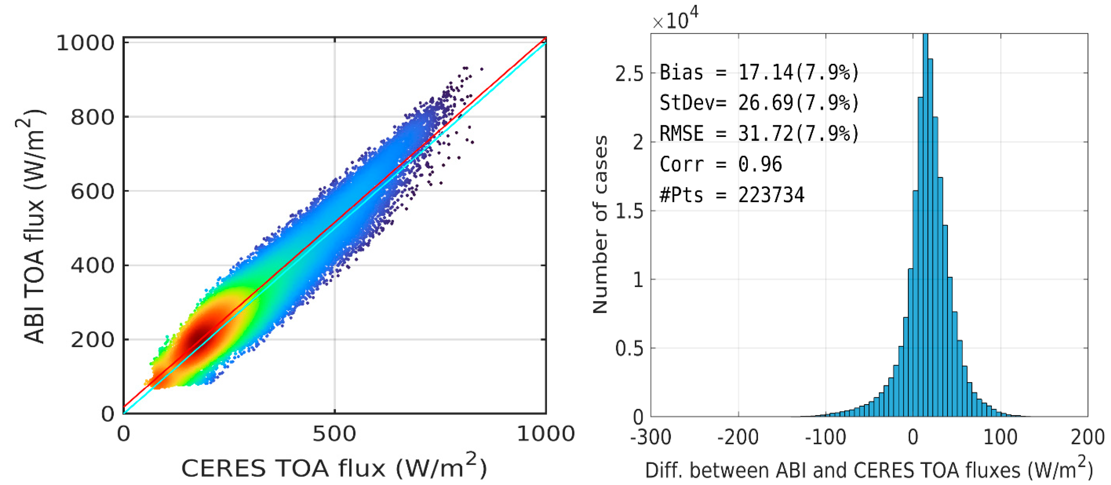
ABI TOA flux compared to CERES TOA flux for July 2023. The number of outliers removed was 2 %.
Figure 10.
ABI TOA flux compared to CERES TOA flux for July 2023. The number of outliers removed was 2 %.
3.2. Investigation of the July Case
To better understand why the results for July agree less with CERES than those for the other three months, we have investigated the cloudy conditions during the selected months. For example, we have plotted the conditions for each day for July and April 2023. We illustrate each month with one case. The notations in the following figures are:
- (a)
- Matchup between ABI and CERES swaths. Red pixels are CERES FOVs.
- (b)
- ABI flux image in 2-km resolution matched to CERES swath.
- (c)
- ABI flux image re-gridded to CERES resolution. Matched to CERES swath.
- (d)
- CERES flux image.
- (e)
- Density scatter plot between CERES and ABI.
- (f)
- Histogram and statistics.
- (g)
- ABI cloud fraction.
- (h)
- ABI 640-nm cloud optical depth.
In the following figure we illustrate the cloud conditions for 14th of July 2023. The figures show TOA fluxes that are considered as proxy for the presence of clouds Illustrated are also the results of evaluation as specified above for (a) to (f). (g) and (h) show the ABI cloud fraction and the 640-nm cloud optical depth, respectively.
It was established, and shown in Figure 11 specifically for July 14, 2023, that most July cases have clear conditions or thin clouds over the ABI-CERES overlap region. The higher bias comes mainly from the clear pixels.
We have also investigated cloud conditions during April 2023. In April, cloudy cases are more frequent than in July. A case for April is shown in Figure 12. We see a lower bias in April than in July.
4. Discussion and Summary
Most satellite observations provide information at TOA only and observe in narrow spectral bands. To derive the total flux at the TOA as well as at the surface there is a need to transform such observations into broadband fluxes. This is accomplished primarily by simulations that require validation against broadband observations. The primary source of broadband observations at the TOA comes from CERES; however, these observations also require some empirical corrections using Angular Distribution Models (ADM). As such, there is no absolute “truth” available for evaluations. In this study we use narrow-band observations from ABI on GOES-18 that are transformed to broadband based on simulations (NTB) and adjusted to total fluxes using an ADM that is a combination of the CERES2003 ADM and the Niu2011 ADM for ocean to estimate the broadband flux. Subsequently, the GOES-18 estimates are evaluated against the Clouds and the Earth's Radiant Energy System (CERES) data, the only available source of such information. The importance of agreement at the TOA is because most methodologies to derive surface SWR fluxes start with the satellite observation at the TOA. Moreover, information on radiative fluxes at both boundaries (TOA and surface) is needed for estimating the energy absorbed by the atmosphere. The methodology described to make such comparisons has been evaluated and possible sources of error were identified.
We have completed an evaluation of shortwave (SW) radiative fluxes at the top of the atmosphere (TOA) as derived from GOES-18 against CERES for four months during 2022 representing different seasons. This is the first effort to evaluate ABI for GOES-18 for such an extensive time period. In contrast to evaluation of GOES-16 and 17, we have remapped ABI observations to CERES. Previously, the mapping was from CERES to ABI. Previous experiments have shown that mapping procedures do have an impact on the results. The results of the evaluation indicate that the accuracy achieved in estimating TOA SWR fluxes ranges between 0.55 to 17.14 for the bias and 22.21 to 31.20 for the std. It is believed that the high bias of 17.14 for July is related to the predominantly clear sky conditions when the used ADMs may have some problems.
Author Contributions
The investigation and conceptualization were carried out by RTP, IL and JD. YM and WC developed the software. RTP prepared the original draft. All authors contributed to the writing, editing and review of the publication.
Competing interests
The authors declare that they have no conflict of interest.
Acknowledgments
We acknowledge the benefit from the use of the numerous data sources used in this study. These include the Clouds and the Earth's Radiant Energy System (CERES) teams, the Fast Longwave and Shortwave Radiative Flux (FLASHFlux) teams, the University of Wisconsin-Madison, Space Science and Engineering Center, Cooperative Institute for Meteorological Satellite Studies (CIMSS) for providing the SeeBor Version 5.0 data (https://cimss.ssec.wisc.edu/training_data/, and the final versions of the GOES Imager data were downloaded from https://www.bou.class.noaa.gov/. Several individuals have been involved in the early stages of the project whose contribution led to the refinement of the methodologies. These include M. M. Woncsick and Shuyan Liu.
Financial support
This research was supported by NOAA/STAR GOES-R Program under CISESS grant NA19NES4320002, award numbers RPRP_DASR_23 and RPRP_DASR_24 to the University of Maryland.
Appendix A
The list below is the GOES images that overlap with CERES Aqua and Terra satellite in November 2022. Every one of these GOES images has >10000 CERES SSFs within the GOES domain.
Match ups between ABI and CERES SSF data in 2022-11-23 00Z to 2022-12-01 23Z.
For Aqua:
OR_ABI-L1b-RadC-M6C06_G18_s20223272006173_e20223272008552_c20223272008583.nc
OR_ABI-L1b-RadC-M6C06_G18_s20223272011173_e20223272013552_c20223272013586.nc
OR_ABI-L1b-RadC-M6C06_G18_s20223272146173_e20223272148552_c20223272148582.nc
OR_ABI-L1b-RadC-M6C06_G18_s20223272151173_e20223272153552_c20223272153585.nc
OR_ABI-L1b-RadC-M6C06_G18_s20223282051175_e20223282053553_c20223282053582.nc
OR_ABI-L1b-RadC-M6C06_G18_s20223291956176_e20223291958555_c20223291958581.nc
OR_ABI-L1b-RadC-M6C06_G18_s20223292131176_e20223292133555_c20223292133582.nc
OR_ABI-L1b-RadC-M6C06_G18_s20223292136176_e20223292138555_c20223292138586.nc
OR_ABI-L1b-RadC-M6C06_G18_s20223302036177_e20223302038557_c20223302038587.nc
OR_ABI-L1b-RadC-M6C06_G18_s20223302041177_e20223302043556_c20223302043588.nc
OR_ABI-L1b-RadC-M6C06_G18_s20223311941179_e20223311943558_c20223311943588.nc
OR_ABI-L1b-RadC-M6C06_G18_s20223312121179_e20223312123558_c20223312123597.nc
OR_ABI-L1b-RadC-M6C06_G18_s20223322021170_e20223322023549_c20223322023584.nc
OR_ABI-L1b-RadC-M6C06_G18_s20223322026170_e20223322028549_c20223322028580.nc
OR_ABI-L1b-RadC-M6C06_G18_s20223332106172_e20223332108550_c20223332108584.nc
OR_ABI-L1b-RadC-M6C06_G18_s20223332111172_e20223332113550_c20223332113584.nc
OR_ABI-L1b-RadC-M6C06_G18_s20223342011173_e20223342013552_c20223342013580.nc
OR_ABI-L1b-RadC-M6C06_G18_s20223342016173_e20223342018552_c20223342018579.nc
OR_ABI-L1b-RadC-M6C06_G18_s20223342151173_e20223342153552_c20223342153580.nc
OR_ABI-L1b-RadC-M6C06_G18_s20223352051175_e20223352053553_c20223352053580.nc
OR_ABI-L1b-RadC-M6C06_G18_s20223352056175_e20223352058553_c20223352058589.nc
For Terra:
OR_ABI-L1b-RadC-M6C06_G18_s20223271801173_e20223271803552_c20223271803580.nc
OR_ABI-L1b-RadC-M6C06_G18_s20223271806173_e20223271808551_c20223271808582.nc
OR_ABI-L1b-RadC-M6C06_G18_s20223271941173_e20223271943552_c20223271943579.nc
OR_ABI-L1b-RadC-M6C06_G18_s20223271946173_e20223271948552_c20223271948584.nc
OR_ABI-L1b-RadC-M6C06_G18_s20223272121173_e20223272123552_c20223272123582.nc
OR_ABI-L1b-RadC-M6C06_G18_s20223281706174_e20223281708553_c20223281708583.nc
OR_ABI-L1b-RadC-M6C06_G18_s20223281841174_e20223281843553_c20223281843585.nc
OR_ABI-L1b-RadC-M6C06_G18_s20223281846174_e20223281848553_c20223281848583.nc
OR_ABI-L1b-RadC-M6C06_G18_s20223282021174_e20223282023553_c20223282023582.nc
OR_ABI-L1b-RadC-M6C06_G18_s20223282026174_e20223282028553_c20223282028584.nc
OR_ABI-L1b-RadC-M6C06_G18_s20223291746176_e20223291748554_c20223291748590.nc
OR_ABI-L1b-RadC-M6C06_G18_s20223291751176_e20223291753554_c20223291753582.nc
OR_ABI-L1b-RadC-M6C06_G18_s20223291926176_e20223291928555_c20223291928589.nc
OR_ABI-L1b-RadC-M6C06_G18_s20223292101176_e20223292103555_c20223292103582.nc
OR_ABI-L1b-RadC-M6C06_G18_s20223292106176_e20223292108555_c20223292108587.nc
OR_ABI-L1b-RadC-M6C06_G18_s20223301651177_e20223301653556_c20223301653585.nc
OR_ABI-L1b-RadC-M6C06_G18_s20223301826177_e20223301828556_c20223301828588.nc
OR_ABI-L1b-RadC-M6C06_G18_s20223301831177_e20223301833556_c20223301833589.nc
OR_ABI-L1b-RadC-M6C06_G18_s20223302006177_e20223302008556_c20223302008589.nc
OR_ABI-L1b-RadC-M6C06_G18_s20223302011177_e20223302013556_c20223302013584.nc
OR_ABI-L1b-RadC-M6C06_G18_s20223302146178_e20223302148556_c20223302148587.nc
OR_ABI-L1b-RadC-M6C06_G18_s20223311731179_e20223311733557_c20223311733589.nc
OR_ABI-L1b-RadC-M6C06_G18_s20223311736179_e20223311738557_c20223311738584.nc
OR_ABI-L1b-RadC-M6C06_G18_s20223311911179_e20223311913558_c20223311913585.nc
OR_ABI-L1b-RadC-M6C06_G18_s20223312046179_e20223312048558_c20223312048589.nc
OR_ABI-L1b-RadC-M6C06_G18_s20223312051179_e20223312053558_c20223312053589.nc
OR_ABI-L1b-RadC-M6C06_G18_s20223321811170_e20223321813549_c20223321813577.nc
OR_ABI-L1b-RadC-M6C06_G18_s20223321816170_e20223321818549_c20223321818578.nc
OR_ABI-L1b-RadC-M6C06_G18_s20223321951170_e20223321953549_c20223321953577.nc
OR_ABI-L1b-RadC-M6C06_G18_s20223321956170_e20223321958549_c20223321958577.nc
OR_ABI-L1b-RadC-M6C06_G18_s20223322131170_e20223322133549_c20223322133579.nc
OR_ABI-L1b-RadC-M6C06_G18_s20223331716171_e20223331718550_c20223331718578.nc
OR_ABI-L1b-RadC-M6C06_G18_s20223331851171_e20223331853550_c20223331853583.nc
OR_ABI-L1b-RadC-M6C06_G18_s20223331856171_e20223331858550_c20223331858583.nc
OR_ABI-L1b-RadC-M6C06_G18_s20223332031172_e20223332033550_c20223332033577.nc
OR_ABI-L1b-RadC-M6C06_G18_s20223332036172_e20223332038550_c20223332038587.nc
OR_ABI-L1b-RadC-M6C06_G18_s20223341756173_e20223341758552_c20223341758585.nc
OR_ABI-L1b-RadC-M6C06_G18_s20223341801173_e20223341803552_c20223341803580.nc
OR_ABI-L1b-RadC-M6C06_G18_s20223341936173_e20223341938552_c20223341938579.nc
OR_ABI-L1b-RadC-M6C06_G18_s20223342111173_e20223342113552_c20223342113582.nc
OR_ABI-L1b-RadC-M6C06_G18_s20223342116173_e20223342118552_c20223342118581.nc
OR_ABI-L1b-RadC-M6C06_G18_s20223351701174_e20223351703553_c20223351703586.nc
OR_ABI-L1b-RadC-M6C06_G18_s20223351836174_e20223351838553_c20223351838580.nc
OR_ABI-L1b-RadC-M6C06_G18_s20223351841175_e20223351843554_c20223351843586.nc
OR_ABI-L1b-RadC-M6C06_G18_s20223352016175_e20223352018554_c20223352018580.nc
OR_ABI-L1b-RadC-M6C06_G18_s20223352021175_e20223352023554_c20223352023584.nc
OR_ABI-L1b-RadC-M6C06_G18_s20223352156175_e20223352158553_c20223352158580.nc
Appendix B
Results for cases shown in Figure 7. Used is the CERES2003 ADMs except for the ocean where ADM values were replaced with the Niu2011 ADMs with number of overlapped pixels >10000. Included are the bias, standard deviation of the biases (stdev), the root mean squared error (rmserr), the percent bias (pbias), the percent standard deviation (pstd), and the correlation coefficient (corr).
bias stdev rmserr pbias* pstdev corr
________ ______ ______ ________ ______ _______
-0.85606 29.969 29.98 -0.47907 16.771 0.93384
-2.7 28.702 28.828 -1.1086 11.784 0.97182
2.181 34.005 34.073 1.0254 15.987 0.942
-12.429 39.888 41.768 -7.9541 25.526 0.76836
3.0505 28.044 28.208 1.8294 16.818 0.93876
-4.3455 34.155 34.429 -1.7507 13.76 0.95735
0.39935 37.114 37.114 0.26057 24.216 0.83205
-0.66335 29.371 29.377 -0.29131 12.898 0.96571
-0.34199 28.171 28.172 -0.13378 11.02 0.91855
-14.145 52.485 54.31 -8.8922 32.995 0.69622
6.9834 25.857 26.782 3.9258 14.536 0.95696
0.27233 28.699 28.699 0.11357 11.969 0.96866
10.119 34.905 36.34 5.0421 17.392 0.89984
-2.2489 34.614 34.684 -1.3104 20.169 0.90046
1.6483 24.734 24.788 0.76011 11.406 0.96314
5.9568 29.953 30.538 3.3553 16.871 0.92963
-3.7305 27.587 27.837 -1.7622 13.031 0.9513
5.1825 23.878 24.433 2.6886 12.388 0.96647
9.045 39.824 40.836 4.0588 17.871 0.90796
-9.4123 35.568 36.786 -4.8907 18.482 0.90337
-0.37148 25.745 25.747 -0.17625 12.215 0.95077
3.0198 31.089 31.234 1.4889 15.328 0.94944
-5.6674 30.726 31.243 -2.7831 15.089 0.93517
-7.7931 37.391 38.194 -3.6139 17.34 0.94338
10.44 27.521 29.433 4.9336 13.005 0.91576
-12.203 50.156 51.598 -7.1384 29.34 0.68105
0.89041 33.323 33.333 0.38101 14.259 0.94934
0.68753 24.821 24.83 0.34867 12.588 0.97111
-8.6732 41.674 42.564 -3.0728 14.764 0.877 -0.8863 32.7576 33.3159 -0.5223 16.5455 0.9119
*pbias is % bias
Appendix C
Detailed Statistics for each matched case for January, April and July 2023.
Table C1. January, before removing outliers.
bias stdev rmserr pbias pstdev prmserr corr numData
_________ ______ ______ _________ ______ _______ _______ _______
13.104 29.747 32.494 5.3286 12.097 13.214 0.94696 1180
0.45773 25.309 25.312 0.21162 11.701 11.702 0.97217 8985
-2.5804 20.551 20.711 -1.1447 9.1168 9.1878 0.97769 7144
-4.1269 23.16 23.524 -1.759 9.8712 10.026 0.96675 10551
-5.2965 23.058 23.655 -2.774 12.076 12.389 0.95631 4329
2.6288 24.095 24.237 1.1277 10.336 10.397 0.97184 10821
-2.1375 24.945 25.03 -1.0851 12.663 12.706 0.94767 2098
-1.3178 25.055 25.089 -0.5938 11.29 11.305 0.96471 9238
-0.66777 23.447 23.455 -0.3612 12.683 12.687 0.95339 9461
4.6342 22.732 23.199 2.1959 10.772 10.993 0.97086 11502
4.0747 24.06 24.401 1.937 11.438 11.599 0.96973 5364
1.689 23.421 23.481 0.75099 10.414 10.44 0.97376 12566
3.2493 23.902 24.118 1.5377 11.312 11.414 0.96506 3170
6.1204 25.909 26.62 2.5249 10.688 10.982 0.97358 8994
1.7406 24.585 24.645 0.89419 12.63 12.661 0.94372 8858
12.101 23.417 26.35 5.6804 10.992 12.369 0.95341 1183
6.3615 22.22 23.112 2.9713 10.378 10.795 0.97387 11787
10.007 24.525 26.487 4.2734 10.473 11.311 0.96856 14155
12.29 27.712 30.282 5.1862 11.694 12.778 0.91189 385
-0.032878 23.466 23.465 -0.012176 8.6902 8.6898 0.9728 10250
5.564 24.483 25.104 1.8739 8.2457 8.4549 0.9623 3968
0.6974 19.425 19.436 0.30349 8.4531 8.4582 0.98226 10953
-0.47176 23.426 23.426 -0.19619 9.7419 9.7417 0.9675 2241
-0.69884 25.326 25.334 -0.32141 11.648 11.652 0.96292 11247
-4.4586 23.092 23.518 -2.0541 10.639 10.835 0.96674 9932
7.7451 26.655 27.743 3.376 11.619 12.093 0.95598 866
-1.74 24.196 24.257 -0.84576 11.761 11.791 0.97138 11245
-6.7573 18.636 19.821 -3.325 9.1698 9.7532 0.97581 5812
0.32497 19.679 19.681 0.15 9.0839 9.0848 0.98479 12741
-2.1467 23.768 23.861 -0.87605 9.6994 9.7376 0.96599 3622
-2.6019 21.027 21.186 -1.242 10.037 10.113 0.97631 9266
-0.099278 22.266 22.26 -0.042418 9.5136 9.511 0.9634 1760
7.7764 19.779 21.251 3.9528 10.054 10.802 0.98055 8305
1.3074 22.653 22.69 0.55848 9.6771 9.6926 0.97328 8123
1.8388 21.974 22.049 0.81621 9.7535 9.7871 0.98052 10360
-0.21369 26.299 26.298 -0.082323 10.131 10.131 0.96942 5477
-10.653 24.022 26.277 -4.473 10.087 11.033 0.97197 11298
-7.7988 26.764 27.872 -3.061 10.505 10.94 0.94241 2586
-0.24185 27.161 27.16 -0.12118 13.609 13.609 0.96506 8660
-5.387 24.828 25.405 -2.2953 10.579 10.824 0.97326 10582
Table C2. January, after removing outliers.
bias stdev rmserr pbias pstdev prmserr corr numData
________ ______ ______ _________ ______ _______ _______ _______
11.614 27.119 29.491 4.7702 11.139 12.113 0.95504 1159
0.76158 22.324 22.336 0.35456 10.393 10.399 0.97802 8854
-2.9547 19.014 19.241 -1.3158 8.4674 8.5685 0.98087 7077
-3.4773 21.203 21.486 -1.4842 9.0504 9.1708 0.97204 10421
-5.2156 21.151 21.783 -2.7439 11.128 11.46 0.96269 4286
2.6296 22.926 23.075 1.1291 9.8444 9.9085 0.9745 10756
-2.3914 23.76 23.875 -1.2182 12.103 12.161 0.95195 2081
-0.90303 23.804 23.82 -0.4068 10.723 10.73 0.96848 9178
-0.74913 21.536 21.548 -0.40716 11.705 11.711 0.96045 9361
4.7698 21.13 21.661 2.2645 10.032 10.284 0.97508 11374
3.477 21.6 21.876 1.6658 10.348 10.48 0.97498 5283
1.4145 21.74 21.785 0.63085 9.6959 9.716 0.97737 12432
2.5599 22.453 22.595 1.2143 10.651 10.718 0.96942 3141
5.9148 25.238 25.92 2.4428 10.423 10.705 0.97518 8958
2.2825 22.469 22.583 1.1774 11.59 11.649 0.95127 8761
11.707 22.918 25.727 5.5106 10.788 12.11 0.95513 1176
5.8713 21.156 21.955 2.7488 9.9047 10.279 0.97648 11675
9.1296 22.549 24.327 3.9203 9.6827 10.446 0.97337 13932
11.645 26.827 29.213 4.9244 11.345 12.354 0.91793 382
-0.30366 22.34 22.341 -0.11266 8.2882 8.2885 0.97525 10165
5.1824 22.686 23.268 1.7469 7.6473 7.8433 0.96777 3925
0.93588 17.959 17.983 0.408 7.8294 7.8397 0.98486 10836
-0.60629 21.886 21.89 -0.2522 9.1042 9.1056 0.97209 2219
-0.35978 24.083 24.084 -0.16577 11.096 11.097 0.96643 11155
-3.6073 21.036 21.342 -1.6618 9.6908 9.8317 0.97236 9818
7.4053 25.138 26.192 3.2396 10.997 11.458 0.96112 856
-1.2546 22.046 22.081 -0.61213 10.756 10.773 0.97633 11148
-6.2106 17.165 18.253 -3.059 8.4546 8.9903 0.9796 5751
0.73326 18.633 18.647 0.33931 8.6223 8.6286 0.98632 12639
-2.0976 22.591 22.685 -0.85622 9.2214 9.2598 0.96951 3593
-2.2509 19.567 19.695 -1.0777 9.3678 9.4291 0.9794 9172
-0.20512 20.211 20.207 -0.087581 8.6298 8.6277 0.97007 1735
8.4614 17.614 19.54 4.3119 8.976 9.9575 0.9845 8217
1.0203 20.95 20.974 0.43742 8.9816 8.9917 0.97706 8037
1.9711 19.681 19.779 0.87726 8.7591 8.8025 0.98459 10238
-0.31496 23.435 23.434 -0.12177 9.0602 9.0602 0.97553 5389
-10.025 22.584 24.708 -4.2158 9.4968 10.39 0.9753 11163
-7.7282 25.605 26.741 -3.0347 10.054 10.5 0.94724 2568
-0.40962 24.71 24.712 -0.20687 12.479 12.48 0.97087 8537
-5.3007 23.663 24.248 -2.2613 10.095 10.344 0.97579 10506
Table C3. April, before removing outliers.
bias stdev rmserr pbias pstdev prmserr corr numData
_______ ______ ______ ________ ______ _______ _______ _______
6.3927 32.54 33.161 2.0463 10.416 10.615 0.97869 13803
10.549 33.554 35.165 3.5387 11.256 11.796 0.9779 1906
8.7018 35.279 36.333 2.3276 9.4366 9.7186 0.97124 5346
5.2881 35.438 35.828 1.4071 9.4299 9.5336 0.98048 6976
-7.1726 36.432 37.129 -2.0231 10.276 10.472 0.98021 7656
-9.2121 33.955 35.179 -2.7715 10.215 10.584 0.97916 5023
-2.2479 29.31 29.394 -0.81003 10.562 10.592 0.98207 8921
4.1096 42.149 42.345 1.3431 13.776 13.839 0.95446 4816
-1.0489 37.602 37.612 -0.27951 10.02 10.023 0.9681 4669
6.0913 31.8 32.376 1.9959 10.42 10.609 0.97021 7534
14.012 33.614 36.405 5.343 12.817 13.881 0.95442 1186
12.612 29.678 32.245 4.4593 10.493 11.401 0.98153 7358
10.648 33.167 34.832 4.0319 12.558 13.189 0.96645 6445
14.713 29.905 33.327 5.0249 10.214 11.382 0.97588 7823
12.055 42.911 44.566 4.1201 14.666 15.232 0.93814 3647
10.795 36.486 38.047 2.879 9.731 10.147 0.97819 7805
9.1791 43.425 44.374 2.3281 11.014 11.255 0.97056 1999
8.8867 35.077 36.182 3.101 12.24 12.626 0.96343 5620
4.3037 28.102 28.428 1.6294 10.64 10.763 0.97121 7122
3.4387 20.621 20.891 1.7495 10.491 10.629 0.91169 719
9.2589 28.242 29.719 3.2688 9.9707 10.492 0.97567 7072
9.2641 32.509 33.8 3.8185 13.399 13.931 0.93371 5002
9.8469 37.58 38.846 2.8431 10.85 11.216 0.97455 7916
14.012 37.974 40.47 4.1579 11.268 12.009 0.97914 2999
2.7628 34.025 34.135 0.98996 12.192 12.231 0.97989 6002
3.7853 30.076 30.312 1.3343 10.602 10.685 0.98208 9373
0.66747 43.915 43.902 0.17523 11.529 11.526 0.95689 1238
5.2542 30.074 30.528 1.9433 11.123 11.291 0.98726 9744
-4.8184 33.678 34.019 -1.7026 11.9 12.021 0.97178 6646
6.4544 29.791 30.48 2.1917 10.116 10.35 0.97196 7348
2.8646 36.358 36.466 1.094 13.885 13.926 0.93823 3671
9.4512 34.751 36.011 3.0855 11.345 11.756 0.97421 7699
4.8481 36.47 36.782 1.9396 14.591 14.716 0.94603 2056
9.6587 30.278 31.779 3.7656 11.804 12.389 0.9691 5380
8.2933 36.907 37.825 2.6168 11.645 11.935 0.97417 6824
-11.632 48.193 49.547 -4.0388 16.733 17.203 0.91001 768
12.053 24.804 27.576 5.5133 11.346 12.614 0.94872 7105
5.0914 25.303 25.808 2.3969 11.912 12.15 0.90191 5158
10.944 24.307 26.656 4.71 10.461 11.472 0.95212 7544
Table C4. April, after removing outliers.
bias stdev rmserr pbias pstdev prmserr corr numData
________ ______ ______ ________ ______ _______ _______ _______
5.7429 30.536 31.07 1.8459 9.8147 9.9864 0.98122 13663
9.4321 30.652 32.062 3.2006 10.401 10.88 0.98105 1876
8.3125 33.613 34.622 2.2284 9.011 9.2816 0.97386 5309
5.3388 33.843 34.259 1.424 9.0266 9.1376 0.98218 6925
-5.4702 31.327 31.799 -1.5565 8.9142 9.0485 0.98525 7483
-8.0037 29.744 30.799 -2.4374 9.0582 9.3795 0.98324 4915
-1.0365 26.137 26.156 -0.37776 9.5258 9.5327 0.98501 8777
1.5724 34.7 34.732 0.51883 11.45 11.46 0.96922 4728
-0.91641 36.947 36.954 -0.24419 9.8448 9.8468 0.96928 4652
5.6348 29.836 30.361 1.8559 9.8268 9.9999 0.97349 7457
12.261 30.623 32.974 4.7278 11.808 12.715 0.9614 1164
12.129 27.753 30.286 4.3135 9.8697 10.771 0.98378 7282
8.7449 27.586 28.937 3.3768 10.652 11.174 0.97409 6314
14.089 27.333 30.749 4.848 9.405 10.58 0.97953 7710
9.1851 36.221 37.362 3.1936 12.594 12.991 0.95232 3572
10.013 34.207 35.641 2.6841 9.1692 9.5534 0.98069 7718
9.0734 41.881 42.842 2.3042 10.636 10.88 0.97259 1986
7.9169 30.833 31.831 2.7927 10.877 11.229 0.97096 5537
4.1334 26.627 26.944 1.5723 10.129 10.249 0.97384 7062
2.8696 16.602 16.837 1.4796 8.5601 8.681 0.93256 702
9.218 26.644 28.192 3.268 9.4459 9.9946 0.97821 7009
8.2833 28.202 29.39 3.4669 11.804 12.301 0.9432 4916
8.5062 33.941 34.988 2.4763 9.8805 10.185 0.97878 7814
13.531 36.142 38.586 4.034 10.775 11.503 0.98109 2971
3.0375 31.887 32.029 1.0955 11.501 11.552 0.98224 5943
3.6122 28.815 29.039 1.2802 10.212 10.292 0.98343 9306
1.1295 41.378 41.377 0.29675 10.872 10.871 0.96155 1227
5.8719 27.047 27.675 2.1909 10.092 10.326 0.98962 9618
-4.3313 31.925 32.215 -1.5344 11.31 11.413 0.97462 6589
6.0352 28.206 28.842 2.0615 9.6343 9.8518 0.97446 7284
2.6655 33.312 33.414 1.0255 12.816 12.856 0.94687 3623
8.7521 31.852 33.031 2.8916 10.524 10.913 0.97745 7600
4.0008 33.008 33.242 1.6157 13.33 13.425 0.95499 2026
9.6682 27.666 29.305 3.7885 10.841 11.483 0.97387 5324
7.6656 34.233 35.078 2.4391 10.893 11.162 0.97713 6749
-11.81 44.588 46.097 -4.1109 15.521 16.046 0.92294 760
11.907 22.435 25.398 5.5014 10.366 11.735 0.95468 7013
5.9755 22.021 22.816 2.8328 10.439 10.816 0.919 5068
10.655 21.083 23.621 4.6407 9.1826 10.288 0.95974 7413
Table C5. July, before removing outliers.
bias stdev rmserr pbias pstdev prmserr corr numData
______ ______ ______ ______ ______ _______ _______ _______
20.694 26.243 33.42 10.155 12.878 16.4 0.90539 13375
17.396 24.854 30.33 9.0184 12.885 15.724 0.81099 1450
17.382 19.077 25.808 9.3403 10.251 13.868 0.94612 6854
17.248 38.868 42.521 7.0655 15.922 17.418 0.94271 6318
17.529 36.218 40.235 6.443 13.312 14.789 0.96597 7337
17.207 41.83 45.226 6.8164 16.57 17.916 0.9485 4223
16.589 41.72 44.895 6.8884 17.323 18.642 0.90333 7862
23.884 32.594 40.405 10.976 14.979 18.568 0.81538 3572
19.274 35.886 40.732 8.0807 15.045 17.077 0.91874 5104
18.971 28.491 34.228 8.4596 12.705 15.263 0.93202 7147
22.126 19.027 29.174 11.552 9.9338 15.232 0.8025 781
20.068 30.156 36.221 9.332 14.023 16.844 0.89747 7288
14.39 46.41 48.586 6.1757 19.917 20.851 0.89749 5674
21.455 35.36 41.358 8.1797 13.481 15.768 0.97334 8574
19.231 29.835 35.491 8.263 12.819 15.25 0.95823 2982
15.832 32.787 36.407 7.1771 14.864 16.505 0.91656 8194
36.126 38.139 52.524 16.093 16.989 23.397 0.8766 1460
19.98 23.786 31.063 9.5173 11.33 14.796 0.9216 6547
25.967 31.113 40.523 11.63 13.935 18.149 0.9173 6748
17.488 26.36 31.632 8.1182 12.237 14.684 0.93755 7575
21.096 45.586 50.226 8.9341 19.305 21.27 0.92596 4002
16.241 35.764 39.277 7.4357 16.374 17.983 0.94511 9544
17.692 35.198 39.386 6.9747 13.876 15.527 0.95725 1913
22.353 26.665 34.793 10.743 12.815 16.721 0.95804 5637
20.527 30.693 36.923 8.8063 13.168 15.841 0.96823 7738
18.071 18.083 25.556 9.2799 9.2858 13.124 0.85266 748
21.258 23.13 31.414 10.283 11.188 15.195 0.90377 7194
16.486 34.036 37.815 7.6338 15.76 17.51 0.90779 5015
17.992 33.435 37.967 7.9986 14.864 16.879 0.96283 8741
14.22 42.866 45.156 6.5271 19.675 20.727 0.8926 3123
17.346 31.992 36.39 7.7389 14.273 16.235 0.9334 8265
18.95 34.228 39.122 9.914 17.907 20.467 0.93652 8263
15.842 41.009 43.959 6.4923 16.806 18.015 0.93568 6021
16.998 30.122 34.586 8.2244 14.574 16.734 0.96407 9760
10.441 38.427 39.816 4.6305 17.042 17.658 0.90742 4045
14.949 42.506 45.056 6.3811 18.145 19.233 0.94592 8930
16.466 41.38 44.526 7.1613 17.996 19.365 0.91668 2006
16.462 31.506 35.546 9.169 17.548 19.798 0.96213 8657
Table C6. July, after removing outliers.
bias stdev rmserr pbias pstdev prmserr corr numData
______ ______ ______ ______ ______ _______ _______ _______
20.162 17.694 26.825 10.058 8.827 13.382 0.94183 13157
15.538 19.346 24.808 8.2128 10.225 13.112 0.83343 1406
16.147 15.84 22.619 8.8078 8.64 12.338 0.95758 6680
16.284 29.022 33.276 6.8307 12.174 13.958 0.96273 6187
15.951 30.023 33.995 6.0162 11.324 12.822 0.97314 7198
17.101 35.894 39.756 6.8684 14.416 15.967 0.96034 4149
15.806 31.638 35.365 6.704 13.419 14.999 0.92942 7693
22.038 27.934 35.578 10.271 13.018 16.581 0.82959 3507
17.824 28.223 33.378 7.6048 12.042 14.241 0.94312 5001
18.692 24.104 30.501 8.4616 10.912 13.807 0.93977 7023
19.399 15.046 24.544 10.334 8.0148 13.074 0.79435 740
18.939 23.247 29.984 8.9751 11.016 14.209 0.9253 7123
12.903 37.593 39.743 5.6825 16.556 17.502 0.92159 5545
19.203 28.49 34.356 7.5994 11.275 13.596 0.97827 8320
17.535 24.869 30.426 7.6788 10.891 13.324 0.96665 2925
16.124 26.863 31.329 7.3912 12.314 14.361 0.93679 8044
35.314 36.139 50.519 15.873 16.244 22.708 0.88008 1444
19.155 20.585 28.118 9.2091 9.8966 13.518 0.93346 6448
24.749 28.397 37.667 11.234 12.89 17.098 0.92199 6615
16.299 22.253 27.582 7.7269 10.549 13.076 0.93617 7441
18.47 34.259 38.917 8.1598 15.135 17.193 0.93916 3884
16.353 27.256 31.784 7.6126 12.688 14.796 0.96403 9391
17.826 28.326 33.462 7.1407 11.347 13.404 0.96973 1869
20.685 20.199 28.91 10.251 10.01 14.327 0.96591 5501
19.125 24.261 30.892 8.5313 10.823 13.78 0.97116 7559
17.864 14.455 22.974 9.2828 7.5113 11.938 0.87414 728
20.179 19.641 28.158 9.8831 9.6196 13.791 0.91472 7051
15.58 25.327 29.733 7.4048 12.038 14.132 0.93112 4898
15.246 26.609 30.666 7.119 12.425 14.319 0.9637 8480
12.084 34.548 36.595 5.7036 16.307 17.273 0.91312 3047
16.784 26.36 31.249 7.6477 12.011 14.238 0.94342 8107
16.226 22.013 27.345 8.822 11.968 14.868 0.95987 8084
14.094 31.501 34.508 5.9873 13.382 14.66 0.94835 5862
15.628 23.58 28.288 7.7619 11.711 14.049 0.97361 9576
10.106 33.318 34.813 4.5379 14.96 15.631 0.92451 3982
12.974 33.189 35.633 5.7596 14.733 15.818 0.95523 8686
15.296 33.682 36.985 6.7889 14.949 16.415 0.93892 1963
13.767 19.637 23.981 8.169 11.652 14.23 0.97366 8420
Appendix D
Results for January, April, and July using all available observations
Figure D1.
ABI TOA flux compared to CERES TOA flux for January 2023.
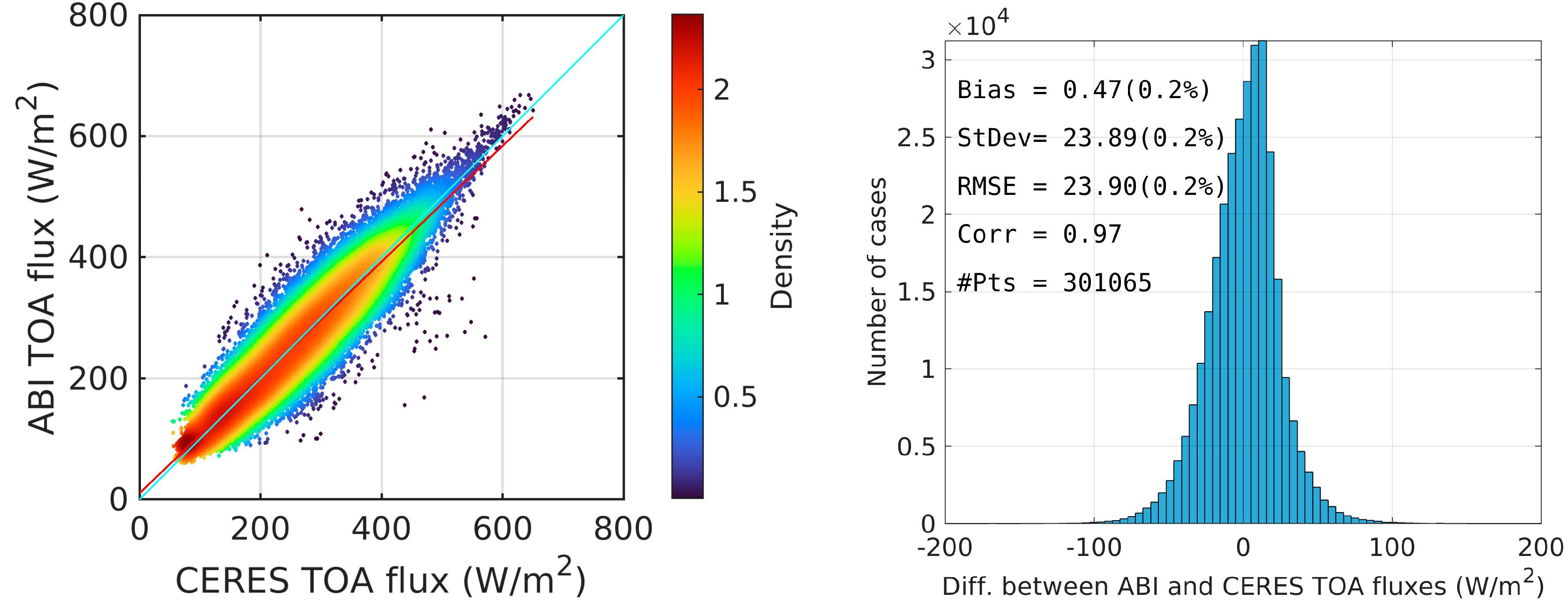
Figure D2.
ABI TOA flux compared to CERES TOA flux for April 2023.
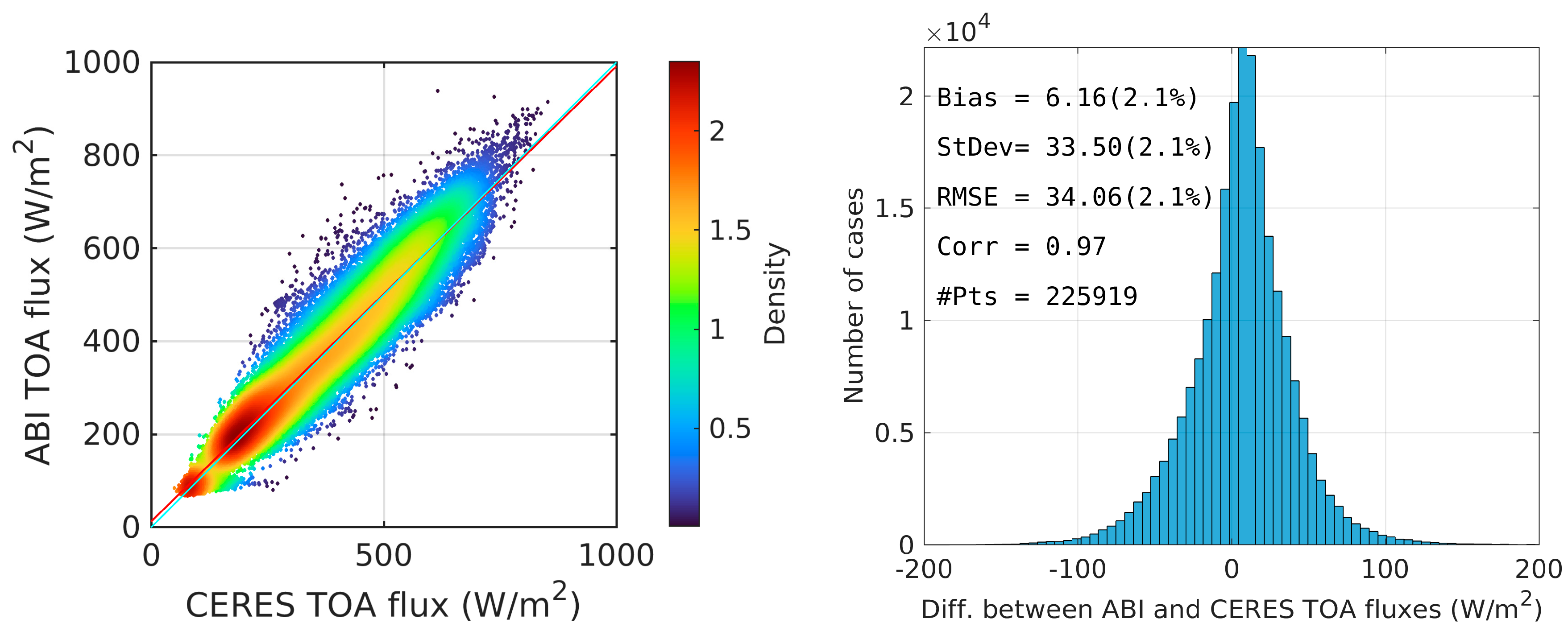
Figure D3.
ABI TOA flux compared to CERES TOA flux for July 2023.
References
- Laszlo, I.; Liu, H.; Kim, H.-Y.; Pinker, R.T. GOES-R Advanced Baseline Imager (ABI) Algorithm Theoretical Basis Document (ATBD) for Downward Shortwave Radiation (Surface), and Reflected Shortwave Radiation (TOA), version 3.1. 2018. Available online: https://www.goes-r.gov/resources/docs.html.
- Laszlo, I.; Liu, H.; Kim, H.-Y.; Pinker, R.T. (2020). Shortwave Radiation from ABI on the GOES-R Series, in The GOES-R Series, edited by S. J. Goodman, T. J. Schmit, J. Daniels and R. J. Redmon, pp. 179-191, Elsevier. [CrossRef]
- Pinker, R.T.; Ma, Y.; Chen, W.; Laszlo, I.; Liu, H.; Kim, H.-K.; Daniels, J. Top of the Atmosphere Reflected Shortwave Radiative Fluxes from GOES R. Atmos. Meas. Tech. 2022, 15, 5077–5094. [Google Scholar] [CrossRef]
- Berk et al 1998 MODTRANCloud Multiple Scattering Upgrades with Application to, A. V.I.R.I.S. Berk et al. (1998). MODTRAN Cloud and Multiple Scattering Upgrades with Application to AVIRIS. Remote Sensing of Environment 1998, 65, 367–375. [Google Scholar] [CrossRef]
- Hansen, M.C.; Defries, R.S.; Townshend, J.R.G.; Sohlberg, R. Global land cover classification at 1km spatial resolution using a classification tree approach, Int. J. Remote Sens. 2010, 21, 1331–1364. [Google Scholar] [CrossRef]
- Loeb, N.G.; Smith, N.M.; Kato, S.; Miller, W.F.; Gupta, S.K.; Minnis, P.; Wielicki, B.A. Angular Distribution Models for Top-of Atmosphere Radiative Flux Estimation from the Mission Satellite, Part I: Methodology. J. Appl. Meteorol. 2003, 42, 240–265. [Google Scholar] [CrossRef]
- Niu, X.; Pinker, R. T. Revisiting satellite radiative flux computations at the top of the atmosphere, International Journal of Remote Sensing 2011. [CrossRef]
- Loveland, T.R.; Reed, B.C.; Brown, J.F.; Ohlen, D.O.; Zhu, Z.; Yang, L.; Merchant, J.W. Development of a global land cover characteristics database and IGBP DISCover from 1 km AVHRR data, Int. J. Remote Sens. 2010, 21, 1303–1330. [Google Scholar] [CrossRef]
- Su, W.; Corbett, J.; Eitzen, Z.; Liang, L. Next-generation angular distribution models for top-of-atmosphere radiative flux calculation from CERES instruments: Methodology, 2015. Atmos. Meas. Tech. 2015, 8, 611–632. [Google Scholar] [CrossRef]
- Su, W.; Corbett, J.; Eitzen, Z.; Liang, L. Next-generation angular distribution models for top-of-atmosphere radiative flux calculation from CERES instruments: Validation, 2015. Atmos. Meas. Tech. 2015, 8, 3297–3313. [Google Scholar] [CrossRef]
Figure 1.
Illustration of the Pacific U.S. (PACUS) sector coverage of the GOES-West (currently, GOES-18) satellite.
Figure 1.
Illustration of the Pacific U.S. (PACUS) sector coverage of the GOES-West (currently, GOES-18) satellite.
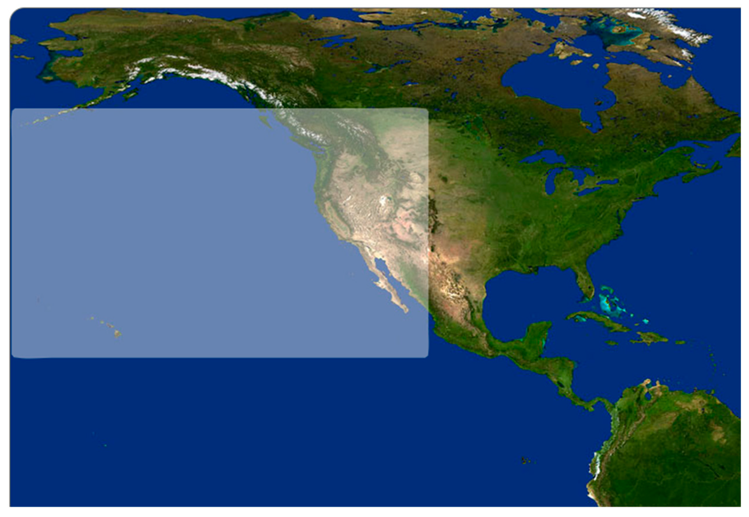
Figure 2.
An example of matchup between CERES and ABI for day 327 in 2022, 21:21:17 UTC. The blue background is the ABI TOA radiative flux, and the magenta indicates the CERES pixels that overlap with the ABI.
Figure 2.
An example of matchup between CERES and ABI for day 327 in 2022, 21:21:17 UTC. The blue background is the ABI TOA radiative flux, and the magenta indicates the CERES pixels that overlap with the ABI.
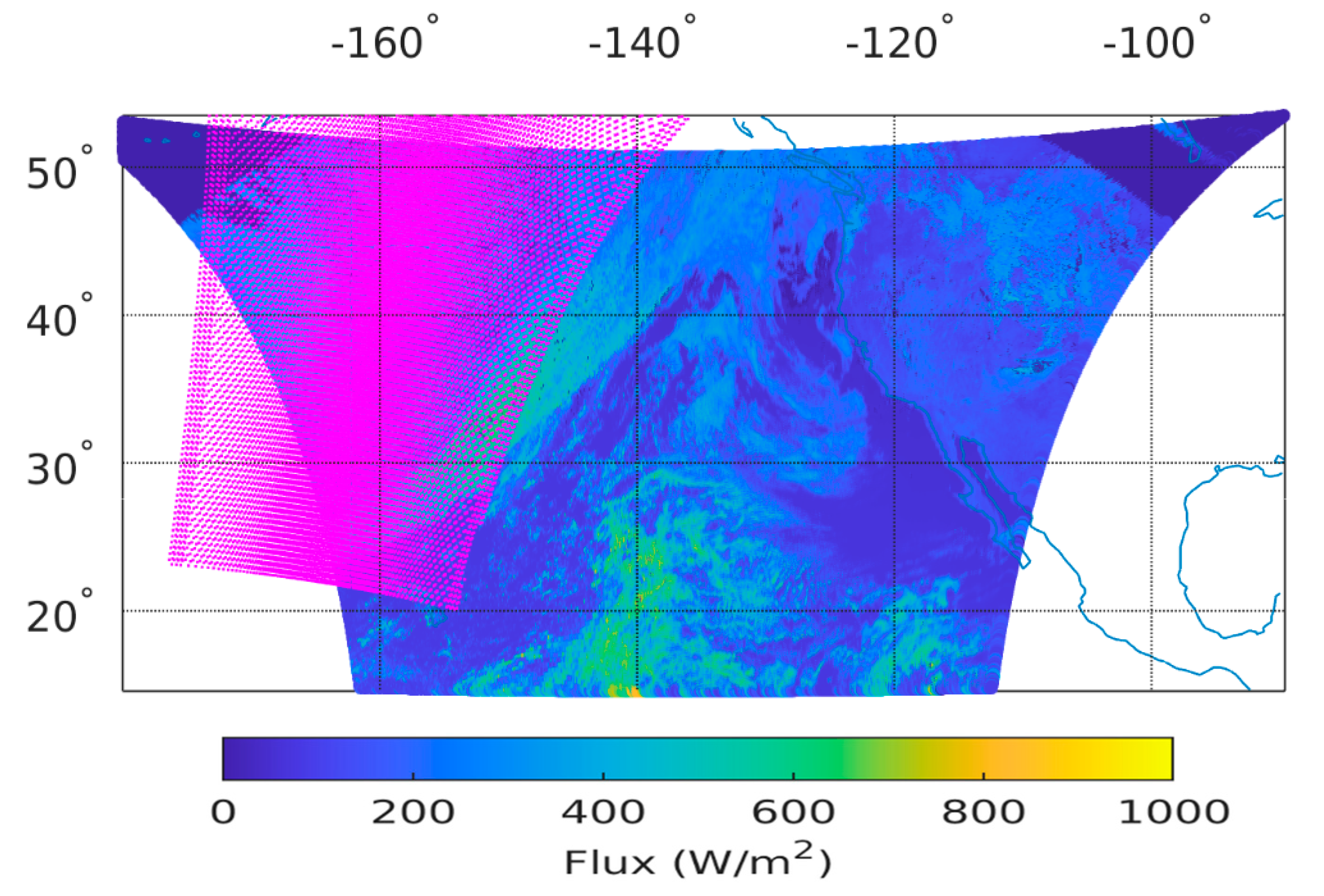
Figure 3.
(a): An example of finding CERES pixels that fall within the ABI domain around 2022 12 1, 17:15:00 UTC. x, y axis are ABI CONUS image column and row number (out of 1500 x 2500). Each point represents the center of a single CERES SSF footprint. (b): Average of ABI data to match the CERES SSF data. Panel (b) is for the same time as that for (a). The small white rectangles show the center location of 10 CERES pixels. The green block is a 16x32 km block of ABI data centered on a CERES pixel.
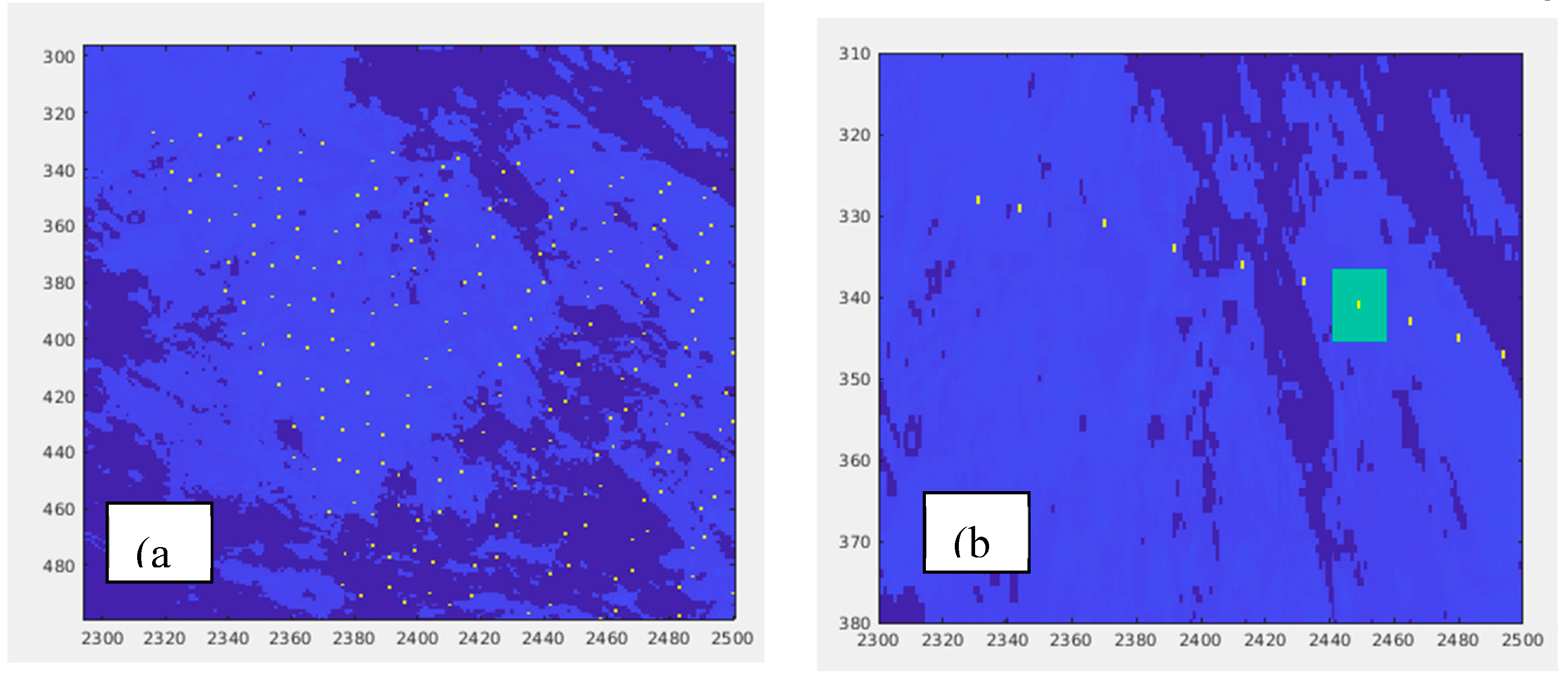
Figure 4.
Results for a single granule for year 2022 day 329 at 17:46 UTC using the CERES2003 ADM. Density scatterplot of ABI vs. CERES TOA fluxes (left), and histogram of ABI-CERES differences (right). In the density scatter plot, the solid red line is the linear fit line, and the light blue line is the one-to-one line.

Figure 6.
Here we use CERES2003 ADMs except for the clear ocean where ADM values are replaced with the old, combined ADMs (Niu2011 ADM); same cases as used previously.
Figure 6.
Here we use CERES2003 ADMs except for the clear ocean where ADM values are replaced with the old, combined ADMs (Niu2011 ADM); same cases as used previously.
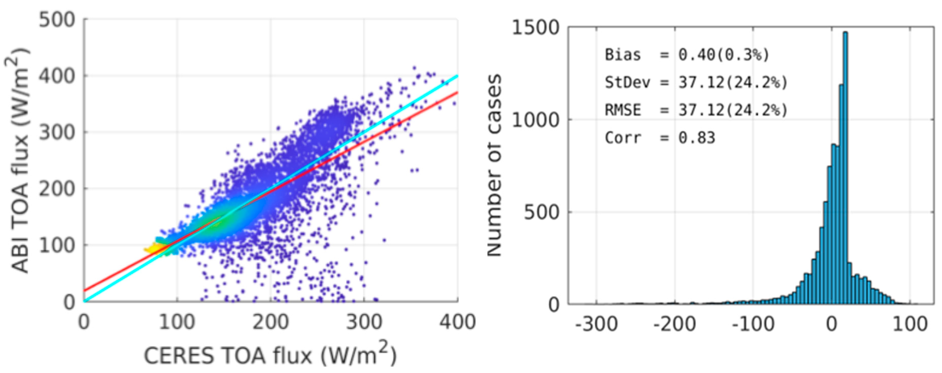
Figure 7.
These results are for November 2022 using all the cases listed in Appendix A. The ADM used is CERES2003 ADMs except for the ocean where ADM values are replaced with the old, synthesized ADMs.
Figure 7.
These results are for November 2022 using all the cases listed in Appendix A. The ADM used is CERES2003 ADMs except for the ocean where ADM values are replaced with the old, synthesized ADMs.
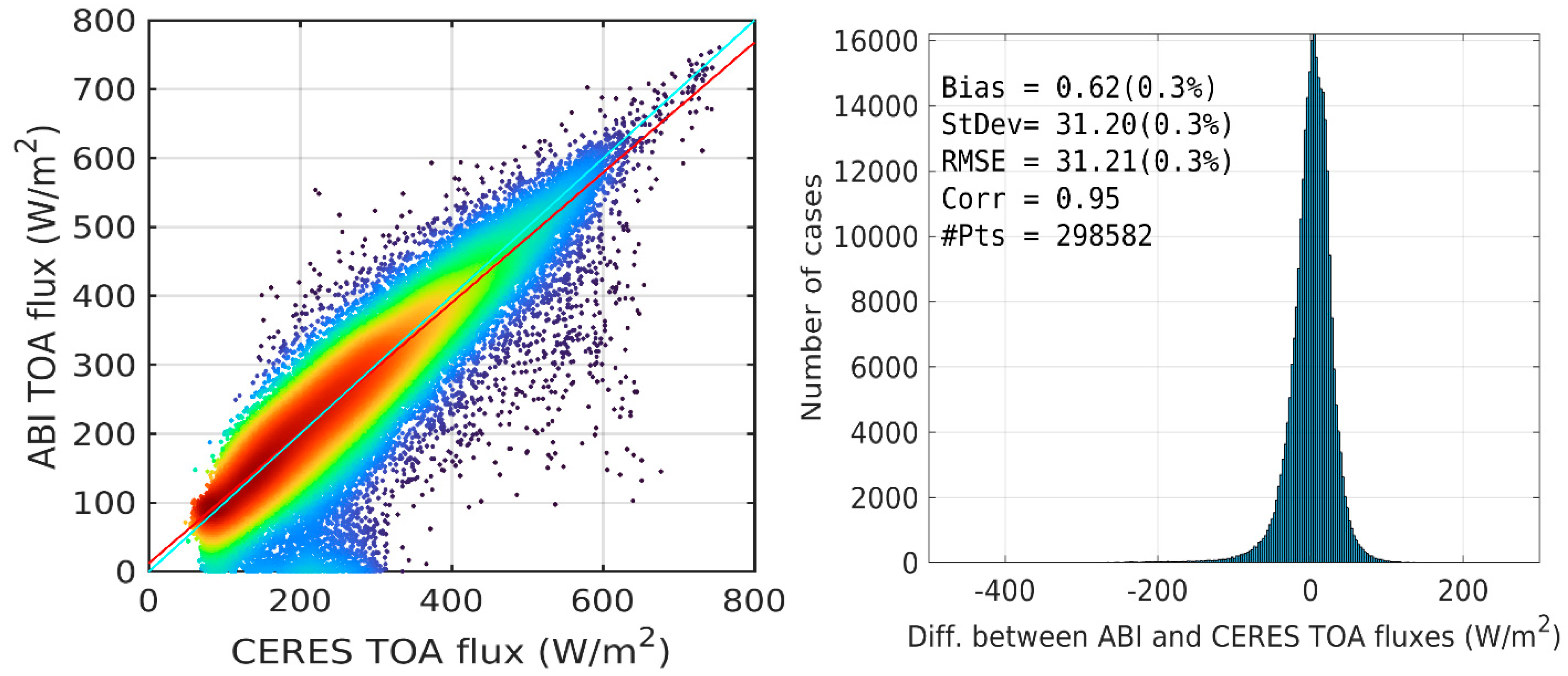
Figure 11.
The cloud conditions during 14th of July 2023, 18:31:18 UTC and relevant results of evaluation. (a) Matchup between ABI and CERES swaths. Red pixels are CERES FOVs. (b) 2-km ABI flux matched to the CERES swath. (c) ABI flux matched to the CERES swath and re-gridded to CERES resolution. (d) CERES flux. (e) Density scatter plot between CERES and ABI. (f) Histogram and statistics. (g) ABI cloud fraction. (h) ABI 640-nm cloud optical depth. The region within the white dashed lines in (g) and (h) marks the approximate area of CERES observations.
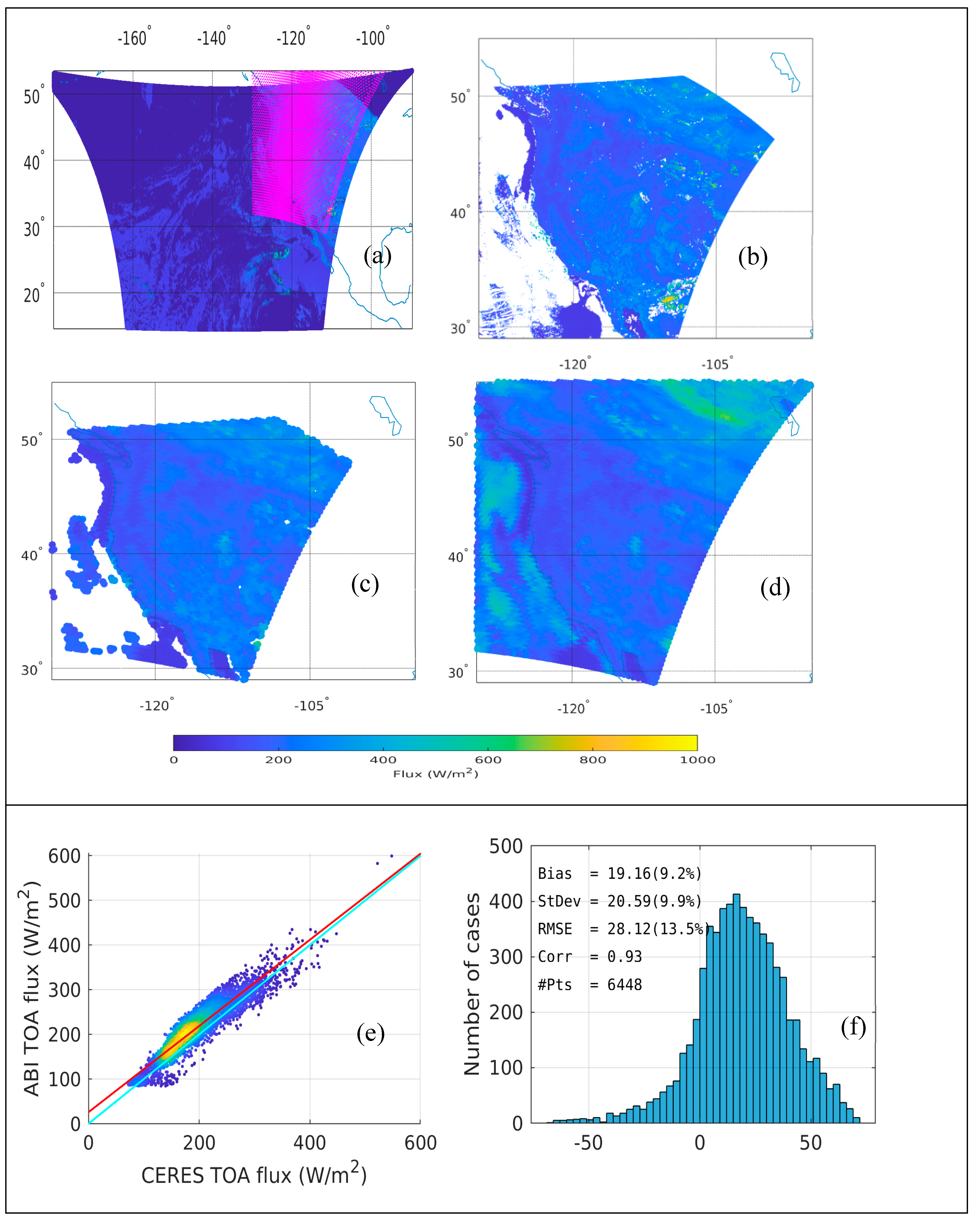
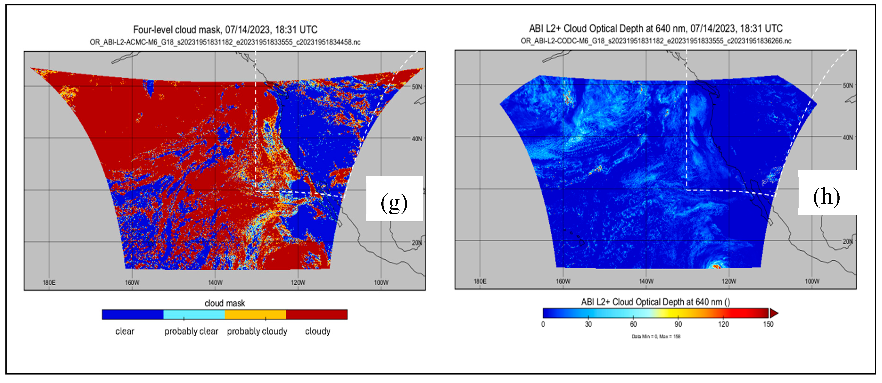
Figure 12.
Same as Figure 11 but for April 4, 2023, 18:26:17 UTC.
Figure 12.
Same as Figure 11 but for April 4, 2023, 18:26:17 UTC.
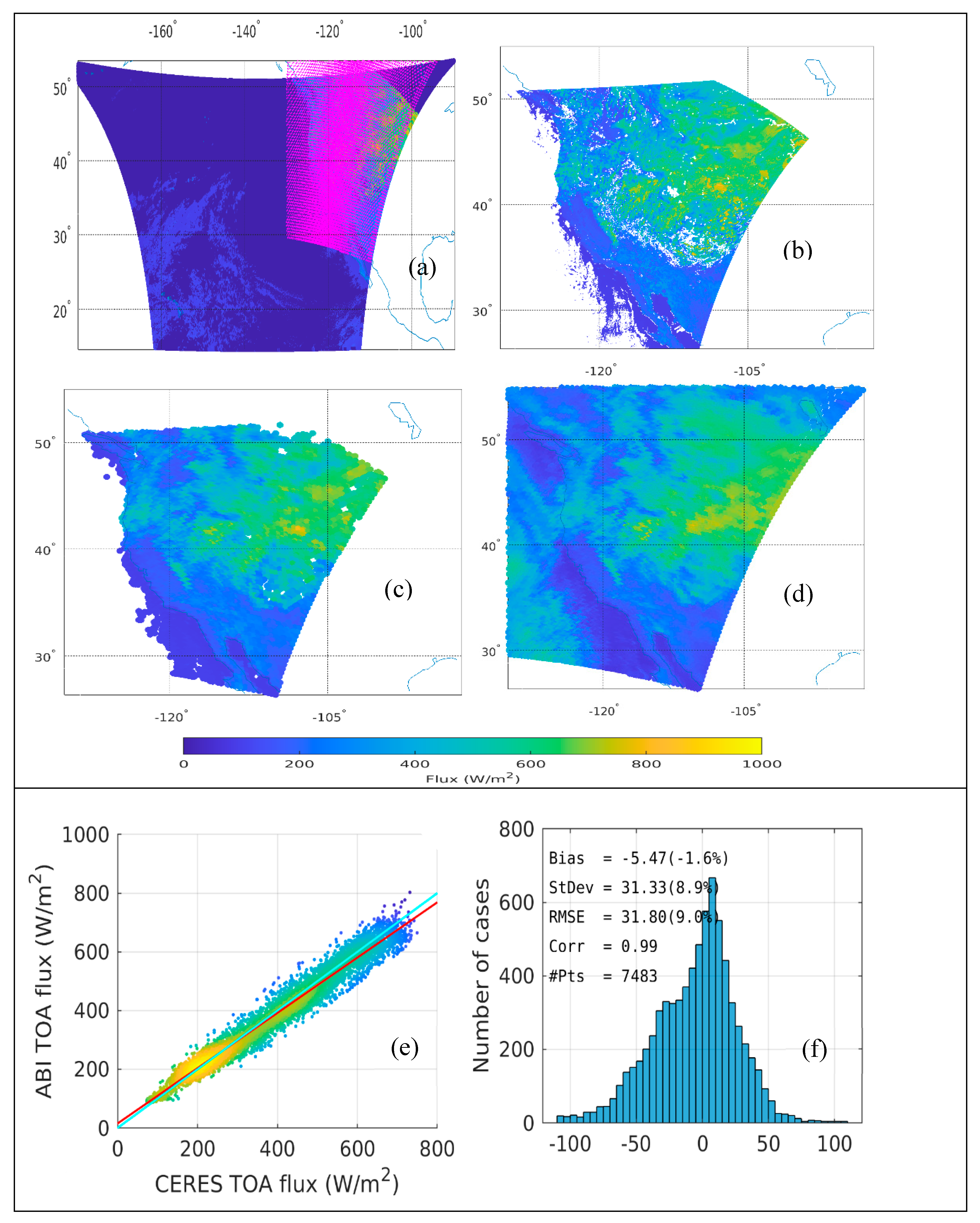
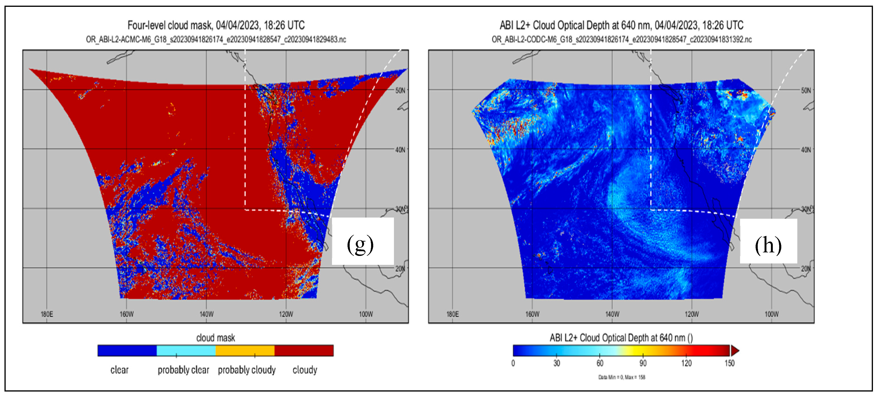

Table 1.
Wavelength, type and resolution of the six ABI bands used in this study.
| ABI Band | Central wavelength (μm) | type | Best spatial resolution |
| 1 | 0.47 | Visible | 1 |
| 2 | 0.64 | Visible | 0.5 |
| 3 | 0.86 | Near-IR | 1 |
| 4 | 1.37 | Mear-IR | 2 |
| 5 | 1.6 | Near-IR | 1 |
| 6 | 2.2 | Near-IR | 2 |
Table 2.
Number of available ABI images with pixels overlapping with CERES data within the time period from November 23 to December 1, 2022.
Table 2.
Number of available ABI images with pixels overlapping with CERES data within the time period from November 23 to December 1, 2022.
| # of overlap pixels | CERES/Terra | CERES/Aqua |
| >500 | 128 | 78 |
| >1000 | 121 | 72 |
| >5000 | 87 | 43 |
| >10000 | 47 | 21 |
| >12000 | 36 | 16 |
| >15000 | 13 | 7 |
Disclaimer/Publisher’s Note: The statements, opinions and data contained in all publications are solely those of the individual author(s) and contributor(s) and not of MDPI and/or the editor(s). MDPI and/or the editor(s) disclaim responsibility for any injury to people or property resulting from any ideas, methods, instructions or products referred to in the content. |
© 2025 by the authors. Licensee MDPI, Basel, Switzerland. This article is an open access article distributed under the terms and conditions of the Creative Commons Attribution (CC BY) license (http://creativecommons.org/licenses/by/4.0/).
Copyright: This open access article is published under a Creative Commons CC BY 4.0 license, which permit the free download, distribution, and reuse, provided that the author and preprint are cited in any reuse.


