
Submitted:
03 July 2025
Posted:
04 July 2025
You are already at the latest version
Abstract
This study presents an analysis of the impact of climate change on several factors that affect agricultural output such as soil moisture, temperature anomalies, and precipitation anomalies. The project utilizes data-powered positive deviance (DPPD) to identify farmers who are achieving better values of the aforementioned factors despite similar geographical conditions. The findings are then used to devise policies to assist other farmers in adopting similar practices. The methodology used in the study applies seasonal-trend decomposition using the loess (STL) method to analyze temporal trends of weather variables across a specific region, using data collected from various sources, such as satellite imagery and weather station readings in the state of Telangana. Similar studies done across the world demonstrate an improvement in crop yields and an increase in the resilience of farms from rapid climate change.
Keywords:
data science
; climate change
; agriculture
; data powered positive deviance
; geospatial science
1. Introduction
Climate change poses a significant challenge to global agriculture and food security. Rising temperatures, shifting precipitation patterns, and an increased frequency of extreme weather events are profoundly impacting agricultural productivity and sustainability (Vogel et al., 2019). In response to these challenges, there is an urgent need for innovative solutions that can enhance the resilience of agricultural systems to climate variability and change.
The application of data science and machine learning techniques presents a promising approach to addressing these complex issues. By leveraging large-scale datasets on weather patterns, soil moisture, and crop growth, researchers can uncover intricate relationships and patterns that inform adaptive agricultural practices and policies. This study utilizes data science methodologies to identify and promote climate-resilient agricultural practices, with a particular focus on the data-powered positive deviance (DPPD) approach.
DPPD is an emerging methodology that employs data science techniques to identify instances of positive deviance—cases where individuals or communities achieve better outcomes than their peers despite facing similar environmental constraints (Albanna & Heeks, 2018). In the context of agriculture, positive deviants are farmers who maintain higher crop yields or utilize resources more efficiently in the face of adverse climatic conditions.
The present study contributes to the growing body of research on climate-resilient agriculture by applying DPPD to analyze key factors affecting agricultural output, including soil moisture, temperature anomalies, and precipitation anomalies. By identifying positive deviances in these critical variables, we aim to uncover successful adaptation strategies that can be scaled up and replicated in other regions facing similar climatic challenges.
Our work builds upon previous studies that have demonstrated the potential of DPPD in various developmental contexts (Driesen et al., 2021; Adelhart Toorop et al., 2020). However, this research represents one of the first applications of DPPD specifically to climate resilience in agriculture at a regional scale. By focusing on the state of Telangana in India, we provide a case study of how data-driven approaches can inform localized climate adaptation strategies.
The primary objectives of this study are to:
Develop comprehensive datasets of soil moisture, temperature anomalies, and precipitation anomalies for the state of Telangana using satellite imagery and weather station data.
Apply trend analysis and DPPD methodologies to identify positive deviances in agricultural practices across the region.
Analyze the spatial and temporal patterns of these positive deviances to inform policy recommendations for promoting climate-resilient agriculture.
By achieving these objectives, this research aims to contribute to the development of evidence-based policies and programs that can enhance the adaptive capacity of agricultural systems in the face of climate change. The findings of this study have potential implications not only for Telangana but also for other regions facing similar climate-related challenges to their agricultural sectors.
2. Data
2.1. Soil Moisture
Soil moisture is a critical factor in agricultural productivity, influencing water availability for plant growth and mediating crop susceptibility to pests and diseases. Monitoring soil moisture is essential for optimizing irrigation practices and identifying areas at risk of drought or waterlogging. It serves as a direct indicator for quantifying agricultural drought.
Historically, regional-scale soil moisture measurements were sparse. However, recent advancements in land surface modeling and satellite technology have facilitated the development of comprehensive national and global soil moisture datasets. These datasets provide valuable insights into the dynamics of agricultural drought and have significantly enhanced our understanding of soil-water interactions in agricultural systems.
A key challenge in utilizing these datasets for drought quantification is establishing an accurate baseline of normal conditions. This is particularly problematic with earth observation datasets, which often have short baselines for individual instruments. Champagne et al. (2019) addressed this issue by assessing three distinct soil moisture datasets: Surface satellite soil moisture data from the Soil Moisture and Ocean Salinity (SMOS) mission (operational since 2010), A blended surface satellite soil moisture dataset from the European Space Agency Climate Change Initiative (ESA-CCI), Surface and root zone soil moisture data from the Canadian Meteorology Centre (CMC)’s Regional Deterministic Prediction System (RDPS)
Their study revealed that while short-baseline soil moisture datasets can yield consistent results compared to longer datasets, the characteristics of the baseline years are crucial. To reliably estimate the relationship between high soil moisture and high-yielding years, soil moisture baselines of 18–20 years or more are necessary.
Further research by Rossato et al. (2019) and Saha et al. (2020) underscored the significance of soil moisture in agricultural drought and emphasized the need for reliable datasets to comprehend its dynamics. These studies established a strong connection between temperature anomalies and agricultural productivity, informing our selection of datasets for this study.
Based on these findings and considering the available options (Table 1), we selected the NASA-USDA Enhanced Surface soil moisture dataset for our analysis. This dataset offers a high spatial resolution of 10 km, which is crucial for understanding localized variations in soil moisture across Telangana’s diverse landscape.
2.2. Temperature Anomalies
Temperature anomalies, defined as deviations from long-term average temperatures, play a crucial role in agricultural productivity. These variations significantly impact crop growth, development, and yield. Understanding and monitoring temperature anomalies is essential for farmers to implement effective strategies to protect crops from heat stress and optimize yields.
Extensive research has been conducted on the effects of temperature anomalies on agricultural practices and yields. Key findings include:
- Staple Crop Vulnerability: The four primary staple crops (wheat, rice, maize, and soybean) are particularly susceptible to temperature changes.
- Yield Reductions: A 1°C increase in global temperatures can dramatically affect crop production: Wheat: Approximately 6% yield decrease, Rice: 3.2% yield decrease, Maize: 7.4% yield decrease, Soybean: 3.1% yield decrease. These effects are observed in regions where temperatures are typically favorable for crop growth (Vogel et al., 2019).
-
Farmer Adaptations: In response to increasing temperature anomalies, farmers have implemented various strategies:
- On-farm techniques: Expanding cultivated land area, Adopting staggered farming approaches, such as delayed sowing of some seeds to mitigate potential crop failures.
- Off-farm practices: Diversification into livestock farming, Establishing businesses in non-agricultural sectors
However, extreme events like droughts can limit diversification opportunities, potentially forcing farmers to seek alternatives outside agriculture (Vogel et al., 2019).
Agricultural production is highly vulnerable to climate change, with temperature anomalies being the most detrimental factor affecting crop growth. The critical impact of temperature on crop yields, agricultural practices, and regional livelihoods necessitates accurate measurement and analysis of temperature anomalies to develop effective adaptive strategies (Zhao et al., 2017).
Multiple peer-reviewed surface temperature anomaly products are available (Figure 1) maintained by:
- NASA Goddard Institute for Space Studies (GISTEMP)
- National Oceanic and Atmospheric Administration (NOAA)
- National Centers for Environmental Information (NCEI) - Merged Land-Ocean Surface Temperature Analysis
- Hadley Centre/Climatic Research Unit Temperature (HadCRUT)
- Japanese Meteorological Agency (JMA)
- Berkeley Earth
While they employ different methodologies for calculating historical global and regional mean time series, they generally concur with trends and interannual variations in global annual mean values and the discrepancies can be explained with variations in data coverage and interpolation methods as well as some noise.
Most cited surface temperature analyses separate the calculation of global anomaly fields into Land Surface Air Temperature (LSAT) and Sea Surface Temperature (SST) anomaly analyses. These are then combined to create a total global surface temperature index, from which spatially averaged global and regional time series are computed. It’s important to note that this combined index is not strictly equivalent to the true surface air temperature anomaly (Cowtan et al., 2015). Uncertainty analyses for LSAT and SST are conducted separately and then combined to assess total global uncertainty.
For this research, we evaluated several datasets, considering crucial metrics such as spatial and temporal resolution. Table 2 presents the specifications of the datasets considered for our study (Lenssen et al., 2019). Based on our analysis, we selected the Copernicus ERA5-Land monthly averaged data from 1950 to present to create in-situ datasets for temperature anomalies. This choice was driven by the need for long-term data with sufficient spatial resolution for our analysis of Telangana’s agricultural regions.
2.3. Precipitation Anomalies
Precipitation anomalies, defined as deviations from long-term average rainfall patterns, pose significant challenges to agricultural systems worldwide, with disproportionate effects on developing nations. Countries with high dependence on agricultural employment, rapid population growth, and elevated levels of water stress are particularly vulnerable to rainfall variability (Zaveri et al., 2018; Palagi et al., 2020; Felton et al., 2019). Since the mid-20th century, anthropogenic climate forcing has doubled the probability of concurrent warm and dry years in the same location, with tropics and subtropics facing an increased frequency of record-breaking dry events (Zaveri et al., 2018).
While the effects of rainfall variability on crop yields and productivity have been widely studied, the consequences of changes in cropland areas and associated deforestation are less understood and yet to be quantified on a global, disaggregated scale. Research has shown that repeated dry anomalies lead to cropland expansion, particularly in developing countries dominated by smallholder farming, likely as a compensation for lower yields during dry periods. This finding is corroborated by observations of forest cover reductions in areas of cropland expansion due to dry anomalies, and the halting of cropland expansion in regions where infrastructure buffers yield from rainfall anomalies (Zaveri et al., 2018).
The socioeconomic implications of precipitation anomalies are significant. Rainfall anomalies exacerbate income inequality in agriculture-dependent economies, with climate projections suggesting worsening disparities over time. While climate change is likely to increase income inequality between countries, its differential impacts across income classes within countries remain less understood. These findings underscore the urgent need for inclusive and sustainable development policies, especially in highly exposed countries, to mitigate negative impacts on lower-income populations and the environment (Palagi et al., 2020).
For our analysis of precipitation anomalies in Telangana, we evaluated several gridded precipitation anomaly datasets. However, due to limitations in spatial accuracy and temporal availability, we opted to create in-situ datasets using Copernicus ERA5 data. This decision was driven by the need for high-resolution, locally relevant data to accurately assess the impact of precipitation anomalies on agricultural resilience in the region. By focusing on these locally derived precipitation anomaly datasets, our study aims to provide a nuanced understanding of rainfall variability in Telangana and its implications for agricultural practices and policies. This approach allows for a more targeted analysis of climate resilience strategies in the context of local agricultural systems and socioeconomic conditions, addressing the research gaps in quantifying global impacts, assessing comprehensive effects, and exploring adaptive strategies for smallholder farmers
in vulnerable regions.

Table 3.
Precipitation Anomaly Datasets .
| Dataset | Spatial Resolution | Temporal resolution | Frequency |
| NOAA NCEP CPC CAMS_OPI v0208 | 2.5°x2.5° | 1979 - Present | Monthly |
| Climate Hazards Group InfraRed Precipitation with Station data |
0.05°x0.0 5° |
1981 - 2022 | Daily, monthly |
More datasets available at: https://psl.noaa.gov/data/gridded/tables/precipitation.html
3. Methodology
3.1. Methodology for Anomaly Calculation
The methodology employed in this study for calculating both temperature and precipitation anomalies aims to elucidate temporal variations in climate patterns. Anomalies are determined by subtracting a long-term mean from the available data for a given period, thus isolating and identifying deviations from the mean. This approach facilitates the identification of trends, patterns, and changes, providing valuable insights into the characteristics and behavior of both temperature and precipitation.
Our method draws inspiration from established practices in climate science. For instance, NASA Climate utilizes a 30-year reference period (1951-1980) to calculate temperature anomalies at given weather stations. Similarly, the Japan Meteorological Association employs a 1991-2020 baseline for estimating global mean temperature anomalies, using a 5° x 5° grid box system worldwide and weighting anomalies by the land-to-ocean ratio and area of each grid box. This methodology is equally applicable to precipitation data.
The anomaly calculation process for both temperature and precipitation comprises three primary steps:
- Data acquisition and baseline establishment: Global temperature and precipitation data are obtained, and climatological averages are calculated over a 30–50-year period using statistical methods such as the arithmetic mean or the climatological mean. The choice of the baseline period is critical, as it can significantly influence the results and the interpretation of the anomalies for both variables.
-
Anomaly computation: Deviations of specific months or years from the average values are determined for both temperature and precipitation. The anomaly is calculated using the formula:This formula is applied consistently to both temperature and precipitation data.
- Spatial analysis and visualization: The calculated anomalies for both temperature and precipitation are used to create maps displaying variations at different geographical levels. GIS software is utilized to overlay the anomaly data on geographical boundaries such as districts or mandals, providing a visual representation of regions experiencing abnormal conditions in terms of both temperature and precipitation.
This methodology, illustrated in Figure 2, allows for comprehensive monitoring of climate change impacts across different regions and facilitates the identification of areas experiencing significant deviations from long-term averages in both temperature and precipitation patterns. By applying this consistent approach to both variables, we can analyze potential correlations and combined effects of temperature and precipitation anomalies on agricultural systems.
3.2. Methodology for DPPD Calculation
The Data-Powered Positive Deviance (DPPD) methodology is a powerful approach to identifying and understanding exceptional performance in the context of environmental and agricultural data. By leveraging time series data and advanced statistical techniques, DPPD helps uncover locations that demonstrate positive trends despite adverse conditions. These positive deviants can offer valuable insights into effective practices and strategies that can be adopted more broadly to enhance resilience and productivity. This methodology involves a comprehensive process that includes data preparation, time series decomposition using Seasonal and Trend decomposition using Loess (STL), trend extraction, linear regression, spatial iteration, and the identification and mapping of positive deviants.
The STL method decomposes the time series into three distinct components:
Where:
is the trend component, representing the underlying direction or pattern in the data over time.
is the seasonal component, capturing regular fluctuations due to seasonal effects.
is the residual component, encompassing random noise not explained by the trend or seasonal components.
To estimate these components, the STL algorithm uses iterative Loess smoothing. Loess (locally estimated scatterplot smoothing) is a non-parametric method that fits multiple regressions in localized subsets of the data to produce a smooth curve. The regression function for Loess smoothing is defined as:
Where are weights calculated based on the distance of from, giving more influence to points closer to
After decomposing the time series, we isolate the trend component for further analysis. The trend component is essential as it reveals the long-term progression in the data, which is critical for identifying positive deviants. A linear regression is performed on against time t to quantify the trend:
Where:
is the y-intercept, representing the value of the trend component at the start of the time.
is the slope, indicating the rate of change in the trend component over time.
is the error term, capturing deviations of the observed trend from the fitted line.
The slope is calculated using the least squares method, which minimizes the sum of the squares of the residuals.
The decomposition and regression steps are repeated for each location in the area of interest. This iterative process ensures that we obtain a slope for each location, capturing the localized trend dynamics.
The trend scores from all locations are compiled into an array Where n is the number of locations. This array represents the spatial distribution of trend strengths across the study area. Positive deviants are identified by comparing each with each other or by filtering for a percentile value.
Finally, the trend scores and positive deviance indicators are mapped to their geographic coordinates for spatial analysis. This spatial visualization helps identify geographical patterns and clusters of positive deviants, providing insights into regions exhibiting exceptional performance. This methodology offers a framework for identifying and analyzing positive deviance in environmental and agricultural contexts. By systematically decomposing time series data and performing detailed statistical analyses, this approach highlights areas of exceptional performance that can provide valuable insights into sustainable practices and adaptive strategies. The identification and study of these positive deviants enables researchers and practitioners to uncover underlying factors contributing to success, fostering knowledge transfer and innovation.
4. Results & Discussion
In this study, we created a dataset of soil moisture, temperature anomalies, and precipitation anomalies for the state of Telangana, collected from various sources including satellite imagery and weather station readings. Our trend analysis aimed to identify positive deviances in these environmental parameters, where positive deviances were defined as instances where farmers achieved better crop yields or used less water despite facing similar environmental conditions as their peers.
All the values in the analysis have been scaled -1 to 1 to make comparisons easier to conduct between each district. For soil moisture deviances, the analysis revealed significant regional variations. The regions with the highest positive soil moisture deviance included Chinnambavi, Pentlavelli, Kuravi, Adavidevulapally, and Dornakal, with normalized deviance values of 1, 0.969, 0.553, 0.533, and 0.529 respectively. Conversely, the regions with the lowest soil moisture deviance were Balapur, Shamshabad, Rajendranagar, Hayathnagar, and Bandlaguda, with normalized deviance values of -1, -0.965, -0.923, -0.890, and -0.886 respectively (see Figure 3 and Table 4 and Table 5).
Temperature anomalies also showed distinct patterns of positive deviance. The regions with the highest positive temperature anomalies deviance were Aswaraopeta, Dammapeta, Sathupally, Mulakalapally, and Annapureddipalle, with normalized deviance values of -1, -0.976, -0.958, -0.883, and -0.877 respectively. On the other hand, regions with the lowest temperature anomalies deviance included Naspur, Bheemaram, and Mandamarri, each with normalized deviance values around 1 (see Figure 4 and Table 6 and Table 7).
Precipitation anomalies also exhibited notable regional variations. The top regions with positive precipitation anomalies deviance were Dhoolumitta, Masaipet, Chowtakur, Chandur, and Mosra, with normalized deviance values of -1, -0.997, -0.993, -0.990, and -0.986 respectively. In contrast, the regions with the lowest precipitation anomalies deviance were Abdullapurmet, Achampet, Adavidevulapally, Addagudur, and Addakal, with normalized deviance values of 1, 0.997, 0.993, 0.990, and 0.986 respectively (see Figure 5 and Table 8 and Table 9).
The findings indicate that regions like Chinnambavi and Pentlavelli exhibit remarkable positive deviances in soil moisture, suggesting effective water use and soil management practices that could be modeled in other areas. Similarly, regions such as Aswaraopeta and Dammapeta show significant positive deviances in temperature anomalies, indicating possible resilience strategies to temperature variations. Furthermore, regions like Dhoolumitta and Masaipet, with high positive deviances in precipitation anomalies, highlight successful adaptation to rainfall variability.
These results are made accessible through the DiCRA platform, which can be explored at DiCRA GitHub and DiCRA UNDP. This platform allows users to delve into the data and identify positive deviances in their own regions. By collaborating with government officials, we have also provided training and support to farmers, helping them implement these best practices on their farms. This study offers crucial insights for aiding farmers in adapting to climate change and provides a valuable resource for policymakers, researchers, and other stakeholders. The data and platform also help understand the overall patterns of soil moisture and precipitation in the region, identifying areas more susceptible to drought, thus aiding in the development of targeted interventions to promote resilience and sustainability.
5. Conclusions
In this work, we applied a Data-Powered Positive Deviance framework to analyze high-resolution geospatial time series data of soil moisture, temperature anomalies, and precipitation anomalies in Telangana, India. This allowed us to identify farming sites consistently outperforming their peers under similar climatic conditions. By integrating satellite data (NASA-USDA Enhanced Surface soil moisture) and reanalysis products (Copernicus ERA5-Land), performing seasonal-trend decomposition (STL), and estimating linear trends, we identified “positive deviants” whose resilience indicates potential yield advantages. Although constrained by the relatively short temporal coverage (2015–2020) of soil moisture data, inherent uncertainties in reanalysis products, and computational limitations, our analysis demonstrates the practicality and utility of deploying the DiCRA platform to deliver targeted, data-driven insights to policymakers and farming communities.
Looking ahead, integrating these anomaly-based deviance signals with ground-truth crop-yield records would enable quantitative validation of resilience gains. Expanding the framework to additional drought-prone regions will test broader applicability, while publicly releasing our preprocessing and GIS workflows will enhance reproducibility, transparency, and community adoption. To conclude, the approach provides a scalable foundation for informing climate-resilient agricultural practices through open, data-driven decision support.
References
- Albanna, B., & Heeks, R. (2018). Positive deviance, big data, and development: A systematic literature review. The Electronic Journal of Information Systems in Developing Countries, 85(1), e12063. [CrossRef]
- Adelhart Toorop, R., Krupnik, T. J., Roy, D., Kumar, V., & Ghosh, A. (2020). Using a positive deviance approach to inform farming systems redesign: A case study from Bihar, India. Agricultural Systems, 185, 102942. [CrossRef]
- Driesen, J., Reisch, L., & Lucius-Hoene, G. (2021). Data-powered positive deviance during the SARS-CoV-2 pandemic—An ecological pilot study of German districts. International Journal of Environmental Research and Public Health, 18(18), 9765. [CrossRef]
- Copernicus Climate Data Store. (n.d.). Soil moisture gridded data from 1978 to present. [CrossRef]
- Bolten, J. D., Zhan, X., & Crow, W. T. (2010). Evaluating the utility of remotely sensed soil moisture retrievals for operational agricultural drought monitoring. IEEE Transactions on Geoscience and Remote Sensing, 3(1), 57–66. [CrossRef]
- Bolten, J. D., & Crow, W. T. (2012). Improved prediction of quasi-global vegetation conditions using remotely sensed surface soil moisture. Geophysical Research Letters, 39. [CrossRef]
- Mladenova, I. E., Bolten, J. D., & Anderson, M. C. (2017). Intercomparison of soil moisture, evaporative stress, and vegetation indices for estimating corn and soybean yields over the U.S. IEEE Journal of Selected Topics in Applied Earth Observations and Remote Sensing, 10(4), 1328–1343. [CrossRef]
- Sazib, N., Mladenova, I. E., & Bolten, J. D. (2018). Leveraging the Google Earth Engine for drought assessment using global soil moisture data. Remote Sensing, 10(8), 1265. [CrossRef]
- Entekhabi, D., et al. (2010). The soil moisture active passive (SMAP) mission. Proceedings of the IEEE, 98(5), 704–716. [CrossRef]
- O’Neill, P. E., et al. (2016). SMAP L3 radiometer global daily 36 km EASE-grid soil moisture, version 4. NASA National Snow and Ice Data Center. [CrossRef]
- Sazib, N., Bolten, J. D., & Mladenova, I. E. (2022). Leveraging NASA Soil Moisture Active Passive for assessing fire susceptibility and potential impacts over Australia and California. IEEE Journal of Selected Topics in Applied Earth Observations and Remote Sensing, 15, 779–787. [CrossRef]
- Rossato, L., Assad, E. D., & Pires, G. F. (2017). Impact of soil moisture on crop yields over Brazilian semiarid. Frontiers in Environmental Science, 5, 73. [CrossRef]
- Saha, A., Panigrahy, S., & Kundu, N. (2019). Assessment and impact of soil moisture index in agricultural drought estimation using remote sensing and GIS techniques. Proceedings 2019, 7, 2. [CrossRef]
- Champagne, B., McNairn, H., & Berg, A. (2019). Impact of soil moisture data characteristics on the sensitivity to crop yields under drought and excess moisture conditions. Remote Sensing, 11, 372. [CrossRef]
- Japan Meteorological Agency. (n.d.). Global surface temperature anomalies (seasonal). Retrieved from https://web.archive.org/web/20220623113538/https:/ds.data.jma.go.jp/tcc/tcc/products/gwp/temp/explanation.html.
- Vogel, E., Donat, M. G., Alexander, L. V., & Karoly, D. J. (2019). The effects of climate extremes on global agricultural yields. Environmental Research Letters, 14. [CrossRef]
- Zhao, C., Liu, B., Piao, S., et al. (2017). Temperature increase reduces global yields of major crops in four independent estimates. Proceedings of the National Academy of Sciences, 114(35), 9326–9331. [CrossRef]
- Lenssen, N. J. L., Schmidt, G. A., & Hansen, J. E. (2019). Improvements in the GISTEMP uncertainty model. Journal of Geophysical Research: Atmospheres, 124, 6307–6326. [CrossRef]
- NOAA PSL. (n.d.). CPC Global Unified Temperature data. Retrieved from https://psl.noaa.gov.
- Fick, S. E., & Hijmans, R. J. (2017). WorldClim 2: New 1 km spatial resolution climate surfaces for global land areas. International Journal of Climatology, 37(12), 4302–4315. [CrossRef]
- University of East Anglia Climatic Research Unit, Harris, I. C., & Jones, P. D. (2019). CRU TS4.06: Climatic Research Unit (CRU) Time-Series (TS) version 4.06 of high-resolution gridded data of month-by-month variation in climate (Jan. 1901–Dec. 2018). Centre for Environmental Data Analysis.
- Karger, D. N., Conrad, O., Böhner, J., et al. (2017). Climatologies at high resolution for the Earth’s land surface areas. Scientific Data, 4, 170122. [CrossRef]
- Dunn, R. J. H., Morice, C. P., Willett, K. M., et al. (2020). Development of an updated global land in situ-based data set of temperature and precipitation extremes: HadEX3. Journal of Geophysical Research: Atmospheres, 125, e2019JD032263. [CrossRef]
- Rohde, R. A., & Hausfather, Z. (2020). The Berkeley Earth land/ocean temperature record. Earth System Science Data, 12, 3469–3479. [CrossRef]
- Muñoz Sabater, J. (2021). ERA5-Land monthly averaged data from 1950 to 1980. Copernicus Climate Change Service (C3S). [CrossRef]
- Zaveri, E., et al. (2020). Rainfall anomalies are a significant driver of cropland expansion. Proceedings of the National Academy of Sciences, 117(19), 10225–10233. [CrossRef]
- Palagi, E., et al. (2022). Climate change and the nonlinear impact of precipitation anomalies on income inequality. Proceedings of the National Academy of Sciences, 119, e2203595119. [CrossRef]
Figure 1.
Temperature anomalies from diff. sources: NASA, NOAA, Hadley, JMA, Berkeley Earth, Cowtan.
Figure 1.
Temperature anomalies from diff. sources: NASA, NOAA, Hadley, JMA, Berkeley Earth, Cowtan.
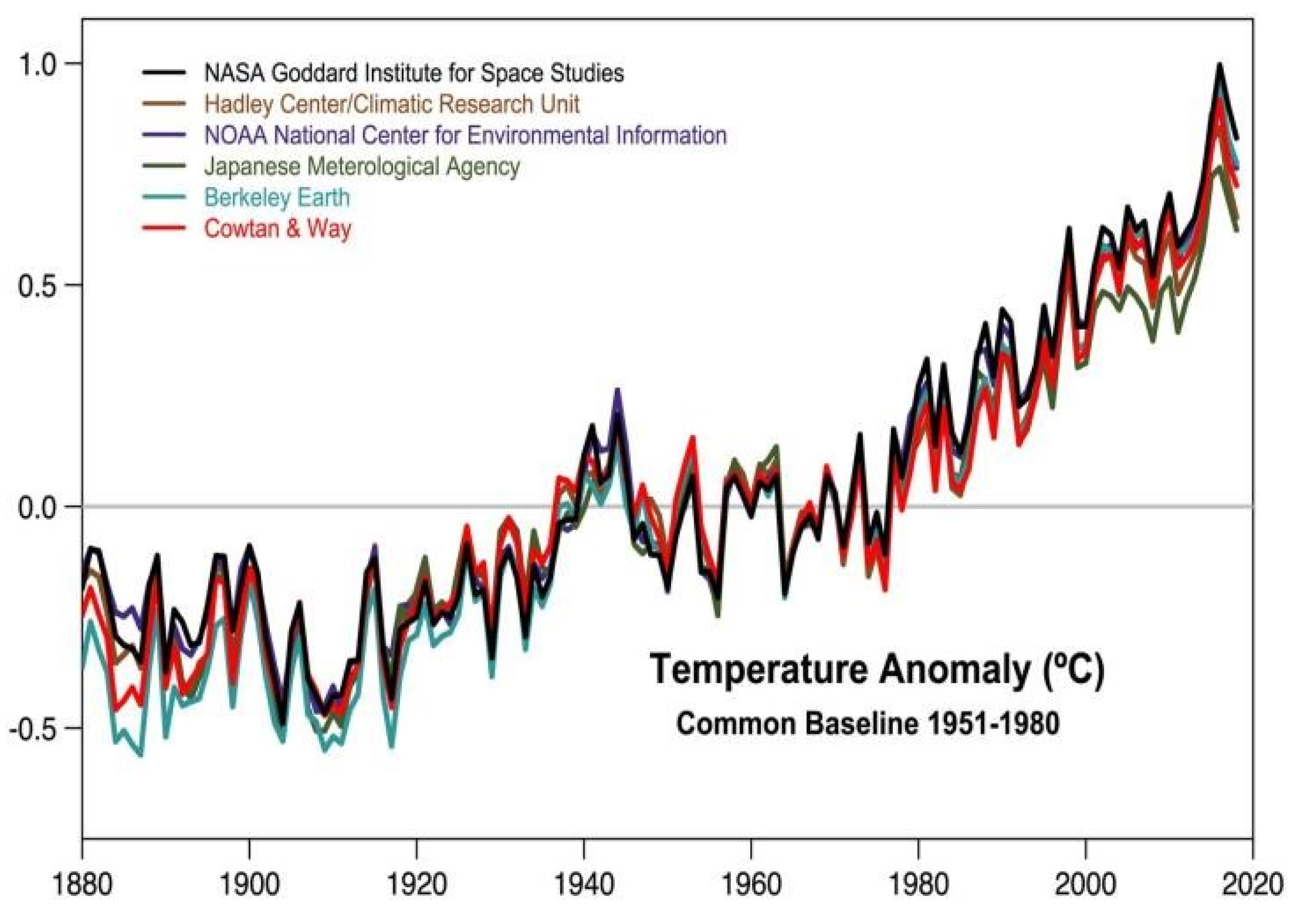
Figure 2.
Workflow of methodology to calculate temperature anomalies.
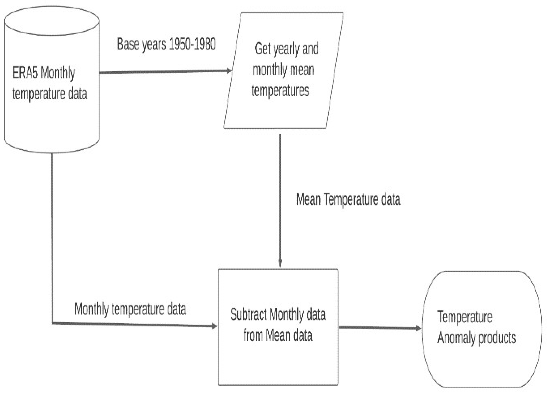
Figure 3.
Telangana Mandal deviances in soil moisture.
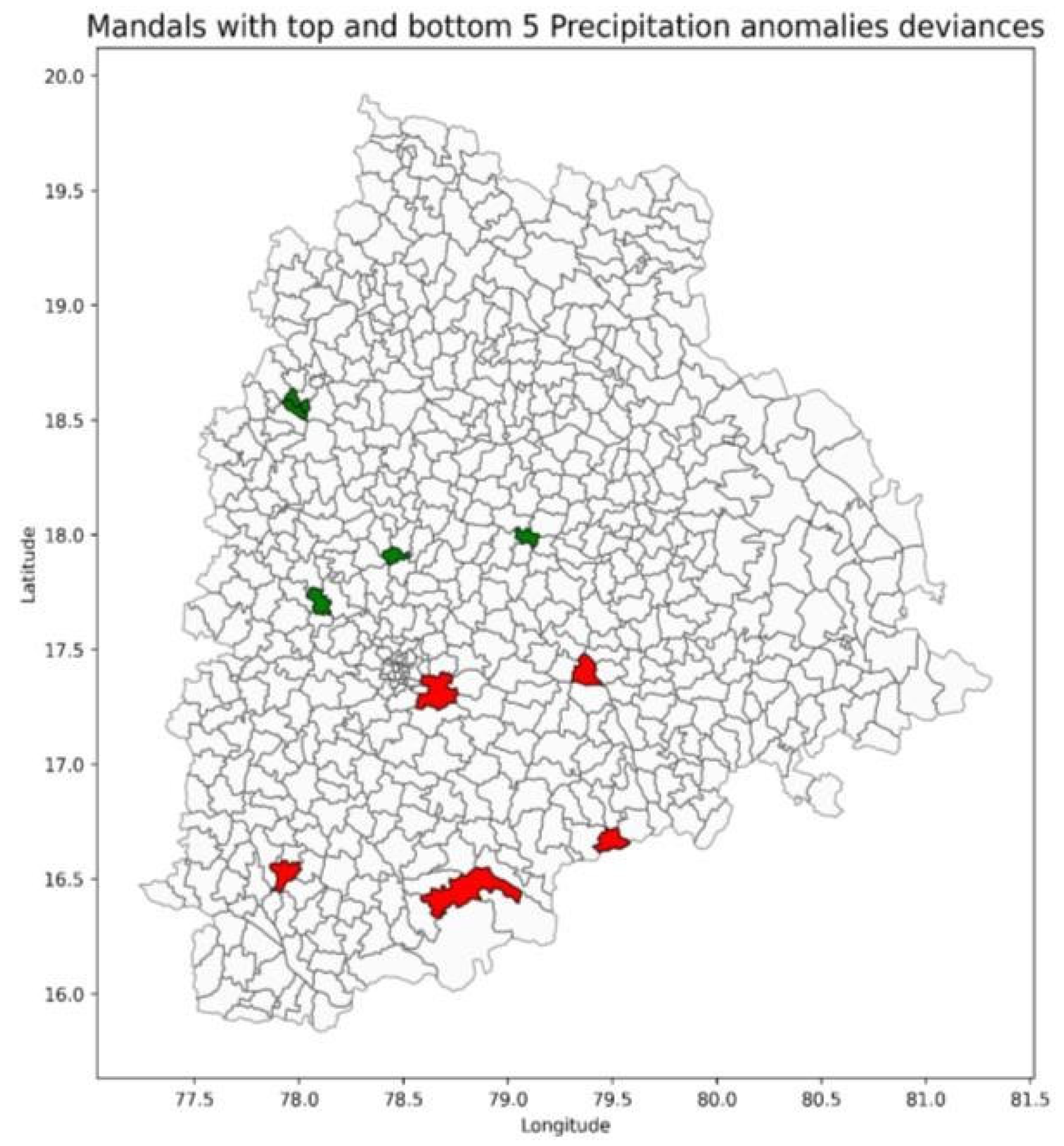
Figure 4.
Telangana Mandal deviances in Temperature anomalies.
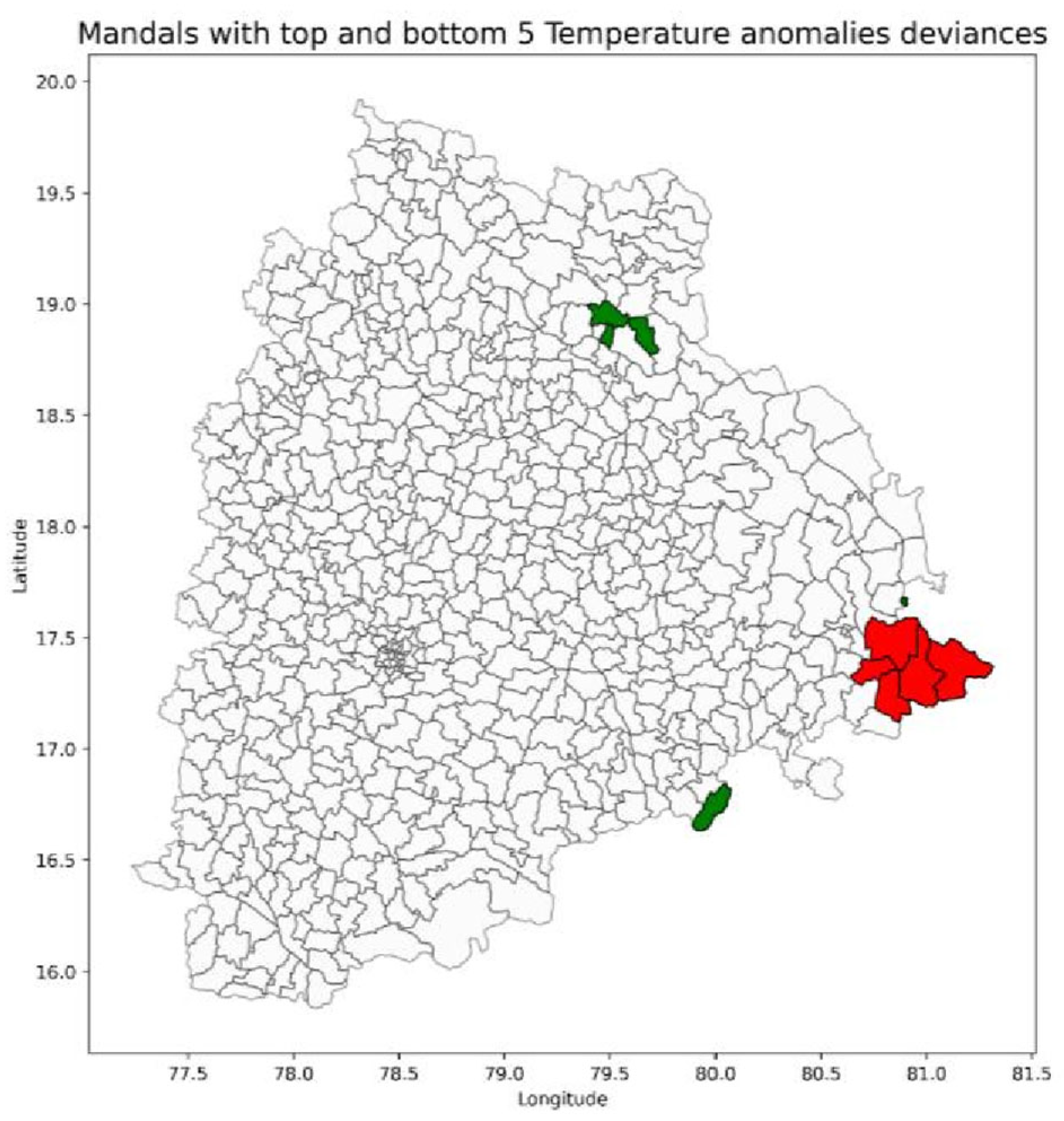
Figure 5.
Telangana Mandal deviances in precipitation anomalies.
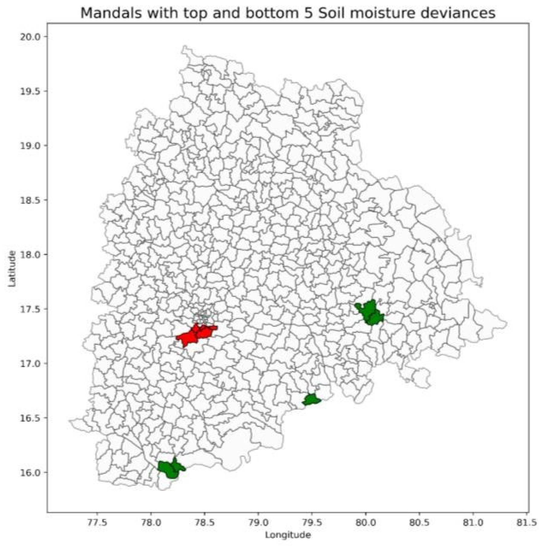
Table 1.
Soil Moisture Datasets.
| Name of dataset |
Spatial Resolution |
Temporal Resolution | Frequency |
| Copernicus Climate Change Service Soil moisture (Copernicus) | 0.25°x0.25° | 1978 to present |
10 days |
| NASA - USDA Global Surface soil moisture (Bolten et. al, 2010) |
0.25°x0.25° | 2015-2020 | 3 days |
| NASA - USDA Enhanced Surface soil moisture (Bolten et. al, 2010) | 10-km | 2015-2020 | 3 days |
Table 2.
Temperature Anomaly Datasets.
| Name of dataset | Spatial Resolution | Temporal Resolution | Frequency |
| CPC | 0.5°x0.5° | 1979 - present | daily |
| WorldClim 2.1 (Fick et. al, 2017) |
2.5 arc minute | 1970 - 2018 | monthly |
| CRU TS v4.06 (Harris et.al.,2022) | 0.5°x0.5° | 1901 - 2021 | monthly |
| CHELSA v2.1 (Karger et.al, 2017) | 30 arc second | 1980 - 2019 | monthly |
| HADEx3 (Dunn et.al, 2020) | 1.25° x 1.875° | 1901 - 2018 | daily |
| Berkeley Earth (Rohde et. al, 2021) | 1°x1° | 1833 - Present | monthly |
Table 4.
Region With Positive Soil Moisture deviance (TOP 5):.
| Mandal Name | Normalized deviance value |
| Adavidevulapally | 0.533208 |
| Chinnambavi | 1 |
| Dornakal | 0.529491 |
| Kuravi | 0.552656 |
| Pentlavelli | 0.968607 |
Table 5.
Region With Positive Soil Moisture deviance (BOTTOM 5):.
| Mandal Name | Normalized deviance value |
| Balapur | -1 |
| Shamshabad | -0.96492 |
| Rajendranagar | -0.92257 |
| Hayathnagar | -0.88956 |
| Bandlaguda | -0.88618 |
Table 6.
Region With Positive Temperature Anomaly deviance (TOP 5):.
| Mandal Name | Normalized deviance value |
| Aswaraopeta | -1 |
| Dammapeta | -0.97605 |
| Sathupally | -0.95808 |
| Mulakalapally | -0.88323 |
| Annapureddipalle | -0.87725 |
Table 7.
Region With Positive Temperature Anomaly deviance (BOTTOM 5): .
| Mandal Name | Normalized deviance value |
| Naspur | 0.997006 |
| Bheemaram | 1 |
| Mandamarri | 1 |
Table 8.
Region With Positive Precipitation Anomaly deviance (TOP 5): .
| Mandal Name | Normalized deviance value |
| Dhoolumitta | -1 |
| Masaipet | -0.99657 |
| Chowtakur | -0.99313 |
| Chandur | -0.9897 |
| Mosra | -0.98626 |
Table 9.
Region With Positive Precipitation Anomaly deviance (BOTTOM 5): .
| Mandal Name | Normalized deviance value |
| Abdullapurmet | 1 |
| Achampet | 0.996643 |
| Adavidevulapally | 0.993208 |
| Addagudur | 0.989825 |
| Addakal | 0.986468 |
Disclaimer/Publisher’s Note: The statements, opinions and data contained in all publications are solely those of the individual author(s) and contributor(s) and not of MDPI and/or the editor(s). MDPI and/or the editor(s) disclaim responsibility for any injury to people or property resulting from any ideas, methods, instructions or products referred to in the content. |
© 2025 by the authors. Licensee MDPI, Basel, Switzerland. This article is an open access article distributed under the terms and conditions of the Creative Commons Attribution (CC BY) license (http://creativecommons.org/licenses/by/4.0/).
Copyright: This open access article is published under a Creative Commons CC BY 4.0 license, which permit the free download, distribution, and reuse, provided that the author and preprint are cited in any reuse.


