Sparse Data-Driven Model for Monitoring of Industrial Process Based on Distributed Feature Extraction Neural Network

Zhen Li; Yibin Han; Yanxia Yang

doi:10.20944/preprints202507.0364.v1

Submitted:

02 July 2025

Posted:

04 July 2025

You are already at the latest version

Abstract

Modern industrial processes store a large amount of process data in the integration of subsystems or subprocesses, which creates conditions for data-driven models. However, due to a few features in various tasks possessing a direct correlation, there are many variables and complex relationships, which may result in incomplete input information. To address this problem, this paper proposes a task decomposition and feature integration-based distributed process monitoring model. Firstly, a sparse subspace clustering algorithm is introduced for task decomposition. This algorithm divides the original space into several interactive feature subspaces and allocates weights to quantify the contribution of the subtask simultaneously. Secondly, based on the divided features, a distributed framework for spatial feature integration is proposed. The framework constructs a differentiated parallel coding network by designing a structural self-organization mechanism, which achieves feature extraction and fusion of each subspace. Finally, a collaborative optimization algorithm is proposed to optimize the network parameters of each sub-model at the same time to ensure the accuracy of the model. To demonstrate the effectiveness of this data modeling method, we tested it in several benchmark data sets and a high-dimensional nonlinear system. The experimental results show that the model has better performance in data dimensionality reduction.

Keywords:

process monitoring model

;

sparse feature

;

sparse subspace clustering

;

collaborative optimization algorithm

;

distributed neural network

Subject:

Computer Science and Mathematics - Artificial Intelligence and Machine Learning

I. INTRODUCTION

In the past decades, process monitoring model (PMM) has been widely used for variables monitoring, fault diagnosis, and performance evaluation in industrial processes [1,2,3]. With the development of acquisition equipment, automation, and transmission technology, a mass of irrelevant process variables are stored, industrial process monitoring model is confronted with the problem of feature sparsity [4,5,6]. The inflow of large-scale incomplete information will increase the model deviation and the difficulty of parameter training [7,8,9]. Therefore, it is urgent to develop a multitask clustering (MTC) algorithm that 1) not only automatically mines the potential relationship of variables from the data 2) but also reduces the size of the problem and improves the efficiency of model processing. To achieve the above goal on MTC, we need to resort to two research areas—multitask clustering and model design.

To divide the feature space, many clustering algorithms have been proposed. Meanwhile, partitioning methods such as k-means are probably one of the most frequently used techniques. As widely reported in the literature, however, the performance of this kind of algorithm is unstable due to the influence of the initially selected central sample [10,11,12]. To improve the algorithm performance, there have been many research proposals [13,14]. In [13], Modha et al. proposed a feature weighted k-means clustering algorithm, to be the one that yields the clustering that simultaneously minimizes the average within-cluster dispersion and maximizes the average between-cluster dispersion along all the feature spaces. In [14], Luo et al. proposed a spatial constrained k-means clustering algorithm, which adopted the spatial constraints into the hierarchical K-means clusters on each image level. This kind of algorithm can only get a single spherical partition of the data input space. To further mine data information, some more complex clustering methods are proposed [15,16]. For example, Louhichi et al. proposed a density-based algorithm for discovering clusters to obtain the local density change in a large database with noise [15]. Cheng et al. proposed a multistage random sampling clustering algorithm based on fuzzy c-means, which effectively improves computational efficiency by significantly reducing the clustering time [16]. However, all of the proposed algorithms in [13,14,15,16] are aimed at linear separable data space, and it is hard to find suitable clustering contours and stable clustering results for indivisible data. By introducing a kernel function, the algorithm based on the kernel function can project the linearly inseparable data in the input space into the high-dimensional space to make it separable [17,18]. In [17], Chiang et al. extended the support vector clustering to an adaptive cell growing model that maps data points to a high-dimensional feature space through a desired kernel function. In [18], Fan et al. designed a self-adaptive kernel k-means algorithm, which can adjust the kernel parameter automatically according to the data structure. The above clustering methods all contain division criteria based on distance measurement. With the increase of data dimensions, the data are almost equidistant, and the distance metric becomes meaningless. Manifold Learning considers that high-dimensional data will exhibit dense aggregation in a low-dimensional space. Therefore, the subspace clustering method (SCM) is derived to find the low-dimensional subspace in high-dimensional data [19,20]. For example, Kang et al. proposed a unified multi-view subspace clustering model that incorporates the graph learning from each view, the generation of basic partitions, and the fusion of consensus partitions [19]. Xu et al. adopt soft subspace clustering to solve the problem of rule redundancy of fuzzy systems in high-dimensional data [20]. Several articles have mentioned that SCM provides a variety of perspectives for feature extraction of sparse data to ensure the maximum use of input information [20,21,22,23].

After the feature space is divided, the original problem becomes a multi-tasking problem. There are many models based on local-global ideas that can be used to solve the above problem [24,25,26]. For example, Koker et al. proposed a parallel feed-forward neural network structure is used in the prediction of Parkinson’s Disease [24]. Gupta et al. proposed a new technique to train deep neural networks over several data sources, which allowed for deep neural networks to be trained using data from multiple entities in a distributed fashion [25]. Cao et al. proposed a fuzzy rough neural network via distributed parallelism, where each model is transformed into a multi-objective optimization problem [26]. The subnets of these models are often isomorphic and are only suitable for cases where the feature subset is similar [27,28,29,30]. MNN adopts the divide-and-conquer strategy, divides the main tasks into several simple subtasks, and obtains heterogeneous subnet modules according to different tasks, thus improving the overall generalization performance [31,32]. In [31], Li et al.（引言里的et al.是不是都要斜体啊？） introduced an enhanced feature-weighted modular neural network (MNN), in which each RBF subnetwork was independently constructed, and the final output is obtained by aggregating the outputs of all subnetworks through a weighted summation, where the weights reflected the contribution of each subnetwork. In [32], Valdez et al. proposed a new hybrid approach combining particle swarm optimization and genetic algorithms, which used fuzzy logic to integrate the results of subnetwork modules in MNN for face recognition. In the follow-up research, a series of methods have been proposed that MNN can independently generate heterogeneous subnetworks to solve online problems [33,34]. For example, Qiao et al. proposed an online self-adaptive MNN for time-varying systems, which adopted a single-pass subtractive cluster algorithm to divide the input space and used a fuzzy strategy to integrate the results of subnetworks [33]. Loo et al. proposed a novel self-regulating algorithm to generate an optimum growing multi-experts network structure, which adopted a modified fully self-organized simplified adaptive resonance theory and self-adaptive learning rates for gradient descent learning rules to dynamically grow and prune the MNN’s structure at a fixed step [34]. However, MNN has the problem of long learning time due to the slow convergence rate of gradient decline [35,36,37,38]. Moreover, the preset output weight makes it difficult to obtain an accurate prediction output according to the change of input distribution [39].

In this paper, to fully exploit sparse data information and obtain stable modeling performance, a task decomposition and feature integration-based distributed process monitoring model is proposed to realize the feature fusion of multi-task subspace. Our proposed PMM has the following properties: Firstly, an improved sparse subspace clustering algorithm (ISSC) constructs the affinity matrix by the distance between the sample and the subspace to obtain dense low-rank subspaces. This ISSC algorithm can retain the correlation information of features while efficiently feature division is achieved. Secondly, a distributed framework for spatial feature integration constructs differentiated coding networks in parallel, and designs model evaluation indexes according to subspace sparsity of each coding network, which can achieve feature extraction and integration of each subspace. Thirdly, a collaborative optimization algorithm optimizes the network parameters of each sub-model at the same time to ensure the accuracy of the model, which can maintain the accuracy of PMM.

The rest of this paper is organized as follows. Section II briefly reviews and discusses the basics of SSC. Section III details the proposed PMM framework, including ISSC and the distributed neural network. Then, the parameter update process of the distributed neural network is given in Section IV. Section V reports some experimental results of the proposed PMM, which demonstrate some merits in learning speed and modeling accuracy against other existing methods. Section VI concludes this paper with some remarks.

II. Problem Formulation and Preliminaries

Industrial processes have accumulated a large number of process variables, most of which have no significant correlation. Sparse coding advocates building a more concise feature representation [40,41]. The data set is divided into meaningful blocks to highlight the local information, so that these blocks are not related to each other to the maximum extent, so as to obtain dense feature representation.

Given a feature x and a basis pool U =[u₁, u₂, ..., u_k ], sparse coding aims at sparsely and linearly reconstructing the feature to be encoded, x=v₁u₁+v₂u₂+···+v_ku_k. Here, sparseness means only a small fraction of elements in v are non-zero. The optimization problem of sparse coding can be calculated as follows

\min_{v} {‖v‖}_{0} \begin{matrix} s t . \begin{matrix} x = U v \end{matrix} \end{matrix},

(1)

where, ║v║₀ means the number of non-zero elements in v. However, the minimization of l₀ norm is an NP hard problem. In many practical applications, reconstruction error is inevitable and often difficult to estimate in advance. Therefore, it is beneficial to jointly optimize both the sparsity of the coefficients and the reconstruction error. Accordingly, the objective function of sparse coding can be reformulated as follows

\min_{U, v} {‖x - U v‖}^{2} \begin{matrix} + λ {‖v‖}_{1} & s t . \begin{matrix} u_{m} \leq 1 \end{matrix} \end{matrix},

(2)

where, the first term of Eq. (2) is the reconstruction error, and the second term is used to control the sparsity of the sparse codes v. And λ is the tradeoff parameter used to balance the sparsity and the reconstruction error.

III. Architecture of ISSC-DFNN

Under a global-local framework, ISSC-DFNN is composed of four primary components: the input layer, Subspace partition, feature extraction, and feature integration, as illustrated in Figure 1. The structure and functionality of each layer are detailed as follows

Input: This component first loads the dataset and then employs Eq (3) to evaluate the relative contribution of each process variable, thereby removing redundant features. An input matrix X=[x₁,x₂, ..., x_D] of size N×D, where N denotes the number of samples and D denotes the number of features. The dth feature vector is denoted as x_d=[x_d_,1, x_d_,2, ..., x_d,N]^T(d =1, 2, …., D).

Subspace partition: In this block, by using the idea of manifold learning, the sparse original space is divided into several interactive low-dimensional subspaces. An enhanced sparse subspace clustering algorithm is proposed to partition the input matrix X （这个地方X好像是个矩阵，是不是需要加粗表示啊？）into K feature subsets, denoted as A_k(k = 1, 2, …, K), where each A_k is an N×m_k matrix and m_k indicates the number of features in the kth subset. These feature subsets are subsequently assigned to their corresponding subnetworks for further processing.

Feature extraction: The subnetwork layer in ISSC-DFNN consists of K feature extraction subnetworks, where K corresponds to the number of identified feature subspaces. Each subnetwork is adaptively constructed using the ErrCor algorithm and is responsible for processing a specific group of features in parallel.

Feature integration: The primary role of this layer is to fuse the outputs from multiple subnetworks via a weighted summation mechanism, with the integration weights determined based on the Sparse Similarity Index.

IV. Algorithm design of ISSC-DNN

In this section, we first introduce a sparse subspace task decomposition clustering algorithm, which segments the original space into several mutually associated feature subspaces, with corresponding weights assigned to characterize the importance of each subtask, and then uses a structured self-organizing mechanism, differentiated parallel coding network DFNN to realize feature extraction and fusion of each subspace. Subsequently, a global gradient descent algorithm is employed to simultaneously optimize the parameters of all subnetworks, thereby ensuring the overall model accuracy.

A.: The subspace partition method of spectral clustering

The subspace clustering algorithm selects several dimensions into space groups in the initial dimensions, which is not simply cut, and can avoid information loss in the process of dimension reduction. However, the contribution of different dimensions to clustering is not the same, and the dimensions may even be related to each other. This means that the dimension of the subspace cannot be obtained adaptively when each dimension of the subspace is assigned the same weight. Given a data matrix X∈ℝ^N^×D, the soft subspace clustering (SSC) algorithm performs decomposition along either the row or column dimension, assigning a membership value to each row or column. Based on these membership values, the algorithm determines the cluster affiliation of each row or column. This allows some instances or features to be associated with multiple clusters simultaneously, resulting in overlapping, soft partitions that reflect compatibility across clusters. Focusing on row-wise decomposition, the corresponding objective function of the SSC algorithm is defined as follows

\begin{array}{l} J (T) = \sum_{k = 1}^{K} \sum_{j = 1}^{N} {u_{j k}}^{m} \sum_{i = 1}^{D} w_{i k} {(x_{i j} - v_{k}')}^{2}, \\ 0 \leq u_{j k} \leq 1, \sum_{k = 1}^{K} u_{j k} = 1, 0 \leq w_{i k} \leq 1, \sum_{k = 1}^{K} w_{i k} = 1, \end{array}

(3)

where K denotes the number of clusters, while N and D represent the number of rows and columns of the data matrix X, respectively. The matrix v=[v₁, v₂, ..., v_k, ..., v_K] contains the centers of all clusters, and W=[w₁, w₂, ..., w_D] is the weight matrix, where each column vector reflects the relative importance of features within a given cluster. U=[u₁, u₂, ..., u_N] denotes the membership matrix for the data samples, and mmm is the fuzzy weighting exponent. The three components of the objective function quantify the intra-cluster compactness, the entropy of feature weights, and the inter-cluster separation, respectively. The primary objective of the algorithm is to minimize intra-cluster compactness while maximizing inter-cluster separation by iteratively updating v, W, and U under a fixed number of clusters K.

Given an N×D data matrix X, K sample points are randomly given as the clustering center point v=[v₁, v₂, ..., v_k, ..., v_K]. The membership matrix of the sample is obtained as U=[u₁, u₂, ..., u_j, ..., u_N], u_j= [u_j₁, u_j₂, ..., u_jk, ..., u_jK], u_jk represents the membership degree of each sample x_ij belonging to the kth category

u_{j k} = \frac{{d_{j k}}^{\frac{1}{1 - m}}}{\sum_{k = 1}^{K} {d_{j k}}^{\frac{1}{1 - m}}},

(4)

where, i=1, 2, ..., D, j=1, 2, ..., N, k=1, 2, ..., K, D and N are the number of relevant variables and the number of samples respectively, K represents the total number of categories, m>1 is the fuzzy parameter, determined by the input N and D

m = ⌈\frac{\min (N, D - 1)}{\min (N, D - 1) - 2}⌉,

(5)

d_jk is the Euclidean distance of each sample x_ij relative to the k-th cluster center

d_{j k} = \sum_{i = 1}^{D} {(x_{i j} - v_{k})}^{2}

(6)

Update the existing cluster center v′ = [v₁′, v₂′, ..., v_K′], and calculate the cluster center v_k′ of the k-th category as

v_{k}' = \frac{\sum_{j = 1}^{N} {u_{j k}}^{m} x_{i j}}{\sum_{j = 1}^{N} {u_{j k}}^{m}}

(7)

According to the updated clustering center, the sample membership degree is recalculated by Eq. (1) and Eq. (3), and the contribution degree of each line feature in the original dataset belonging to the kth category is denoted as W=[w₁, w₂, ..., w_i, ..., w_D]^T, w_i= [w_i₁, w_i₂, ..., w_ik, ..., w_iK], where w_ik indicates the contribution of the x_i of line i to category k

w_{i k} = \sum_{j = 1}^{N} {u_{i k}}^{m} {(x_{i j} - v_{k}')}^{2}

(8)

To determine the number of cluster category K, we add a cluster center in each iteration, then recalculate sample membership until the objective function is minimal.

In this study, the optimal number of clusters is determined by selecting the value that minimizes the objective function within the interval [2, 2log(D)], where D represents the number of input features. This strategy ensures that, even in high-dimensional input spaces, the number of resulting subtasks remains within a manageable range. A detailed description of the overall algorithm is provided in Table 1.

B.: Construction of subnetwork

1): Structure of subnetworks

In the following, we describe the DFNN layer by layer as a whole. The front network is composed of a distributed coding network, which is used to integrate redundant features in each subspace, and a corresponding self-organization strategy is designed to ensure that it can obtain different coding structures for each subspace. The latter network is responsible for feature expression for a regular FNN. The training of the whole network is also carried out separately into the two parts.

For the K subspaces A_k with the size of N×P_k, he number of input neurons for the corresponding network is P_k (k=1, 2, …, K). Assuming there are h_k neurons in the hidden layer of the kth subnetwork, an auto-encoder maps it to a hidden representation h through an encoder function f as

h_{k} = f (W_{k} + b_{k})

(9)

with two parameters, i.e., weight matrix W_k∈ℝ^n×p and the bias vector b_k∈ℝⁿ. The hidden representation h can be mapped back to x, which is a reconstructed vector by the decoder function, as

\hat{x} = g ({W^{'}}_{k} + {b^{'}}_{k})

(10)

where f is the sigmoid function, and g is the identity function. The cost function is mean squared error, because it is an appropriate choice for real-valued pixel intensity inputs.

2): Structure of subnetworks

Let Q_k denote the number of neurons in the hidden layer of the kth subnetwork. The output of the q_k th neuron (q_k =1, 2, ..., Q_k) is computed as follows

\begin{array}{l} ϕ_{j} = \prod_{i = 1}^{P_{k}} e^{- ({(x_{i} - c_{i j})}^{2} / 2 σ_{i j}^{2})} = e^{- \sum_{i = 1}^{n} ({(x_{i} - c_{i j})}^{2} / 2 σ_{i j}^{2})} \\ i = 1, 2, \dots, P_{k}, j = 1, 2, \dots, Q_{k} \end{array}

(11)

where x=[x₁, x₂,…, x_P_k] is the input of RBF layer, σ_j=[

σ_{j}^{1}

,

σ_{j}^{2}

,…,

σ_{j}^{P k}

] and c_j=[

c_{j}^{1}

,

c_{j}^{2}

,…,

c_{j}^{P k}

] are the vectors of widths and centers of the jth RBF neuron, respectively, v_jis the output value of the jth neuron, and Q_k is the number of neurons in this layer.

The output is clarified using the gravity method

y_{k} = W^{'} ϕ

(12)

where

W^{'} = [w_{1}, w_{2}, \dots, w_{Q_{k}}]

(13)

W^′ is the parameter matrix, W′=[w₁, w₂, …, w_Qk] are the weights between the qth neuron in the hidden layer and the output layer, y_k is the sole neuron in the output layer and can be calculated as

g_{k} = W^{'} ϕ = \sum_{j = 1}^{Q_{k}} w_{j} e^{- \sum_{i = 1}^{P_{k}} ({(x_{i} - c_{i j})}^{2} / 2 σ_{i j}^{2})}

(14)

Each subnet generates an attribute fusion feature. The output of all subnets should be normalized before feature integration

\begin{array}{l} G = \frac{g_{k}}{\sum_{k = 1}^{K} g_{k}} = \frac{w_{j} e^{- \sum_{i = 1}^{P} ({(x_{i} - c_{i j})}^{2} / 2 σ_{i j}^{2})}}{\sum_{k = 1}^{K} w_{j} e^{- \sum_{i = 1}^{P} ({(x_{i} - c_{i j})}^{2} / 2 σ_{i j}^{2})}} \\ k = 1, 2, \dots, K, \end{array}

(15)

where G is the output of the network.

3): Self-constructing of subnetworks

Through the subspace construction process, we obtain K independent subspace feature subsets A_k. However, there is a highly collinear relationship between the features within these subspaces, and there is some information redundancy in the model input. It is necessary to construct an incomplete neural network structure (h_k<P_k) for more concise feature representation. In this paper, a self-organizing strategy based on pruning is proposed to ensure that DFNN codes differently according to different subspace inputs. Before introducing the self-organizing mechanism, the error of the kth subnetwork is defined as

e_{k} = \frac{1}{2} \times ‖{\hat{x}}_{i} - g (h (x_{i}))‖,

(14)

where x_i and x_i are the qth desired output and actual output of the output layer, respectively.

It is assumed that each hidden layer neuron is activated with a certain probability, and the hidden layer neurons are independent of each other. In the kth subspace, the average activation value of the jth neuron in the hidden layer of the subnet is expressed as

{\hat{ρ}}_{j} = \frac{1}{N} \sum_{i = 1}^{N} h_{j} (x^{(i)})

(15)

where N represents the number of samples in the kth subspace. The sparsity of neurons in the hidden layer can be calculated by

μ_{j} = \frac{{\hat{ρ}}_{j}}{{\hat{ρ}}_{\max}}

(16)

where ρ_max represents the maximum average activation value and μ₀ represents the sparse parameter. If the target accuracy is not reached within the predefined maximum number of epochs, or if sparse nodes are detected, the corresponding hidden neurons are pruned, as illustrated in Eq (15)

c_{Q_{k} + 1} = \{A_{k, n_{\max}}, \forall A_{k, n_{\max}} = argmax (|e_{k}|)\}

(17)

where e_k denotes the error vector of the kth subnetwork, with the width parameter initialized as σ_Qk₊₁=1, and the output weight set to l_Qk₊₁=1. In this approach, one new hidden neuron is added to the network during each training epoch. The algorithm terminates once the subnetwork achieves the target accuracy or when no sparse nodes are detected.

C.: Collaborative optimization algorithm

In order to optimize the parameters of the subnetworks simultaneously, the comprehensive loss function is used for a unified solution. All subnetworks were centrally prepared at a fusion center, and then the global variableβ^∗ could be obtained by solving the following problem.

u_{i} (β_{i}) = \frac{1}{2} {‖β_{i}‖}^{2} + \frac{1}{2} {\sum_{k = 1}^{K} a_{k} ‖δ_{k} (t)‖}^{2}

(16)

where a_k is a scale factor to keep the loss functions of the front and back networks at the same range, δ is the partial derivatives of the loss to y, and g are the corresponding errors of their respective outputs.

δ_{k} (t) = \frac{\partial L}{\partial y_{k} (t)} = a_{k} (y_{d} (t) - y_{k} (t))

(17)

Accordingly, the global objective can be restated as

u (β) = \sum_{i = 1}^{N} u_{i} (β_{i})

(18)

enabling all the nodes to cooperatively solve the problem. As has been shown previously, we next derive the updating formulation of the estimate β_i(k)and the initial state β_i(0).

According to the expression in (16), we can verify that the difference between the gradients ∇u_i, evaluated at β_i(k+1)

and β_i(k), respectively, can be given by

\{\begin{cases} β_{i} (k + 1) = β_{i} (k) + \frac{γ}{V C} \sum_{j = 1}^{N} a_{i j} (β_{j} (k) - β_{i} (k)) \\ β_{i} (0) = a_{i} δ_{i} (t) \end{cases}

(19)

The positive parameter γ is chosen appropriately in (0, γ_max), where

γ_{m a x} = \frac{2 V C}{\max {\{λ_{m a x} (δ_{i})\}}_{i = 1}^{V}}

(20)

where

β_{i} (t) = [\begin{matrix} A_{i} (t) \\ B_{i} (t) \\ C_{i} (t) \end{matrix}]

(21)

A_{i} (t) = [\begin{matrix} w_{1}^{1} (t) \\ ⋮ \\ w_{1}^{K} (t) \end{matrix} \begin{matrix} \dots \\ \dots \end{matrix} \begin{matrix} w_{i}^{1} (t) \\ ⋱ \\ w_{i}^{K} (t) \end{matrix} \begin{matrix} \dots \\ \dots \end{matrix} \begin{matrix} w_{P}^{1} (t) \\ ⋮ \\ w_{P}^{K} (t) \end{matrix}]

(22)

B_{i} (t) = [\begin{matrix} c_{1}^{1} (t) & \dots & c_{j}^{1} (t) & \dots & c_{P}^{1} (t) \\ ⋮ & ⋱ & ⋮ \\ c_{1}^{K} (t) & \dots & c_{j}^{K} (t) & \dots & c_{P}^{K} (t) \end{matrix}]

(23)

C_{i} (t) = [\begin{matrix} σ_{1}^{1} (t) & \dots & σ_{j}^{1} (t) & \dots & σ_{P}^{1} (t) \\ ⋮ & ⋱ & ⋮ \\ σ_{1}^{K} (t) & \dots & σ_{j}^{K} (t) & \dots & σ_{P}^{K} (t) \end{matrix}]

(24)

where Δ(t) is a unified parameter matrix, which is composed of front network parameter matrix A(t) and post network parameter matrix B(t), η is the adaptive learning rate, and 0<μ<1 is the learning rate adjustment parameter. G(t) is the gradient vector.

Table 2. Collaborative optimization algorithm.

1: T=1, Set the maximum number of iterations to T₀；
2: Initialize expected accuracy Q_k, global variables β∗, and neural network parameters

c_{j}^{P k}

,

σ_{j}^{P k}

and w_Qk；
3: Repeat:
4: Repeat: T=T+1;
5: Calculate the output of each neural subnet according to Eq (14);
6: Calculate the output error δ_k of each subnet according to Eq (17);
7: The global variable β_i of each subnet can be obtained according to Eq (16)；
8: Update subnet parameters by according to (18)；
9: Until T> T₀
10: The accuracy c_Qk of the network is calculated according to Eq (15).
11: hidden nodes = hidden nodes + 1;
7: Until c_Qk < Q_k;

According to the chain rule, the elements of the Jacobian matrix are calculated to be

\frac{\partial L}{\partial w_{i k}^{(1)} (t)} = \frac{\partial L}{\partial z_{k}} \frac{\partial z_{k}}{\partial h_{k}} \frac{\partial h_{k}}{\partial w_{i k}^{(1)} (t)} = z_{k} (1 - z_{k}) \times w_{k}^{(2)} δ_{A} \times x_{i}

(25)

\frac{\partial L}{\partial c_{j} (t)} = [\begin{matrix} \frac{\partial L}{\partial c_{1 j} (t)} & \frac{\partial L}{\partial c_{2 j} (t)} & \dots & \frac{\partial L}{\partial c_{m j} (t)} \end{matrix}]

(26)

\frac{\partial L}{\partial c_{i j} (t)} = - \frac{2 w_{j} (t) \times v_{i} (t) \times [x_{i} (t) - c_{i j} (t)]}{σ_{i j} (t)}

(27)

\frac{\partial L}{\partial σ_{j} (t)} = [\begin{matrix} \frac{\partial L}{\partial σ_{1 j} (t)} & \frac{\partial L}{\partial σ_{2 j} (t)} & \dots & \frac{\partial L}{\partial σ_{m j} (t)} \end{matrix}]

(28)

\frac{\partial L}{\partial σ_{i j} (t)} = - \frac{w_{j} (t) δ_{B} \times v_{i} (t) \times {‖x_{i} (t) - c_{i j} (t)‖}^{2}}{σ_{i j}^{2} (t)}

(29)

The parameter update amount of each subspace is calculated from Eqs. (19)-(29).

V. Simulation Studies

In this section, the performance of ISSC-DFNN was tested through several benchmark tasks and a real-world application dataset in an engineering application. Besides, ISSC-DFNN is compared with some other existing methods. All the simulations were programmed with MATLAB version 2016 in the same PC environment.

A.: Experimental datasets

1): Benchmark problems

To assess the modeling performance of ISSC-DFNN, four benchmark datasets from the UCI Machine Learning Repository were selected for evaluation, namely Boston Housing, Auto Prices, Residential Building, and Abalone. Regression models were constructed using the input and output features of each dataset. Detailed information about these datasets is provided in Table 3. For comprehensive descriptions of each feature, please refer to the UCI Machine Learning Repository.

2): ETP in wastewater treatment

Effluent total phosphorus (ETP) serves as a key indicator in sewage treatment, reflecting whether the discharged wastewater complies with regulatory standards. Accurate prediction of ETP is vital for the real-time control of the sewage treatment process. In this study, practical data were gathered from a sewage treatment plant in Beijing, and the ISSC-DFNN model was employed to perform the predictions. As shown in Table 4, the dataset of plant variables provides 23 input variables X = {X₁,…, X₂₃}, two different monitoring target variables Y_d, and 1200 samples. These variables are composed of some process variables that are beneficial to monitoring, e.g., T, DO, ORP, MLSS, NO₃-N. There are also some irrelevant or weak correlation variables. In order to unify the time series of online data and laboratory data, the sampling frequency of all parameters was 10 minutes. After removing abnormal data, 1,200 samples from September 1, 2019, to October 31, 2019, will be obtained for normalization processing. There are 700 data samples in each data set, which consists of 600 training data and 100 test data.

B.: Experimental setup

To enhance the operational efficiency of the ISSC algorithm within the DFNN framework, the parameters γ and η are chosen as 10 and 0.01, respectively. The parameter t is typically set to a relatively small value within the range [1,2] to ensure stable performance of the IESSC algorithm, in this study, it is empirically set to 1.5. The approximation performance of the model is evaluated using the root mean square error (RMSE) and the average percentage error (APE) between predicted and desired output, which is shown as (30) and (31):

R M S E = \sqrt{\frac{1}{N} \sum_{t = 1}^{N} {(y_{d} (t) - g (t))}^{2}},

(30)

A P E = \frac{1}{N} \sum_{t = 1}^{N} \frac{‖y_{d} (t) - g (t)‖}{‖y_{d} (t)‖} \times 100 %,

(31)

where N denotes the sample size, and y_d and g represent the desired and actual outputs for the nth sample, respectively. To reduce the effect of randomness, each experiment corresponding to a dataset is independently repeated 10 times, and the average RMSE and APE values are reported as the final results.

To evaluate the superiority of ISSC-DFNN, we focus on the influence of distributed neural network on the process monitoring model. The modeling results are compared with other mainstream feature extraction algorithms: the models considered include a modular neural network with adaptive feature partitioning (FC-AMNN), the traditional modular neural network (TMNN), and an online self-organizing modular neural network (OSAMNN). Detailed descriptions of each model are provided in Table 5.

Figure 2. Training and testing results of Boston Housing.

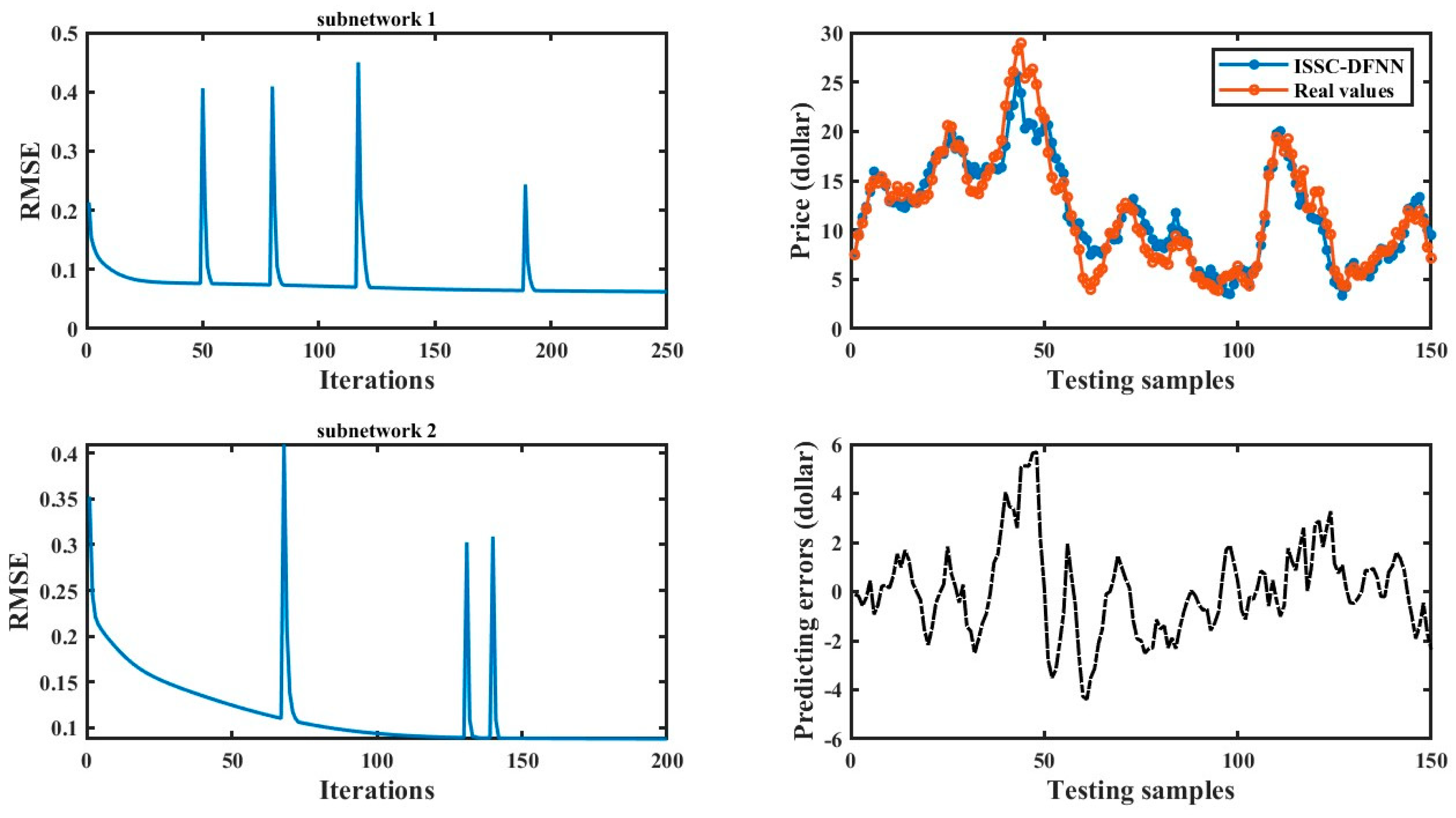
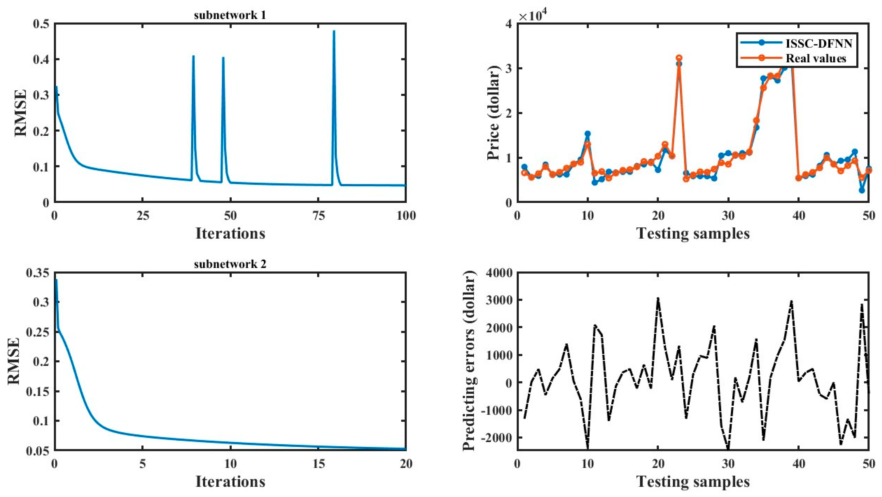
Figure 3. Training and testing results of Auto Price.

C.: Prediction results on benchmark problems

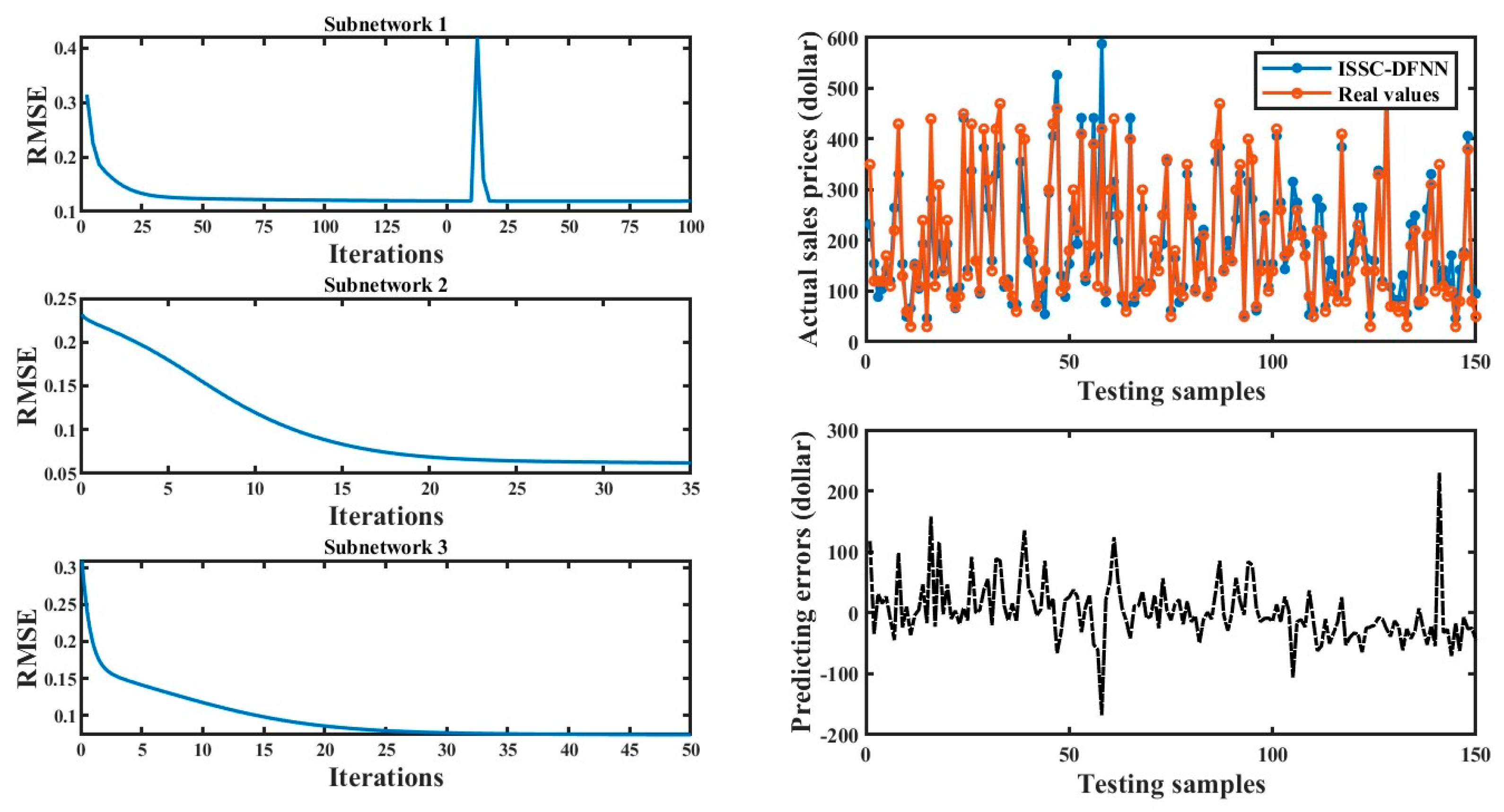
Figure 5 illustrate the training and testing results of ISSC-DFNN across different datasets. In each figure, the training RMSE curve gradually converges as the number of iterations increases, with noticeable jumps indicating the addition of hidden nodes within subnetworks to compensate for errors during training. The two subplots on the right display the testing outcomes of ISSC-DFNN, clearly demonstrating its strong approximation ability. Table 5 compares these results with several other models. Besides the evaluation metrics RMSE and MAPE, the number of subnetworks for each model is also reported to highlight structural advantages.

Figure 4. Training and testing results of Abalone.

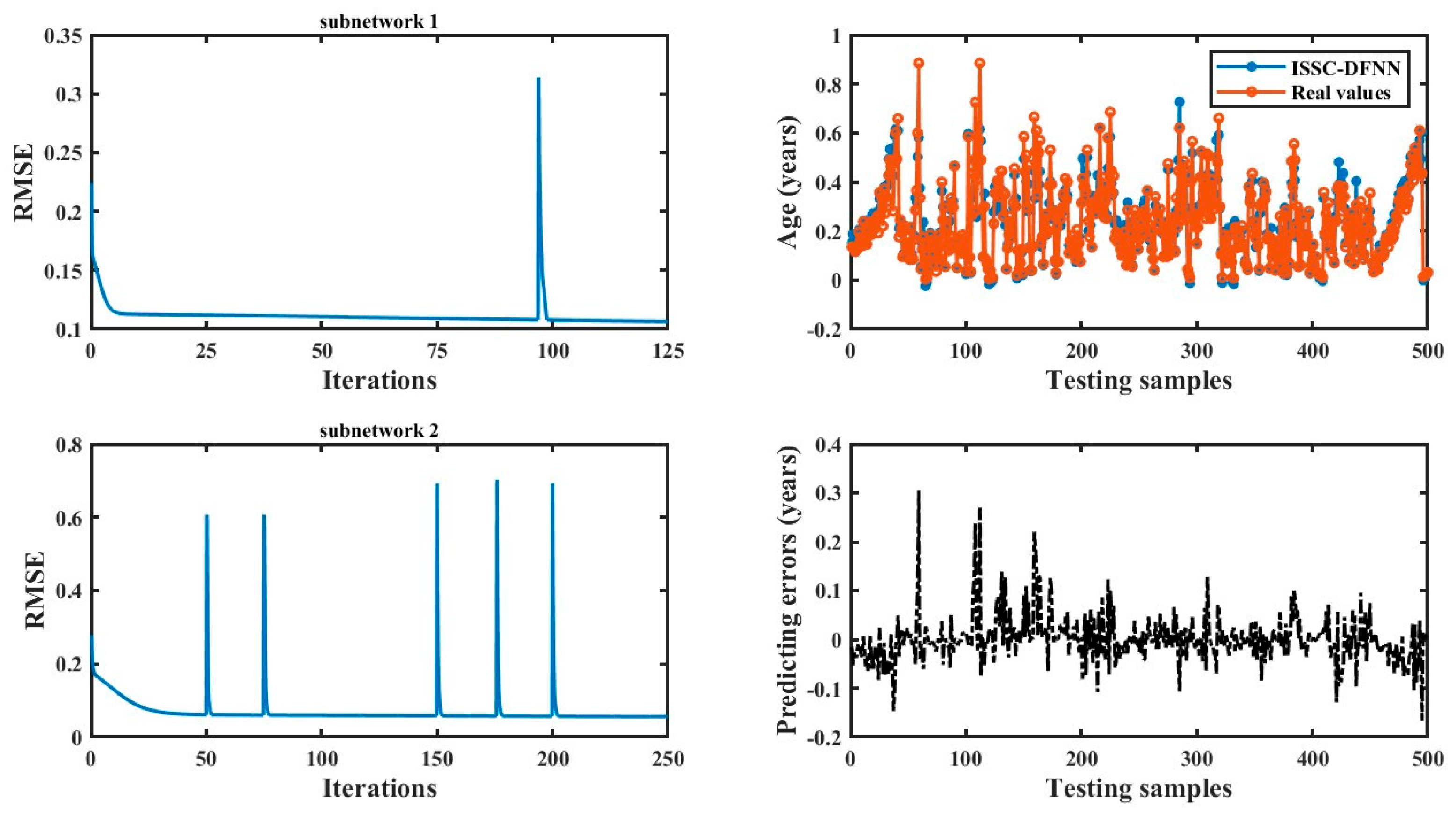
From Table 6, it is evident that ISSC-DFNN achieves the best performance across multiple metrics, followed by FC-AMNN, both utilize feature clustering methods. In contrast, OSAMNN and TMNN, which are based on sample clustering, exhibit comparatively weaker results. The primary distinction between ISSC-DFNN and FC-AMNN lies in their feature clustering approaches. Furthermore, ISSC-DFNN derives integration weights through task decomposition, making the task decomposition module more tightly coupled with the integration module, thereby enhancing overall model performance.

The relatively poorer performance of TMNN and OSAMNN can be attributed to several factors, including their sample decomposition strategies, subnetwork architectures, and integration weight calculation. Overall, soft-partition-based task decomposition demonstrates superior generalization ability, as reflected by the lower RMSE and MAPE values when comparing ISSC-DFNN to FC-AMNN. Additionally, ISSC-DFNN overcomes the issue of ineffective subnetwork training caused by insufficient samples in certain subtasks, a problem observed in TMNN and OSAMNN. Notably, ISSC-DFNN features a more compact architecture with fewer subnetworks, implying that it requires a smaller number of subnetworks to achieve the desired accuracy.

Figure 4. Training and testing results of Resident building.

D.: Results on ETP in wastewater treatment prediction

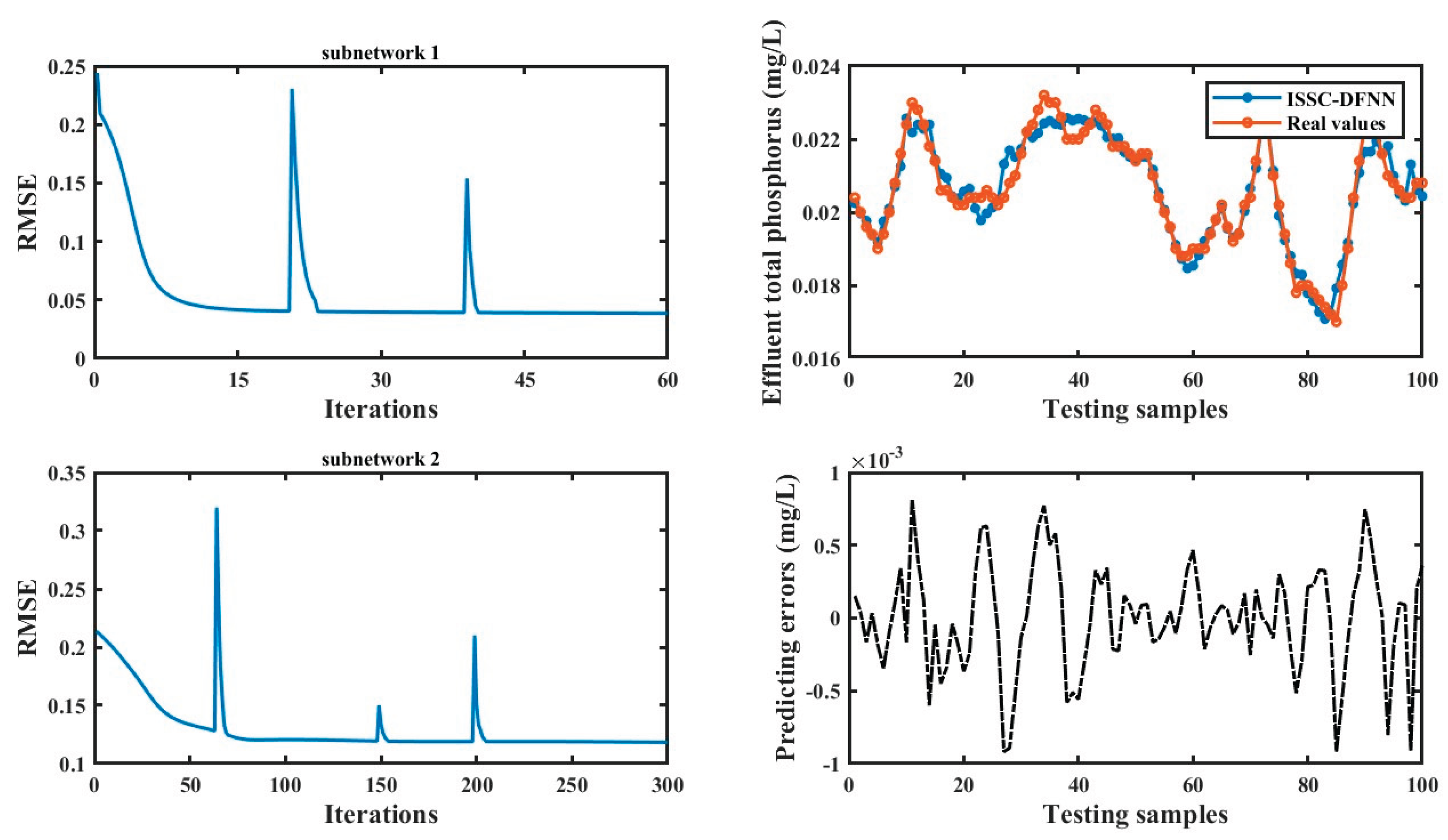
Figure 5 illustrates the testing results of ISSC-DFNN for a single trial on the effluent ETP dataset. As shown, ISSC-DFNN effectively captures the practical data trends, with the fitting curve demonstrating strong approximation capabilities. Table 6 presents the averaged prediction results of ISSC-DFNN alongside several other models over 20 trials for ETP concentration. It is evident from Table 6 that the predictions align well with benchmark outcomes. Similarly, ISSC-DFNN and FC-AMNN, which utilize a feature decomposition approach, outperform other methods on the practical dataset, followed by OSAMNN and TMNN that employ sample decomposition techniques. Notably, both training and testing RMSE values of ISSC-DFNN are lower than those of the competing models, indicating superior generalization performance. Additionally, as reflected in Table 6, ISSC-DFNN maintains a relatively simple architecture with a limited number of subnetworks.

Figure 5. Training and testing results of ETP concentration.

E.: Statistical analysis

To further demonstrate the superiority of the proposed model, we conducted a Wilcoxon signed-rank test (Demˇsar, 2006) to compare the performance of ISSC-DFNN with that of several baseline models. The Wilcoxon signed-rank test begins by computing the differences in evaluation metrics between two methods, followed by calculating the rank sums of the positive and negative differences, denoted as R⁺ and R^-, respectively. A significant difference is concluded if the resulting probability Pwilconxon value is less than the significance level 0.05. In this study, the testing RMSE is employed as the evaluation metric for all models.

Table 7 presents the results of the Wilcoxon signed-rank test. The experimental results indicate that, regardless of the comparison method, the ISSC-DFNN consistently satisfies the significance criterion of P_wilconxon <0.05. This confirms that the performance of the proposed ISSC-DFNN model is statistically significantly different from that of the other models, thereby further demonstrating its superiority.

VI. Conclusion

In this study, a distributed neural network framework is proposed, which is built upon the ISSC algorithm. The ISSC algorithm is utilized to perform feature clustering, thereby generating multiple subtasks with partially overlapping feature sets. Each subtask is handled by an RBF neural network trained using a self-organizing approach. Finally, the overall output is obtained by aggregating the predictions of all subnetworks using integration weights derived from the ISSC algorithm. The effectiveness of the proposed ISSC-DFNN has been confirmed by some simulated and experimental results. Table 5, Table 6 and Table 7 indicate that the proposed ISSC-DFNN achieved better testing RMSE, testing APE, and mean accuracy than the other algorithms. Based on experimental results, the characteristics of ISSC-DFNN are discussed and summarized as follows:

1) When confronted with large-scale datasets, the model is always able to acquire a leaner and denser feature representation, ensuring that each subtask preserves more input information to improve model accuracy.

2) The number of subnetworks can be kept small, even when dealing with datasets of very high dimensionality. Furthermore, based on the self-organizing strategy, each subnet can obtain a relatively compact structure in different subtasks, which is helpful to avoid redundant parameter training and reduce computational complexity.

3) The convergence of the proposed ISSC-DFNN can be maintained, and this proposed ISSC-DFNN with a comprehensive loss function may improve the chance of approximating the global optimization parameters.

Nevertheless, the proposed method still has certain limitations. One notable issue is the reliance on a large number of manually set parameters, including those within the ISSC algorithm as well as the parameters involved in subnetwork training. To address this, future work will focus on developing a more streamlined model with reduced parameter dependency.

Acknowledgments

The authors would like to thank you for reading the manuscript and providing valuable comments. The authors would also like to thank the anonymous reviewers for their valuable comments and suggestions, which helped improve this paper greatly.

References

Lin, F.J.; Sun, I.F.; Yang, K.J.; Chang, J.K. Recurrent fuzzy neural cerebellar model articulation network fault-tolerant control of six-phase permanent magnet synchronous motor position servo drive. IEEE Transactions on Fuzzy Systems 2016, 24, 153–167. [Google Scholar] [CrossRef]
Liu, Y.T.; Lin, Y.Y.; Wu, S.L.; Chuang, C.H.; Lin, C.T. Brain dynamics in predicting driving fatigue using a recurrent self-evolving fuzzy neural network. IEEE Transactions on Neural Networks and Learning System 2016, 27, 347–360. [Google Scholar] [CrossRef]
Zheng, Y.J.; Ling, H.F.; Chen, S.Y.; Xue, J.Y. A hybrid neuro-fuzzy network based on differential biogeography-based optimization for online population classification in earthquakes. IEEE Transactions on Fuzzy Systems 2015, 23, 1070–1083. [Google Scholar] [CrossRef]
Mohammed, M.F.; Lim, C.P. An enhanced fuzzy Min–Max neural network for pattern classification. IEEE Transactions on Neural Networks and Learning Systems 2015, 26, 417–429. [Google Scholar] [CrossRef]
Wai, R.J.; Chen, M.W.; Liu, Y.K. Design of adaptive control and fuzzy neural network control for single-stage boost inverter. IEEE Transactions on Industrial Electronics 2015, 62, 5434–5445. [Google Scholar] [CrossRef]
Ganjefar, S.; Tofighi, M. Single-hidden-layer fuzzy recurrent wavelet neural network: Applications to function approximation and system identification. Information Sciences 2015, 294, 269–285. [Google Scholar] [CrossRef]
Tofighi, M.; Alizadeh, M.; Ganjefar, S.; Alizadeh, M. Direct adaptive power system stabilizer design using fuzzy wavelet neural network with self-recurrent consequent part. Applied Soft Computing 2015, 28, 514–526. [Google Scholar] [CrossRef]
Rakkiyappan, R.; Balasubramaniam, P. On exponential stability results for fuzzy impulsive neural networks. Fuzzy Sets and Systems 2010, 161, 1823–1835. [Google Scholar] [CrossRef]
Huang, H.; Wu, C. Approximation of fuzzy functions by regular fuzzy neural networks. Fuzzy Sets and Systems 2011, 177, 60–79. [Google Scholar] [CrossRef]
Wai, R.J.; Chen, M.W.; Liu, Y.K. Design of adaptive control and fuzzy neural network control for single-stage boost inverter. IEEE Transactions on Industrial Electronics 2015, 62, 5434–5445. [Google Scholar] [CrossRef]
Coyle, D.; Prasad, G.; McGinnity, T.M. Faster self-organizing fuzzy neural network training and a hyperparameter analysis for a brain–computer interface. IEEE Transactions on Systems, Man, and Cybernetics, Part B: Cybernetics 2009, 39, 1458–1471. [Google Scholar] [CrossRef] [PubMed]
Vanualailai, J.; Nakagiri, S. Some generalized sufficient convergence criteria for nonlinear continuous neural networks. Neural computation 2005, 17, 1820–1835. [Google Scholar] [CrossRef] [PubMed]
Wu, W.; Li, L.; Yang, J.; Liu, Y. A modified gradient-based neuro-fuzzy learning algorithm and its convergence. Information Sciences 2010, 180, 1630–1642. [Google Scholar] [CrossRef]
Davanipoor, M.; Zekri, M.; Sheikholeslam, F. Fuzzy wavelet neural network with an accelerated hybrid learning algorithm. IEEE Transactions on Fuzzy Systems 2012, 20, 463–470. [Google Scholar] [CrossRef]
Lee, C.H.; Li, C.T.; Chang, F.Y. A species-based improved electromagnetism-like mechanism algorithm for TSK-type interval-valued neural fuzzy system optimization. Fuzzy Sets and Systems 2011, 171, 22–43. [Google Scholar] [CrossRef]
Ma, C.; Jiang, L. Some research on Levenberg–Marquardt method for the nonlinear equations. Applied Mathematics and Computation 2007, 184, 1032–1040. [Google Scholar] [CrossRef]
Kaminski, M.; Orlowska-Kowalska, T. An online trained neural controller with a fuzzy learning rate of the Levenberg–Marquardt algorithm for speed control of an electrical drive with an elastic joint. Applied Soft Computing 2015, 32, 509–517. [Google Scholar] [CrossRef]
Yang, Y.K.; Sun, T.Y.; Huo, C.L.; Yu, Y.H.; Liu, C.C.; Tsai, C.H. A novel self-constructing radial basis function neural-fuzzy system. Applied Soft Computing 2013, 13, 2390–2409. [Google Scholar] [CrossRef]
Ampazis, N.; Perantonis, S.J. Two highly efficient second-order algorithms for training feedforward networks. IEEE Transactions on Neural Networks 2002, 13, 1064–1074. [Google Scholar] [CrossRef]
Zhao, W.; Li, K.; Irwin, G.W. A new gradient descent approach for local learning of fuzzy neural models. IEEE Transactions on Fuzzy Systems 2013, 21, 30–44. [Google Scholar] [CrossRef]
Chen, C.L.P.; Wang, J.; Wang, C.H.; Chen, L. A new learning algorithm for a fully connected neuro-fuzzy inference system. IEEE Transactions on Neural Networks and Learning Systems 2014, 25, 1741–1757. [Google Scholar] [CrossRef] [PubMed]
Tzeng, S.T. Design of fuzzy wavelet neural networks using the GA approach for function approximation and system identification. Fuzzy sets and systems 2010, 161, 2585–2596. [Google Scholar] [CrossRef]
Kuo, R.J.; Hung, S.Y.; Cheng, W.C. Application of an optimization artificial immune network and particle swarm optimization-based fuzzy neural network to an RFID-based positioning system. Information Sciences 2014, 262, 78–98. [Google Scholar] [CrossRef]
Mashinchi, M.R.; Selamat, A. An improvement on genetic-based learning method for fuzzy artificial neural networks. Applied Soft Computing 2009, 9, 1208–1216. [Google Scholar] [CrossRef]
Chen, C.H.; Lin, C.J.; Lin, C.T. Nonlinear system control using adaptive neural fuzzy networks based on a modified differential evolution. IEEE Transactions on Systems, Man, and Cybernetics, Part C: Applications and Reviews 2009, 39, 459–473. [Google Scholar] [CrossRef]
Han, H.G.; Wu, X.L.; Qiao, J.F. Nonlinear systems modeling based on self-organizing fuzzy-neural-network with adaptive computation algorithm. IEEE Transactions on Cybernetics 2014, 44, 554–564. [Google Scholar] [CrossRef]
Miranian, A.; Abdollahzade, M. Developing a local least-squares support vector machines-based neuro-fuzzy model for nonlinear and chaotic time series prediction. IEEE Transactions on Neural Networks and Learning Systems 2013, 24, 207–218. [Google Scholar] [CrossRef]
Yu, H.; Reiner, P.D.; Xie, T.; Bartczak, T.; Wilamowski, B.M. An incremental design of radial basis function networks. IEEE Transactions on Neural Networks and Learning Systems 2014, 25, 1793–1803. [Google Scholar] [CrossRef]
Wu, S.; Er, M.J.; Gao, Y. A fast approach for automatic generation of fuzzy rules by generalized dynamic fuzzy neural networks. IEEE Transactions on Fuzzy Systems 2001, 9, 578–594. [Google Scholar]
Wu, S.; Er, M.J. Dynamic fuzzy neural networks-a novel approach to function approximation. IEEE Transactions on Systems, Man, and Cybernetics, Part B: Cybernetics 2000, 30, 358–364. [Google Scholar]
Teslic, L.; Hartmann, B.; Nelles, O.; Skrjanc, I. Nonlinear system identification by Gustafson–Kessel fuzzy clustering and supervised local model network learning for the drug absorption spectra process. IEEE Transactions on Neural Networks 2011, 22, 1941–1951. [Google Scholar] [CrossRef] [PubMed]
Wang, N.; Er, M.J.; Meng, X. A fast and accurate online self-organizing scheme for parsimonious fuzzy neural networks. Neurocomputing 2009, 72, 3818–3829. [Google Scholar] [CrossRef]
Rubio, J.J. SOFMLS: online self-organizing fuzzy modified least-squares network. IEEE Transactions on Fuzzy Systems 2009, 17, 1296–1309. [Google Scholar] [CrossRef]
Han, H.G.; Qiao, J.F. A self-organizing fuzzy neural network based on a growing-and-pruning algorithm. IEEE Transactions on Fuzzy Systems 2010, 18, 1129–1143. [Google Scholar] [CrossRef]
Zhang, L.; Li, K.; He, H.; Irwin, G.W. A new discrete-continuous algorithm for radial basis function networks construction. IEEE Transactions on Neural Networks and Learning Systems 2013, 24, 1785–1798. [Google Scholar] [CrossRef]
Lee, C.H.; Lee, Y.C. Nonlinear systems design by a novel fuzzy neural system via hybridization of electromagnetism-like mechanism and particle swarm optimisation algorithms. Information Sciences 2012, 186, 59–72. [Google Scholar] [CrossRef]
Oh, S.K.; Kim, W.D.; Pedrycz, W.; Seo, K. “Fuzzy radial basis function neural networks with information granulation and its parallel genetic optimization. Fuzzy Sets and Systems 2014, 237, 96–117. [Google Scholar] [CrossRef]
Juang, C.F.; Cheng, W.; Liang, C. Speedup of learning in interval type-2 neural fuzzy systems through graphic processing units. IEEE Transactions on Fuzzy Systems 2015, 23, 1286–1298. [Google Scholar] [CrossRef]
Zhao, W.; Zhang, J.; Li, K. An efficient LS-SVM-based method for fuzzy system construction. IEEE Transactions on Fuzzy Systems 2015, 23, 627–643. [Google Scholar] [CrossRef]
Juang, C.F.; Lin, Y.Y.; Tu, C.C. A recurrent self-evolving fuzzy neural network with local feedbacks and its application to dynamic system processing. Fuzzy Sets and Systems 2010, 161, 2552–2568. [Google Scholar] [CrossRef]
Wang, N.; Er, M.J.; Han, M. Dynamic tanker steering control using generalized ellipsoidal- basis-function-based fuzzy neural networks. IEEE Transactions on Fuzzy Systems 2015, 23, 1414–1427. [Google Scholar] [CrossRef]
Tonidandel, S.; Lebreton, J.M. Relative importance analysis: a useful supplement to regression analysis. Journal of Business & Psychology 2011, 26, 1–9. [Google Scholar]
Chao, Y.C.E.; Zhao, Y.; Kupper, L.L.; Nylander-French, L.A. “Quantifying the relative importance of predictors in multiple linear regression analyses for public health studies. Journal of Occupational & Environmental Hygiene 2008, 5, 519–529. [Google Scholar]
Gacek, A.; Pedrycz, W. Clustering granular data and their characterization with information granules of higher type. IEEE Transactions on Fuzzy Systems 2015, 23, 850–860. [Google Scholar] [CrossRef]
K. M.; Sim; Guo, Y.; Shi, B. BLGAN: Bayesian learning and genetic algorithm for supporting negotiation with incomplete information. IEEE Transactions on Systems, Man and Cybernetics, Part B: Cybernetics 2009, 39, 198–211. [Google Scholar] [CrossRef] [PubMed]
Chen, H.; Gong, Y.; Hong, X. Online modeling with tunable RBF network. IEEE Transactions on Cybernetics 2013, 43, 935–947. [Google Scholar] [CrossRef] [PubMed]
Zubrowska-Sudol, M.; Walczak, J. Enhancing combined biological nitrogen and phosphorus removal from wastewater by applying mechanically disintegrated excess sludge. Water Research 2015, 76, 10–18. [Google Scholar] [CrossRef]
Sicard, C.; Glen, C.; Aubie, B.; Wallace, D.; Jahanshahi-Anbuhi, S.; Pennings, K.; Daigger, G.T.; Pelton, R.; Brennan, J.D.; Filipe, C.D.M. Tools for water quality monitoring and mapping using paper-based sensors and cell phones. Water Research 2015, 70, 360–369. [Google Scholar] [CrossRef]
Winkler, M.K.; Ettwig, K.F.; Vannecke, T.P.; Stultiens, K.; Bogdan, A.; Kartal, B.; Volcke, E.I.P. Modelling simultaneous anaerobic methane and ammonium removal in a granular sludge reactor. Water Research 2015, 73, 323–331. [Google Scholar] [CrossRef]
Gujer, W. Nitrification and me-A subjective review. Water Research 2010, 44, 1–19. [Google Scholar] [CrossRef]
Kaelin, D.; Manser, R.; Rieger, L.; Eugster, J.; Rottermann, K.; Siegrist, H. Extension of ASM3 for two-step nitrification and denitrification and its calibration and validation with batch tests and pilot scale data. Water Research 2009, 43, 1680–1692. [Google Scholar] [CrossRef] [PubMed]

Figure 1. Structure of ISSC-DNN.

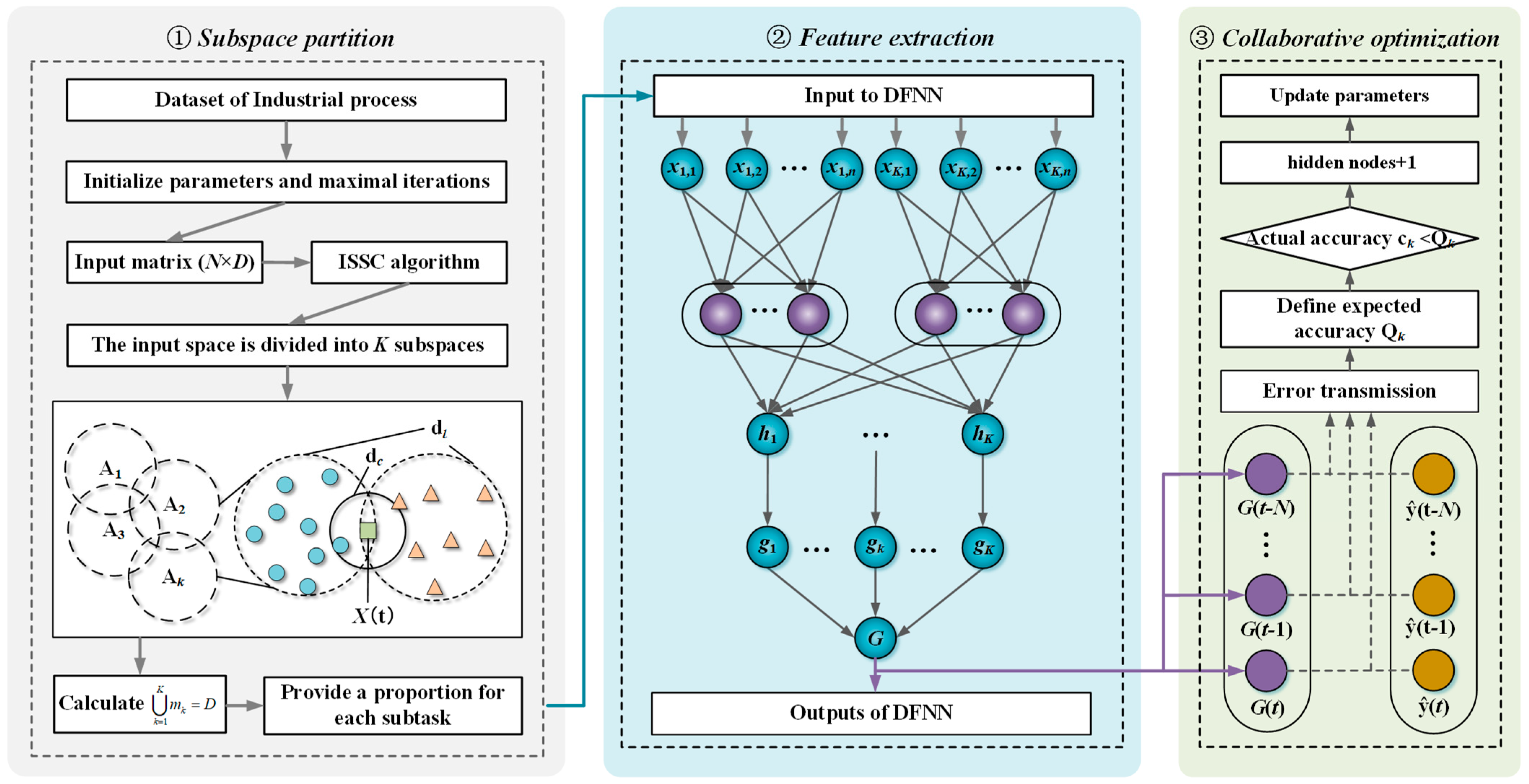
Table 1. The ISSC based feature partitioning algorithm.

1: C=1
2: Initialize the parameters and set the maximum number of iterations to Max.
3: Repeat:
4: C=C+1;
5: Arbitrarily initialize cluster centers matrix V(0), initialize the weight matrix W(0).
6: Repeat: iter = iter + 1;
7: Calculate the membership matrix U(iter) according to Eq. (4);
8: Calculate the weight matrix W(iter) according to Eq. (6);
9: Until ||V(iter)-V(iter-1)||<ζ or iter = Max.
10: Calculate the JIESSC by Eq. (2);
11: Until C = 2log(D); D is the number of input features.
12: Calculate the minimum value of J and the optimal clusters K.

Table 3. Information for FOUR UCI datasets.

Dataset	Training samples	Testing samples	Input dimensions	Output dimension
Boston Housing	350	150	13	1
Auto Price	120	50	14	1
Abalone	1500	500	8	1
Residential building	350	150	107	1

Table 4. Input variables of ETP dataset.

X₁	Inlet flow	X₁₃	BOD
X₂	Temperature	X₁₄	Influent oil
X₃	ORP1	X₁₅	Effluent oil
X₄	ORP2	X₁₆	Influent ammonia
X₅	MLSS1	X₁₇	Influent colourity
X₆	NO3-N	X₁₈	Effluent colourity
X₇	NH4-N	X₁₉	Influent PH
X₈	DO₁	X₂₀	Effluent PH
X₉	ORP₃	X₂₁	Suspended Solid
X₁₀	MLSS₂	X₂₂	Influent nitrogen
X₁₁	NO3-N	X₂₃	Influent phosphate
X₁₂	DO₂	Y_d	ETP

Table 5. Comparison results with other models for UCI benchmark problems.

Algorithm	Dataset A: Boston Housing				Dataset B: Auto Price
Algorithm	Training RMSE	Testing RMSE	Testing APE	Subnetworks	Training RMSE	Testing RMSE	Testing APE	Subnetworks
Prop.	0.0759	0.0741	0.1375	2	0.0738	0.0742	0.1729	2
FC-AMNN	0.0767	0.0748	0.1396	4	0.0752	0.0766	0.1781	2
TMNN	0.0875	0.0906	0.1684	2	0.0872	0.0883	0.1968	2
OSAMNN	0.0927	0.1006	0.1734	8	0.0785	0.0810	0.1892	5
Algorithm	Dataset C: Abalone				Dataset D: Residential building
Algorithm	Training RMSE	Testing RMSE	Testing APE	Subnetworks	Training RMSE	Testing RMSE	Testing APE	Subnetworks
Prop.	0.0739	0.0741	0.1721	2	0.0987	0.0962	0.467	3
FC-AMNN	0.0774	0.0786	0.1797	2	0.0994	0.1062	0.4963	4
TMNN	0.0823	0.0886	0.1895	2	0.1152	0.1204	0.5397	3
OSAMNN	0.0815	0.0879	0.1838	7	0.1074	0.1126	0.5124	4

Table 6. Comparison results with other models on ETP.

Algorithm	Training RMSE	Testing RMSE	Testing APE	Subnetwork
Prop.	0.0763	0.0781	0.0306	2
FC-AMNN	0.0802	0.0816	0.0391	2
TMNN	0.0984	0.0996	0.0502	3
OSAMNN	0.0795	0.0828	0.0412	7

Table 7. Wilcoxon’s test results of Testing RMSE on all datasets.

Models	R⁺	R^-	P_wilconxon
Prof. vs TMNN	21	0	0.00741
Prof. vs FC-AMNN	21	0	0.00741
Prof. vs OSAMNN	21	0	0.00741

Disclaimer/Publisher’s Note: The statements, opinions and data contained in all publications are solely those of the individual author(s) and contributor(s) and not of MDPI and/or the editor(s). MDPI and/or the editor(s) disclaim responsibility for any injury to people or property resulting from any ideas, methods, instructions or products referred to in the content.

© 2025 by the authors. Licensee MDPI, Basel, Switzerland. This article is an open access article distributed under the terms and conditions of the Creative Commons Attribution (CC BY) license (http://creativecommons.org/licenses/by/4.0/).

Copyright: This open access article is published under a Creative Commons CC BY 4.0 license, which permit the free download, distribution, and reuse, provided that the author and preprint are cited in any reuse.