
Submitted:
02 July 2025
Posted:
03 July 2025
You are already at the latest version
Abstract
Economic freedom is generally regarded as a driver of growth; however, its impact on economies that have recently transitioned remains unclear. In the Western Balkans, a region characterised by institutional instability and inconsistent market reforms, the influence of economic freedom on long-term economic outcomes necessitates more rigorous empirical examination. This study analyses the impact of five critical dimen-sions of economic freedom: Property Rights, Government Integrity, Government Spending, Business Freedom, and Monetary Freedom on GDP per capita growth in six Western Balkan countries from 2013 to 2023. The study utilises a triangulated analytical strategy, employing the Generalised Method of Moments (GMM) to mitigate endoge-neity, Bayesian Vector Autoregression (VAR) to elucidate dynamic interdependencies, and Random Forest regression to identify non-linearities and prioritise predictor sig-nificance. The GMM findings demonstrate that Property Rights and Monetary Freedom positively and significantly impact economic growth, whereas Government Spending has a detrimental effect. Surprisingly, Government Integrity has a negative relationship with growth, which could be due to problems with transitional governance. Bayesian VAR shows that GDP dynamics are very stable over time, but it doesn't find that EF indicators have any immediate effects. Random Forest analysis shows that Government Spending, Business Freedom, and Property Rights are the most important variables. This is because it finds non-linear and interactive patterns that other models don't. Economic freedom is a significant, albeit contextually variable, factor influencing growth in the Western Balkans. The results indicate that focused institutional reforms, especially those that improve property rights, make public spending more efficient, and lower regulatory barriers, can help the economy do well over time. For the region to grow in the long term, it needs a hybrid policy that combines opening up the market with strengthening governance.
Keywords:
Economic Freedom
; GDP Growth
; Generalised Method of Moments (GMM)
; Bayesian Vector Autoregression (VAR)
; Random Forest
0. How to Use This Template
The template details the sections that can be used in a manuscript. Note that each section has a corresponding style, which can be found in the “Styles” menu of Word. Sections that are not mandatory are listed as such. The section titles given are for articles. Review papers and other article types have a more flexible structure.
Remove this paragraph and start section numbering with 1. For any questions, please contact the editorial office of the journal or support@mdpi.com.
1. Introduction
There has been a long-standing debate in economic literature about the link between economic freedom (EF) and economic growth (EG). This debate has led to a range of empirical conclusions. Initial research, including works by Ali (1997), Easton and Walker (1997), Goldsmith (1997), Dawson (1998), Wu and Davis (1999), and Hanson (2000), indicates a favourable correlation between economic freedom and economic performance. Heckelman (2000) observes that enhancements in economic liberalisation are often associated with improved economic results. However, later contributions show effects that are less strong or more conditional. For example, Gwartney et al. (2002), Gwartney, Lawson, and Holcombe (1998), and De Haan and Sturm (2000) only find a weak positive link, while Pitlik (2002) says that the direction of change in EF is more important than its level. Weede and Kampf (2002) corroborate this nuanced perspective by demonstrating that alterations in economic freedom, rather than its absolute level, influence economic growth.
As a concept, EF includes a lot of different things, such as the protection of property rights, the integrity of institutions, the size of government, market openness, and monetary stability. These dimensions together make up the business environment and affect how well people and businesses can do useful economic work (Hussain, 2016). Still, the link between EF and EG is still complicated. Al-Gasaymeh et al. (2020) and Chang et al. (2020) assert that EF facilitates the advancement of the financial system by mitigating inefficiencies and refining financial procedures. Conversely, Kacprzyk (2016) and Slesman, Baharumshah, and Azman-Saini (2019) recognise that these outcomes are contingent upon contextual factors, including governance quality, transparency, and institutional maturity.
This complexity is especially evident in the Western Balkan region. Even though these countries, Albania, Bosnia and Herzegovina, Croatia, Kosovo, Montenegro, and Serbia have seen some moderate growth over the past ten years, they still have problems with weak institutions, high levels of corruption, wasteful public spending, a lack of job opportunities, and structural mismatches (Uvalić & Cvijanović, 2018). The potential advantages of EF are recognised; however, their implementation frequently faces challenges due to institutional fragility, rent-seeking behaviour, and policy inconsistency (Farah et al., 2021; Fang & Zhang, 2016).
In light of these tensions, this study re-examines the EF–EG relationship within the Western Balkan context, utilising recent data from 2013 to 2023. Five principal subcomponents of economic freedom, Property Rights (PR), Government Integrity (GI), Government Spending (GS), Business Freedom (BF), and Monetary Freedom (MF) are analysed for their impact on GDP per capita growth. This study utilises a triangulated econometric strategy, incorporating the Generalised Method of Moments (GMM), Bayesian Vector Autoregression (Bayesian VAR), and Random Forest (RF) techniques, in contrast to previous research that primarily concentrated on linear models or global datasets. This multifaceted approach facilitates the identification of both dynamic and non-linear effects, providing a more nuanced comprehension of the EF–EG nexus.
The study contributes to the literature in three key ways. First, it provides updated and region-specific empirical evidence from the Western Balkans, an area often underrepresented in mainstream EF research. Second, it adopts a dynamic GMM model to correct for endogeneity and omitted variable bias, building on the methodological gap identified by Rachdi, Hakimi and Hamdi (2015) and Aldiabat, Al-Gasaymeh and Rashid (2019). Third, it leverages machine learning to assess variable importance and uncover patterns not readily captured by parametric models.
Hypothesis:
Null Hypothesis (H0): There is no significant relationship between Economic Freedom (EF) and Economic Growth (EG) in Western Balkan countries.
Alternative Hypothesis (H1): There is a significant positive relationship between Economic Freedom (EF) and Economic Growth (EG) in Western Balkan countries.
2. Literature Review
There is still a great deal of disagreement among academics regarding the connection between economic growth (EG) and economic freedom (EF). Although the fundamental perspective, which was advanced by Ali (1997), Easton and Walker (1997), and Dawson (1998), contends that increased economic freedom promotes higher growth by decreasing government intervention, increasing efficiency, and stimulating private initiative, this consensus has been steadily eroding. For example, De Haan and Sturm (2000) and Gwartney, Lawson, and Holcombe (1998) only find weak or context-dependent relationships between EF and long-term growth. In a similar vein, Adkins, Moomaw, and Savvides (2002) point out that the institutional quality supporting EF may have an impact on how effective monetary policy is.
Weede and Kampf (2002) offer a more nuanced critique, contending that the direction of change, rather than the degree of economic freedom, determines growth. In line with this, Berggren (2003) points out that some aspects of EF, like human development, institutional transparency, and income equality, might be more important than overall freedom indices. Thuy (2022) supports this argument by demonstrating that while changes in EF can have important macroeconomic repercussions, static EF levels do not always result in growth.
The notion that EF functions independently is still being contested by recent research. Higher levels of corruption reduce the anticipated benefits of EF by discouraging foreign investment and warping resource allocation, according to Okunlola and Akinlo's (2021) analysis of the mediating role of corruption. According to Mo (2001), corruption also hinders political stability and the development of human capital, two important channels via which EF is supposed to promote growth. Similar to this, Herrera-Echeverri, Haar, and Estévez-Bretón (2014) show that weak governance frameworks limit EF's ability to boost growth, especially in developing nations.
Additional texture is provided by regional viewpoints. Government size and growth are positively correlated in Western Balkan nations, according to Bajrami (2022), which implies that state participation, which is sometimes seen as counterproductive to EF, can occasionally boost growth in situations where institutional capacities are constrained. The significance of trade openness as a conduit for EF's contribution to economic growth is emphasised by Bajraktari (2023). However, Puška, Štilić, and Stojanović (2023) warn that regional EF rankings could conceal more serious institutional flaws like pervasive cronyism and lax regulatory enforcement.
In a broader sense, international research supports the EF–EG nexus' complexity. EF only improves quality of life when stable governance is present, according to Akinlo and Okunlola (2025), who take political risk factors into account in their African context. Using bibliometrics, Sharma (2025) notes that recent research trends are shifting away from the neoliberal orthodoxy that formerly dominated the EF literature and towards an increased emphasis on institutional quality and social outcomes. Financial deregulation, which is frequently seen as a sign of economic freedom, can, in some circumstances, jeopardise financial stability, according to Duan et al. (2025).
The degree to which economic freedom measures are consistent across nations is questioned by Payne et al. (2025) in terms of convergence and global trends. They contend that although some EF principles have been harmonised as a result of globalisation, national-level quirks like political cycles, legal traditions, and regulatory cultures still lead to different results. A similar tension is revealed by Canale and Liotti (2025), who concentrate on the Eurozone. An overly minimalist state runs the risk of undermining the social compact, even though economic freedom may help alleviate poverty, particularly in economies that are already fragile.
Brkić, Gradojević, and Ignjatijević's (2020) empirical work is particularly pertinent to this investigation. In their analysis of 28 EU nations, they discover that EG is positively correlated with a number of EF sub-dimensions, particularly through financial development: property rights, fiscal policy discipline, trade openness, and administrative efficiency. By addressing endogeneity issues with the GMM estimator, this study offers a convincing methodological precedent. The authors leave room for methodological development, though, by not utilising machine learning or dynamic forecasting techniques.
Last but not least, Gehring (2013), Verner (2015), and Hussain and Haque (2016) all provide additional evidence for the EF-growth link, albeit through distinct avenues, ranging from the accumulation of tangible capital to institutional legitimacy and subjective well-being. The variety of these results highlights the significance of contextual specificity as well as the multifaceted nature of economic freedom. Recent studies have further enriched this discourse in the context of the Western Balkans. Bajraktari, Bajrami, and Hashani (2023) explored the link between international trade freedom and growth, identifying external openness as a key amplifier of domestic economic performance. Bajrami et al. (2025) provide fresh evidence on the role of money supply in the region's growth process, highlighting the monetary channel's strategic importance in post-transition economies. Similarly, Gashi, Tafa, and Bajrami (2022) analyse macroeconomic determinants of non-performing loans, reinforcing the link between institutional stability and financial health. Hoxha, Bajrami, and Prekazi (2025) assess how both internal banking and macroeconomic factors shape profitability in the regional banking sector, suggesting that economic and institutional reforms must be considered in tandem to sustain growth. These contributions collectively underscore the interconnectedness between financial discipline, regulatory reform, and growth outcomes in the Western Balkans.
In conclusion, three significant gaps are revealed. First, post-transition areas like the Western Balkans receive comparatively little attention in the empirical literature, which is still largely centred on advanced economies. Secondly, current research frequently uses static models that are unable to adequately represent the dynamic or lagged effects of EF. Third, very few analyses use machine learning techniques to find interaction effects or non-linearities. Using GMM, Bayesian VAR, and Random Forest models to analyse disaggregated EF indicators across six Western Balkan nations, this study fills these gaps while offering both methodological innovation and regional relevance.

Table 1.
Empirical Findings .
| AUTHOR | TIME AND REGIONAL SCOPE | RESULTS / EMPIRICAL FINDINGS |
| Işık et al. (2023) | 2023; G-7 and BRIC countries | Economic freedom positively influences renewable energy adoption, but economic policy uncertainty weakens this relationship. Higher economic freedom thresholds are necessary for the transition to renewable energy. |
| Puška, Štilić, & Stojanović (2023) | 2023; Balkan countries | Multi-criteria ranking reveals disparities in economic freedom across Balkan nations, with significant variation in institutional efficiency and regulatory frameworks. |
| Iskandar et al. (2023) | 2023; East Asia | Strong institutional frameworks contribute positively to economic growth, but their effectiveness varies depending on governance quality and stability. |
| de Haan & Sturm (2024) | 2024; Global analysis | Economic freedom is positively correlated with economic growth, though the strength of the relationship varies based on institutional contexts and policy environments. |
| Akinlo & Okunlola (2025) | 2025; Africa | Economic freedom enhances quality of life, but political risk factors can significantly undermine its benefits, suggesting the need for stable governance. |
| Sharma (2025) | 2025; Global bibliometric analysis | Economic freedom research has expanded over time, with emerging trends focusing on institutional quality, governance, and social implications. Future research should address methodological limitations and regional disparities. |
| Duan et al. (2025) | 2025; Various regions | Financial freedom moderates the impact of government intervention on financial stability, with excessive deregulation posing systemic risks. |
| Payne et al. (2025) | 2025; Cross-country analysis | Economic freedom convergence is influenced by institutional structures, globalization, and regulatory harmonization, though national differences persist. |
| Canale & Liotti (2025) | 2025; Eurozone | Economic freedom can reduce poverty, but an excessively small government may weaken social safety nets and public welfare. |
| Vodareva and Fifekova (2016) | 2000 - 2015 European Union countries |
Economic freedom creates better conditions for increasing economic performance. In this paper on the case of European countries, it has been shown that the most economically developed countries transform their high level of economic freedom into a higher economic level. |
| Juice (2017) | 2000 – 2013 Panel from 52 countries |
Reducing the size of government, strengthening the legal structure and property rights and maintaining a stable monetary policy (increasing access to sound money) has a positive effect on economic growth. |
| Katout (2019) | 2004 – 2017 Panel of 42 countries in the first group and 29 countries in the second group |
In the first group, the value of the relationship between GDP per capita and economic freedom is higher than in the second group, reaching 0.511 in the first group compared to 0.241 in the second group. Countries in the first group are characterized by high incomes and thus flexibility will tend to increase compared to countries in the second group, which have lower per capita incomes. |
| Bajrami (2022) | 2000 to 2017 Wester Balkan Country |
The findings reveal a positive relationship between government size and economic growth in the region, with a 1% increase in government size leading to a 0.29% rise in GDP per capita |
| Bajraktari (2023) | 2000 – 2021 Wester Balkan Country |
The empirical findings from the study on the Western Balkan countries reveal a strong positive relationship between international trade freedom and economic growth |
3. Materials and Methods
3.1. Research Design and Scope
This study investigates the impact of economic freedom (EF) on economic growth (EG) in six Western Balkan countries, Albania, Bosnia and Herzegovina, Croatia, Kosovo, Montenegro, and Serbia, over the period 2013 to 2023. To achieve this, a panel dataset is constructed using annual data covering five sub-dimensions of economic freedom: Property Rights (PR), Government Integrity (GI), Government Spending (GS), Business Freedom (BF), and Monetary Freedom (MF). The dependent variable is the annual growth rate of gross domestic product per capita (GDP), which serves as a proxy for economic growth.
Economic freedom indicators are sourced from the Heritage Foundation’s Index of Economic Freedom, while GDP growth data are obtained from the World Bank’s World Development Indicators (2023 edition). The model specification assumes that economic growth is a function of the selected EF sub-dimensions, which are treated as both contemporaneous and potentially lagged determinants.
The functional relationship is formalised as:
where:
: Economic growth (GDP per capita growth rate) for country at time ;
to : Sub-dimensions of economic freedom;
: Error term capturing unobserved shocks.
To robustly estimate this relationship, three complementary methodological approaches are employed: Generalised Method of Moments (GMM), Bayesian Vector Autoregression (Bayesian VAR), and Random Forest (RF) machine learning.
3.2. Generalised Method of Moments (GMM)
To account for potential endogeneity and omitted variable bias inherent in panel datasets, the study employs a dynamic GMM estimator, following the Arellano-Bond framework. GMM is particularly suitable in this context due to its capacity to control for unobserved heterogeneity and simultaneity bias, as well as its efficiency in the presence of autocorrelation and heteroskedasticity.
The model specification is expressed as:
where:
: One-period lag of GDP growth;
: Country-specific fixed effects;
: Idiosyncratic error term;
and : Parameters to be estimated.
A two-step system GMM estimator is used to enhance efficiency. The validity of instruments is assessed through the Sargan test for over-identifying restrictions, while Arellano-Bond tests for serial correlation in the residuals ( and ) are applied to ensure model consistency.
3.3. Machine Learning Approach: Random Forest Regression
To capture possible non-linearities and interaction effects overlooked by traditional econometric methods, the study incorporates a machine learning algorithm—Random Forest Regression. This ensemble method constructs a multitude of decision trees during training and outputs the average prediction, reducing overfitting and enhancing predictive accuracy.
Key steps include:
Feature Selection: Economic freedom sub-indicators are evaluated for importance using measures such as IncNodePurity, which reflects each variable’s contribution to model accuracy.
Model Training: A forest of 500 trees is trained using the EF indicators as predictors of GDP growth. A standard 70/30 train-test split is employed.
Cross-Validation: K-fold cross-validation (with ) is conducted to validate the model’s generalisability.
Interpretability: Variable importance rankings are derived, and SHAP (Shapley Additive Explanations) values are proposed for future interpretability enhancement.
Model performance is evaluated using Root Mean Squared Error (RMSE) and R-squared () metrics, providing insight into prediction accuracy and explanatory power.
Bayesian Vector Autoregression (Bayesian VAR)
To assess the dynamic interdependencies and delayed effects of economic freedom indicators on economic growth, a Bayesian Vector Autoregression (VAR) model is estimated. Bayesian VAR is particularly advantageous for small-sample studies, allowing for the inclusion of prior information to stabilise coefficient estimates.
The Bayesian VAR model is defined as:
where:
: A vector including GDP growth and the five EF indicators;
: Parameter matrices for lag ;
: Intercept vector;
: Vector of innovations.
This study employs the Litterman/Minnesota prior, which favours more weight on own lags and shrinks cross-variable influence. Impulse Response Functions (IRFs) are generated to trace the temporal effect of shocks in EF components on GDP growth. Additionally, the model’s fit is evaluated using the Adjusted R-squared, F-statistics, and the Standard Error of Regression.
3.4. Summary of Analytical Strategy
By combining GMM, Bayesian VAR, and Random Forest models, the analysis captures a comprehensive view of the EF–EG nexus. While GMM identifies causal and contemporaneous effects under endogeneity, Bayesian VAR models lag structures and dynamic feedback, and Random Forest allows for complex non-linear interactions and variable importance assessment. This triangulated approach enhances empirical validity and provides policy-relevant insights grounded in methodological pluralism.
4. Results
This section presents the empirical findings from the three methodological approaches employed Generalised Method of Moments (GMM), Bayesian Vector Autoregression (Bayesian VAR), and Random Forest (RF). The results offer a multi-dimensional understanding of how various subcomponents of economic freedom influence GDP per capita growth across six Western Balkan countries between 2013 and 2023.
4.1. Diagnostics for Pre-Estimation
Preliminary tests were performed to evaluate the time series properties of the variables in order to guarantee the validity and robustness of the econometric models used. The study used the Levin–Lin–Chu (LLC) and Im–Pesaran–Shin (IPS) panel unit root tests to confirm stationarity because of the panel structure (six countries over 11 years). The findings showed that while some economic freedom indicators and GDP growth were stationary at first difference, others were stationary at level.
The presence of long-term equilibrium relationships between the variables was also evaluated using the Pedroni panel cointegration test. Long-term relationships were included in the panel regression models due to evidence of cointegration, which helped to reduce the possibility of spurious regression, as warned by Granger and Newbold (1974) and Hamilton (1994).
In addition to validating the empirical approach, these pre-estimation checks offer a strong statistical basis for subsequent estimation using the Random Forest, Bayesian VAR, and GMM techniques.
Table 2.
Panel Unit Root Tests for Level and First Difference.
| Variable | Test | Statistic | p-value | Stationary |
| GDP Growth | LLC (Level) | –1.12 | 0.130 | No |
| IPS (1st Diff) | –3.85 | 0.0002 | Yes | |
| Property Rights | LLC (Level) | –0.94 | 0.173 | No |
| IPS (1st Diff) | –4.21 | 0.0000 | Yes | |
| Government Integrity | LLC (Level) | –0.88 | 0.191 | No |
| IPS (1st Diff) | –3.62 | 0.0003 | Yes | |
| Government Spending | LLC (Level) | –1.00 | 0.159 | No |
| IPS (1st Diff) | –4.07 | 0.0001 | Yes | |
| Business Freedom | LLC (Level) | –0.95 | 0.170 | No |
| IPS (1st Diff) | –3.97 | 0.0001 | Yes | |
| Monetary Freedom | LLC (Level) | –1.04 | 0.147 | No |
| IPS (1st Diff) | –4.11 | 0.0001 | Yes |
4.2. Descriptive Statistics
Table 3 presents the descriptive statistics for the dependent and independent variables over the period 2013–2023 for the six Western Balkan countries. On average, annual GDP per capita growth stood at 2.45%, with a standard deviation of 1.26%, indicating moderate variation across countries and time. Among the economic freedom indicators, Property Rights (PR) averaged 61.8, reflecting moderate institutional protection of ownership, while Government Integrity (GI) recorded a mean of 41.2, pointing to persistent governance challenges. Government Spending (GS) remained relatively high (mean = 29.4), while Business Freedom (BF) and Monetary Freedom (MF) were more favourable, averaging 66.3 and 70.1, respectively.
4.3. Correlation Matrix
Although the correlation matrix offers a summary of the pairwise relationships between the variables, it is important to interpret it carefully. Correlations between trending variables could be deceptive in the absence of stationarity. Formal unit root and cointegration tests were performed to address this, confirming that the variables are either cointegrated or stationary (see Section 4.1). This guarantees that there are no fictitious relationships represented in the correlation matrix.
The bivariate relationships between variables are displayed in Table 4's Pearson correlation matrix. Notably, government spending (GS) has a negative correlation with growth (r = -0.24), whereas property rights (PR) and monetary freedom (MF) show a modest positive correlation with GDP growth (r = 0.31 and 0.28, respectively). The independent variables' correlations are typically low, indicating little redundancy.
All correlations fall below the conventional multicollinearity threshold of 0.80, indicating no problematic linear dependence between regressors.
4.4. Multicollinearity Test (Variance Inflation Factor – VIF)
To further assess multicollinearity, Variance Inflation Factors (VIFs) were computed for all independent variables. As shown in Table 5, all VIF values fall below 3.0, well under the conservative threshold of 5.0, indicating no evidence of multicollinearity in the model.
These results confirm that the regression estimates presented earlier are not biased or inflated by collinearity among predictors.
4.5. Generalised Method of Moments (GMM) Estimates
The GMM model is estimated using a two-step system GMM framework to correct for endogeneity and unobserved heterogeneity. Table 6 summarises the coefficient estimates and statistical significance levels.
Model diagnostics:
AR(1) = -2.38 (p = 0.0173)
AR(2) = 2.17 (p = 0.0298)
Sargan test = χ²(38) = 115.91 (p < 0.0001)
Wald test = χ² = 6.19e+11 (p < 0.0001)
Note: p < 0.10 (***), p < 0.05 (**), p < 0.01 (*), NS = not significant
A number of significant dynamics are revealed by the GMM regression model (Table 6) in order to explain the growth of GDP per capita in the Western Balkan nations. A high degree of persistence in economic growth is indicated by the coefficient on the lagged dependent variable, GDP(-1), which is 0.9384 and highly statistically significant (p < 0.0001). According to dynamic growth models, this implies that past growth trajectories have a significant impact on present performance.
The model predicts a slightly negative GDP growth rate in the absence of other explanatory variables, as evidenced by the constant term, which is negative at -0.7116 and marginally significant at the 10% level (p = 0.0983). Although it anchors the model's baseline, the constant has little interpretive value in a model with differenced or lag terms.
Property Rights (PR) has a positive and statistically significant coefficient of 0.0367 (p = 0.0208) when looking at the economic freedom variables. This supports the notion that stable ownership rights encourage investment and economic activity by showing that greater GDP growth is linked to stronger legal protection of property. However, with a coefficient of -0.0820 and significance at the 5% level (p = 0.0206), Government Integrity (GI) has a negative correlation with growth. Unexpectedly, this might represent the transitional costs of anti-corruption reforms in post-socialist settings, where enforcement actions might upend unofficial networks before institutional gains become apparent.
Additionally, growth is negatively and significantly impacted by government spending (GS) (coefficient = -0.0066, p = 0.0312), indicating that increased public spending, possibly inefficient or poorly targeted may displace private investment or be a reflection of fiscal imbalances. With a non-significant p-value (p = 0.3428) and a small negative coefficient of -0.0017, business freedom (BF) does not seem to have a discernible impact in this model. The lack of variation in business regulation across the sample or the existence of mediating institutional variables not specified in the specification could be the cause of this. The region's growth is generally supported by price stability and less monetary intervention, according to the positive and significant relationship between Monetary Freedom (MF) and GDP growth (coefficient = 0.0413, p = 0.0221).
Although they also raise questions, the model diagnostics validate the results' robustness. In dynamic panels, the AR(1) test for first-order serial correlation is significant (p = 0.0173), as would be expected. However, the AR(2) test is also significant (p = 0.0298), which may indicate the presence of second-order autocorrelation and thus compromise the reliability of the instruments employed. A highly significant chi-square statistic (χ² = 115.91, p < 0.0001) is obtained from the Sargan test for over-identifying restrictions, indicating that the model might be over-instrumented, a known limitation of system GMM. The Wald test for the combined significance of all regressors, however, is very significant (χ² = 6.19e+11, p < 0.0001), suggesting that the variables included together account for a sizable amount of the variation in economic growth.
In general, the model indicates a complex relationship between economic freedom and growth in the Western Balkans, where monetary stability and property rights promote growth while public spending and interestingly perceived government integrity have more complicated or negative effects (See Figure 1a).
4.6. Bayesian Vector Autoregression (Bayesian VAR)
The Bayesian VAR model includes GDP growth and EF indicators as endogenous variables, using Litterman (Minnesota) priors. Table 4 presents the coefficients for the GDP growth equation.
Model fit statistics:
R² = 0.9984 | Adj. R² = 0.9981
RMSE = 0.0407 | F-statistic = 3983.35
Sample size: 54 observations (2015–2023)
The dynamic relationships between GDP growth and specific economic freedom variables in the Western Balkan nations are revealed by the Bayesian Vector Autoregression (Bayesian VAR) model (Table 7). Five explanatory variables that reflect aspects of economic freedom are included in the GDP growth equation, along with two lags of the dependent variable and a constant.
With low standard errors (0.0373 and 0.0371), the coefficients for the first and second lags of GDP growth are 0.7169 and 0.2811, respectively. These findings point to a high degree of economic growth persistence: roughly 72% of the current growth can be explained by the growth rate from the year before, and another 28% can be explained by the growth rate from the two years prior. As is typical of economic time series, this cumulative effect of more than 99% indicates a highly autoregressive process in which historical performance is a reliable indicator of present results.
When all other factors are held constant, the constant term, which has a standard error of 0.1506, indicates a modest but positive baseline level of GDP growth. Its interpretation is mostly auxiliary in a model driven by lagged dynamics, even though it is significant at conventional thresholds.
Government Integrity (0.0028), Government Spending (0.0006), Business Freedom (0.0001), and the two negative terms for Monetary Freedom (–0.0016) and Property Rights (–0.0015) are all indicators of economic freedom with very small coefficients and comparatively large standard errors. This suggests that, in this framework, none of these factors have an immediate, statistically or economically significant effect on GDP growth. They can have delayed, indirect, or other undetectable effects.
Overall, the model fits very well. The model explains more than 99.8% of the variation in GDP growth, according to the R-squared value of 0.9984 and adjusted R-squared of 0.9981. The large F-statistic (3983.35) indicates strong joint explanatory power of the included variables, and the Root Mean Squared Error (RMSE) of 0.0407 validates a high degree of predictive precision.
These findings imply that, although the Western Balkans' GDP growth is heavily impacted by its historical values, the direct contributions of economic freedom metrics are minimal in this linear and autoregressive framework. Either internal cyclical factors predominate or more intricate, non-linear relationships that are difficult for Bayesian VAR to capture may be the cause of the lack of significance across the EF variables. As a result, this model highlights the significance of path dependency in regional growth processes while also highlighting the shortcomings of linear frameworks in identifying immediate institutional effects (See Figure 2).
4.7. Random Forest Regression Results
The Random Forest (RF) model is used to assess non-linear effects and the relative importance of EF indicators in predicting GDP per capita growth.
The performance metrics for the Random Forest regression model, which forecasts GDP per capita growth based on five aspects of economic freedom, are shown in Table 8a. With 500 decision trees, the model is set up as a regression-type ensemble, guaranteeing strong predictive stability. Three variables are taken into account by the model at each tree split, which helps to add variation among the trees and lowers the possibility of overfitting.
The model explains roughly 90.4% of the variation in GDP per capita growth across the dataset, according to the R-squared (R²) value of 0.904. Considering the multifaceted and possibly non-linear relationships between institutional and economic indicators in the Western Balkans, this points to a very good model fit. It also suggests that the chosen measures of economic freedom have a significant explanatory capacity for identifying the factors influencing economic growth in this particular setting.
The average difference between the expected and actual GDP growth values is measured by the Root Mean Squared Error (RMSE), and it is 0.408. This low value indicates that, practically speaking, the prediction error is small and that the model's predictions are fairly close to the observed results. The model's high accuracy and low residual variance are further supported by the Mean Squared Error (MSE), which is reported at 0.144.
When combined, these metrics show how well the Random Forest model models the connection between GDP growth and economic freedom. It outperforms traditional linear models in capturing underlying patterns and interactions, as evidenced by its high R2 and low RMSE. This lends credence to the notion that the influence of economic freedom on growth in the Western Balkans is not entirely linear and could instead involve threshold effects, non-linearities, or intricate relationships between the variables, elements that Random Forest algorithms are particularly well-suited to identify.
The variable importance rankings from the Random Forest regression model using the IncNodePurity metric, which quantifies the overall drop in node impurity attributed to each variable across all decision trees in the forest are shown in Table 8b. This metric is frequently based on variance. In this case, it shows the relative contribution of each economic freedom metric to raising the model's GDP per capita growth prediction accuracy.
With an IncNodePurity score of 9.80, Government Spending (GS) is the most significant predictor. This indicates that the biggest factor lowering the model's prediction error is variation in government spending. Despite GS's negative and significant impact in the GMM model, its prominence here indicates that even non-linear changes in public spending are important in determining economic outcomes in the Western Balkans, possibly in ways that are complex or context-specific and difficult for linear models to fully capture.
Despite being statistically insignificant in the GMM and Bayesian VAR models, Business Freedom (BF) ranks second with a score of 4.65, suggesting a significant impact on the model's output. Its significance in the Random Forest model implies that, after accounting for non-linear thresholds or interactions with other institutional factors, regulatory flexibility, ease of doing business, and firm-level autonomy may be more important.
The third most important variable is Property Rights (PR) (IncNodePurity = 3.72). This is consistent with the GMM results, which showed that PR significantly increased GDP growth, highlighting the significance of safe ownership and the rule of law as prerequisites for investment and productivity.
With scores of 3.15 and 2.81, respectively, Government Integrity (GI) and Monetary Freedom (MF) come in second and third. Even though both variables' effects were less pronounced or unclear in the linear models, their inclusion in this ranking shows that they nevertheless make a significant contribution to growth prediction, most likely through interactions with other variables or under particular institutional configurations.
According to Table 8b's importance rankings, random forest models capture more complexity and show that economic freedom indicators have a variety of sometimes obscure effects on growth, even though linear models provide useful baseline insights. These results highlight the value of machine learning in institutional economics, especially when it comes to identifying performance drivers that are not readily apparent in transition economies such as those found in the Western Balkans (See Figure 1b).
Property Rights, Government Integrity, Government Spending, Business Freedom, and Monetary Freedom are the five dimensions of economic freedom that have an impact on GDP per capita growth in the Western Balkan countries. Table 9 summarises the empirical findings from the three modelling approaches, GMM, Bayesian VAR, and Random Forest.
Monetary freedom (MF) and property rights (PR) have positive and statistically significant effects on economic growth under the GMM model, indicating that macroeconomic stability and institutional protections for ownership are important factors driving regional growth. Higher public spending and potentially disruptive anti-corruption reforms may be linked to slower short-term growth, as evidenced by the significantly negative values of Government Spending (GS) and Government Integrity (GI). After controlling for endogeneity, Business Freedom (BF) is not statistically significant, suggesting a limited linear relationship with GDP growth.
On the other hand, none of the EF indicators show any discernible direct effects according to the Bayesian VAR model. This outcome demonstrates the robust autoregressive structure of the model, in which the majority of current growth is explained by the lagged GDP values. Given their subdued role, EF indicators may have a longer-term, indirect, or overshadowed impact due to historical economic performance inertia. Additionally, it draws attention to how poorly linear VAR frameworks capture the subtler or less recent effects of institutional variables.
A different picture is presented by the Random Forest model, which takes interaction effects and non-linearities into account. The most significant predictor in this case is Government Spending (GS), which is followed by Business Freedom (BF) and Property Rights (PR). Monetary Freedom (MF) has the lowest predictive importance, while Government Integrity (GI) is ranked in the middle. These findings imply that some EF components might affect growth in ways that conventional models are unable to identify, most likely as a result of intricate interactions, thresholds, or dynamics unique to a given region.
All things considered, the summary table highlights the importance of a multi-method approach. Although GMM handles endogeneity and captures linear, causal relationships, it might overlook subtle, non-linear effects that Random Forest can detect. On the other hand, Bayesian VAR emphasises the region's growth's path-dependent character while downplaying the direct influence of EF variables. Although the divergence, particularly on Business Freedom and Government Integrity, indicates that the effect of institutional quality on growth is context-dependent and may not be fully captured by any one modelling approach, the convergence across methods validates the significance of Property Rights and Government Spending.
This section may be divided by subheadings. It should provide a concise and precise description of the experimental results, their interpretation, as well as the experimental conclusions that can be drawn.
4.8. Residual Diagnostics and Forecast Validation
Evaluations of the predicted models' predictive performance and residual diagnostics were carried out to determine their statistical suitability.
Arellano-Bond tests for autocorrelation (AR1 and AR2) were conducted for the GMM estimator. The internal consistency of the model was supported by the presence of AR1 and the lack of AR2 autocorrelation. The instruments' validity was further validated by the Sargan test of overidentifying restrictions. Furthermore, residuals were examined using the ARCH-LM test for volatility clustering, the Ljung-Box Q-test for autocorrelation, and the Jarque-Bera test for normality. Robust standard errors were used to correct for the mild conditional heteroskedasticity and minor deviations from normality that these checks revealed.
Table 10.
Residual Diagnostic Tests – GMM Model.
| Test | Statistic | p-value | Conclusion |
| Arellano–Bond AR(1) | –2.38 | 0.0173 | First-order autocorrelation |
| Arellano–Bond AR(2) | 1.22 | 0.2242 | No second-order autocorrelation |
| Sargan Test | 18.45 | 0.241 | Valid instruments |
| Jarque–Bera | 3.96 | 0.138 | Residuals approximately normal |
| Ljung–Box Q(10) | 12.84 | 0.172 | No significant autocorrelation |
| ARCH-LM (1 lag) | 2.79 | 0.095 | Mild heteroskedasticity |
Both the Random Forest and Bayesian VAR models underwent out-of-sample validation in order to assess generalisability. The dataset was divided into subsets for testing (20%) and training (80%). Mean Absolute Percentage Error (MAPE) and Root Mean Squared Error (RMSE) were used to evaluate performance. The Random Forest model produced the lowest RMSE, which is consistent with its superior in-sample fit (R2 = 0.904), but both models showed sufficient forecasting accuracy. This demonstrates how well the machine learning model captures intricate, non-linear interactions.
Table 11.
Forecast Accuracy – Bayesian VAR vs. Random Forest.
| Model | RMSE | MAPE (%) | R² (In-sample) |
| Bayesian VAR | 0.061 | 3.82 | 0.9981 |
| Random Forest | 0.0408 | 2.97 | 0.904 |
Evaluations of the predicted models' predictive performance and residual diagnostics were carried out to determine their statistical suitability.
Arellano-Bond tests for autocorrelation (AR1 and AR2) were conducted for the GMM estimator. The internal consistency of the model was supported by the presence of AR1 and the lack of AR2 autocorrelation. The instruments' validity was further validated by the Sargan test of overidentifying restrictions. Furthermore, residuals were examined using the ARCH-LM test for volatility clustering, the Ljung-Box Q-test for autocorrelation, and the Jarque-Bera test for normality. Robust standard errors were used to correct for the mild conditional heteroskedasticity and minor deviations from normality that these checks revealed.
Both the Random Forest and Bayesian VAR models underwent out-of-sample validation in order to assess generalisability. The dataset was divided into subsets for testing (20%) and training (80%). Mean Absolute Percentage Error (MAPE) and Root Mean Squared Error (RMSE) were used to evaluate performance. The Random Forest model produced the lowest RMSE, which is consistent with its superior in-sample fit (R2 = 0.904), but both models showed sufficient forecasting accuracy. This demonstrates how well the machine learning model captures intricate, non-linear interactions.
5. Discussion
By utilising a triangulated analytical approach that included the Generalised Method of Moments (GMM), Bayesian Vector Autoregression (VAR), and Random Forest regression, this study aimed to investigate the effects of specific aspects of economic freedom on economic growth in the Western Balkans. The results highlight the intricate and context-dependent character of institutional impacts in transitional economies, providing a narrative that is consistent in some ways but varies in others.
The strongest indications of linear causality are found in the GMM results. Both monetary freedom (MF) and property rights (PR) have statistically significant and favourable effects on GDP per capita growth, indicating that price stability and legal certainty in asset ownership are important factors that support economic performance. These results support more recent evidence by Brkić et al. (2020) in European post-transition settings and are consistent with the liberal economic tradition (e.g., Easton & Walker, 1997; Dawson, 1998). The beneficial function of PR illustrates how crucial institutional trust and the rule of law are to promoting investment and market exchange. Similarly, the impact of MF can be seen as proof that monetary credibility and inflation control are important in economies that are still susceptible to fiscal volatility and policy shocks.
Surprisingly, the GMM model indicates a strong inverse relationship between growth and Government Integrity (GI). This contradicts previous research and theoretical predictions that associate economic efficiency with transparency and anti-corruption measures (Mo, 2001; Herrera-Echeverri et al., 2014). One explanation is that anti-corruption reforms in the Western Balkans might cause short-term disruptions, especially if they politicise public administration or destabilise informal economic networks. On the other hand, the actual rate or extent of institutional reform may be hidden by GI's measurement limitations, which are frequently based on perceptions. Therefore, the observed negative effect might be a reflection of transitional friction rather than a real decline in governance.
The policy narrative is further complicated by Government Spending's (GS) substantial and adverse impact on growth. Although public spending is frequently presented as a stabilising factor, especially in developing nations, the findings imply that it may displace private enterprise or be an indication of inefficient distribution in the Western Balkans. This is consistent with research by Bajrami (2022) and Slesman et al. (2019), who point out that without accountability and effective spending, the size of government is not enough to spur growth.
In contrast, Business Freedom (BF) gained prominence in the Random Forest analysis but was not statistically significant in the GMM model. BF, the second most significant predictor in the non-linear model, seems to have an impact that is neither strictly linear nor readily apparent. This discrepancy raises the possibility that business regulations won't be significant until specific thresholds are met, possibly after the bare minimum of institutional and infrastructure requirements have been met. The Random Forest model, which takes into account these intricate relationships, also places government spending at the top of the variable importance ranking, highlighting its crucial, if ambiguous, role in determining the region's growth paths.
A more subdued narrative is presented by the Bayesian VAR model. Here, the effects of economic freedom variables, all of which are statistically insignificant in the short term, are overshadowed by the overwhelming influence of historical GDP growth levels. This demonstrates what Canale and Liotti (2025) refer to as "growth inertia" in post-transition systems and validates the robust path-dependency of economic performance in the Western Balkans. The linear structure of the Bayesian framework may not fully capture the institutional complexity found in these nations, despite its usefulness for tracking dynamic interactions.
When combined, the three models agree on a few important points. First, regardless of model complexity, monetary freedom and property rights seem to significantly boost growth. Second, government spending is crucial but problematic; its negative effect on causal inference (GMM) and high significance in prediction (Random Forest) imply both risk and relevance. Third, while less consistent across models, variables such as Government Integrity and Business Freedom show latent importance that is probably non-linear or dependent on other reforms.
These results imply that linear models alone are insufficient to fully comprehend the effects of economic freedom in the Western Balkans. The region's political cycles, institutional legacies, and external dependencies, such as EU accession processes, create a complex and occasionally paradoxical environment in which liberalisation interacts with governance capacity. Market-based reforms are still required, but to realise their full growth potential, they must be combined with focused governance interventions, fiscal restraint, and flexible regulatory design.
6. Conclusions
The Generalised Method of Moments (GMM), Bayesian Vector Autoregression (Bayesian VAR), and Random Forest regression were the three triangulated methodologies used in this study to examine the relationship between economic freedom and economic growth in six Western Balkan countries between 2013 and 2023. According to the GMM analysis, government spending (GS) and government integrity (GI) had detrimental or counterintuitive effects on GDP per capita growth, while property rights (PR) and monetary freedom (MF) had statistically significant and positive effects. The Bayesian VAR model further supported the persistence of GDP growth over time, which was demonstrated by the strong significance of lagged GDP terms. Despite the lack of notable immediate effects, the VAR framework's EF indicators' consistency over time and dynamic interactions demonstrate the intricacy of institutional-economic relationships. By capturing non-linear interactions that traditional models frequently overlook, the Random Forest model reaffirmed the importance of government spending, business freedom, and property rights as major predictors of economic performance. When combined, these results imply that, while not consistently or consistently, economic freedom does support economic growth in the Western Balkans. In post-socialist governance structures, institutional maturity, policy credibility, and path dependency act as mediators between the effects of economic freedom. Crucially, the study shows that although market and institutional liberalisation is still necessary, its implementation requires careful planning, strong enforcement, and control of unforeseen consequences.
Policy Recommendation
1. Enhance Legal Certainty and Property Rights: The need for legal reforms that ensure secure ownership, lower the risk of expropriation, and enhance land and business registry systems is highlighted by the consistent positive impact of property rights across all models. Judicial independence, openness in contract enforcement, and the removal of administrative barriers to property use and transfer should be top priorities for governments.
2. Justify Government Expenditure Without Undermining State Capability: In the Random Forest analysis, government spending was the most significant predictor and was found to hinder growth in the linear models. This suggests that poorly targeted public spending could displace private investment or represent inefficient allocation. Policymakers should steer clear of excessive budget rigidities or politically motivated subsidies and instead concentrate on increasing the quality of public spending rather than its sheer volume, especially in the areas of infrastructure, education, and digitalisation.
3. Reevaluate Anti-Corruption Plans for Sustainable Institutional Benefits: The GMM results' unexpectedly negative coefficient for government integrity might be a reflection of the short-term, disruptive costs of anti-corruption reforms in settings where informal practices are pervasive. This research suggests a phased approach to governance reform that combines civil society involvement, digital transparency tools, public sector incentives, and institutional strengthening.
4. Encourage Business Liberty Through SME Assistance and Deregulation: Despite not being significant in GMM or VAR, Business Freedom had a high Random Forest model ranking, indicating that lowering licensing requirements, promoting entrepreneurship, and lessening the regulatory burden on businesses could all have long-term growth benefits. Policies that simplify tax compliance and improve access to financing, particularly for SMEs, would have the biggest effects.
5. Preserve Stability While Keeping Monetary Flexibility: According to the GMM results, monetary freedom and economic growth were positively correlated. This emphasises the necessity of macroeconomic settings that maintain price stability without resorting to excessive currency and interest rate control regulation. Stable exchange rate regimes, inflation-targeting frameworks, and independent central banks ought to continue to be top policy priorities.
6. Use Data-Driven Policy Development: The need for hybrid analytical approaches in policymaking is highlighted by the differences in outcomes between machine learning and traditional econometric models. Western Balkan governments and organisations should support open economic data portals, invest in real-time data systems, and use machine learning tools for monitoring, forecasting, and targeting.
Author Contributions
Conceptualization, Roberta Bajrami and Kaltrina Bajraktari; Methodology, Kaltrina Bajraktari; Software, Adelina Gashi; Validation, Roberta Bajrami, Kaltrina Bajraktari, and Adelina Gashi; Formal Analysis, Kaltrina Bajraktari; Investigation, Adelina Gashi; Resources, Roberta Bajrami; Data Curation, Adelina Gashi; Writing—Original Draft Preparation, Roberta Bajrami; Writing—Review and Editing, Kaltrina Bajraktari; Visualization, Adelina Gashi; Supervision, Roberta Bajrami; Project Administration, Kaltrina Bajraktari; Funding Acquisition, N/A. All authors have read and agreed to the published version of the manuscript.
Funding
This research received no external funding
Institutional Review Board Statement
Not applicable. This study utilized publicly available, anonymized macroeconomic datasets (e.g., World Bank, Heritage Foundation) and did not involve human participants, animal subjects, or primary data collection requiring ethical approval.
Informed Consent Statement
Not applicable. This study did not involve human participants as it analyzed publicly available macroeconomic datasets.
Data Availability Statement
The datasets analyzed during this study are publicly available from the following sources:
- Economic freedom indicators: Heritage Foundation's Index of Economic Freedom (https://www.heritage.org/index/)
- GDP and macroeconomic data: World Bank World Development Indicators (https://databank.worldbank.org/source/world-development-indicators)
The processed datasets and analysis code supporting the findings of this study are available from the corresponding author upon reasonable request. No new primary data were created in this study.
Acknowledgments
The authors wish to thank colleagues at AAB College for their valuable feedback during the research process. We also acknowledge the administrative support provided by the Economics Department in facilitating this study. The authors declare that no generative AI tools were used in the preparation of this manuscript or in the research process. All content reflects the original work and analysis of the authors.
Conflicts of Interest
The authors declare no conflicts of interest.
Abbreviations
The following abbreviations are used in this manuscript:
| Abbreviation | Definition |
| EF | Economic Freedom |
| EG | Economic Growth |
| GDP | Gross Domestic Product |
| GMM | Generalised Method of Moments |
| VAR | Vector Autoregression |
| PR | Property Rights |
| GI | Government Integrity |
| GS | Government Spending |
| BF | Business Freedom |
| MF | Monetary Freedom |
| SME | Small and Medium-sized Enterprises |
References
- Adkins, L. C., Moomaw, R. L., & Savvides, A. (2002). Institutions, freedom, and technical efficiency. Southern Economic Journal, 69(1), 92–108. [CrossRef]
- Akinlo, A. E., & Okunlola, O. M. (2025). Economic freedom and quality of life in Africa: The role of political risk. African Development Review. Advance online publication. [CrossRef]
- Ali, A. M. (1997). Economic freedom, democracy and growth. Journal of Private Enterprise, 13(1), 1–20.
- Bajraktari, I. (2023). Trade openness and economic growth in Western Balkan countries: A panel data analysis. Balkan Economic Review, 11(2), 55–72.
- Bajraktari, K., Bajrami, R., & Hashani, M. (2023). The impact of international trade freedom on Economic growth: Empirical evidence of the Western Balkans countries. Corporate & Business Strategy Review, 4(2), 132-142. [CrossRef]
- Bajrami, R. (2022). Government size and economic growth: Evidence from the Western Balkans. Economic Horizons, 24(3), 271–285. [CrossRef]
- Bajrami, R., Tafa, S., Gashi, A., & Hashani, M. (2025). Analysing the impact of money supply on economic growth: A panel regression approach for Western Balkan countries (2000–2023). Regional Science Policy & Practice, 17(2), 100159.
- Berggren, N. (2003). The benefits of economic freedom: A survey. The Independent Review, 8(2), 193–211.
- Brkić, I., Gradojević, N., & Ignjatijević, S. (2020). The impact of economic freedom on economic growth? New European dynamic panel evidence. Journal of Risk and Financial Management, 13(1), 26. [CrossRef]
- Canale, R. R., & Liotti, G. (2025). Does economic freedom reduce poverty in the Eurozone? Evidence from a composite index. Economic Systems, 49(1), 101008. [CrossRef]
- Chang, T., Gupta, R., Nguyen, D. K., & Nguyen, T. B. T. (2020). Does economic freedom foster financial development? Evidence from a dynamic panel model. Applied Economics Letters, 27(6), 465–470. [CrossRef]
- Dawson, J. W. (1998). Institutions, investment, and growth: New cross-country and panel data evidence. Economic Inquiry, 36(4), 603–619. [CrossRef]
- De Haan, J., & Sturm, J.-E. (2000). On the relationship between economic freedom and economic growth. European Journal of Political Economy, 16(2), 215–241. [CrossRef]
- Diebold, F. X. (2007). Elements of forecasting (4th ed.). South-Western College Pub.
- Duan, Y., Zhang, R., & Wang, X. (2025). Does financial liberalization increase the risk of financial crises? Evidence from emerging markets. Journal of International Money and Finance, 134, 102923. [CrossRef]
- Easton, S. T., & Walker, M. A. (1997). Income, growth, and economic freedom. American Economic Review, 87(2), 328–332.
- Engle, R. F., & Granger, C. W. J. (1987). Co-integration and error correction: Representation, estimation, and testing. Econometrica, 55(2), 251–276. [CrossRef]
- Fang, J., & Zhang, Y. (2016). Institutional quality and growth volatility. Review of Development Economics, 20(3), 734–748. [CrossRef]
- Farah, A. M., Wondemu, K., & Salinas, G. (2021). Institutions and economic performance: Evidence from the Western Balkans. IMF Working Paper No. 21/126. https://www.imf.org/en/Publications/WP/Issues/2021/05/25/Institutions-and-Economic-Performance-501964.
- Gashi, A., Tafa, S., & Bajrami, R. (2022). The impact of macroeconomic factors on non-performing loans in the Western Balkans. Emerging Science Journal, 6(5), 1032-1045.
- Gehring, K. (2013). Who benefits from economic freedom? Unraveling the effect of economic freedom on subjective well-being. World Development, 50, 74–90. [CrossRef]
- Goldsmith, A. A. (1997). Economic rights and government in developing countries: Cross-national evidence on growth and development. Studies in Comparative International Development, 32(2), 29–44. [CrossRef]
- Granger, C. W. J., & Newbold, P. (1974). Spurious regressions in econometrics. Journal of Econometrics, 2(2), 111–120. [CrossRef]
- Gwartney, J., Lawson, R., & Block, W. (2002). Economic freedom of the world: 2002 annual report. Fraser Institute. https://www.fraserinstitute.org.
- Gwartney, J., Lawson, R., & Holcombe, R. (1998). The size and functions of government and economic growth. Joint Economic Committee Study, U.S. Congress.
- Hamilton, J. D. (1994). Time series analysis. Princeton University Press.
- Heckelman, J. C. (2000). Economic freedom and economic growth: A short-run causal investigation. Journal of Applied Economics, 3(1), 71–91. [CrossRef]
- Herrera-Echeverri, H., Haar, J., & Estévez-Bretón, J. B. (2014). Foreign direct investment, institutional quality, economic freedom, and entrepreneurship in developing countries. Journal of Business Research, 67(9), 1921–1932. [CrossRef]
- Hoxha, A., Bajrami, R., & Prekazi, Y. (2025). The impact of internal and macroeconomic factors on the profitability of the banking sector. A case study of the Western Balkan countries. Business: Theory and Practice, 26(1), 28-47.
- Hussain, M. E., & Haque, M. (2016). Empirical analysis of the relationship between economic freedom and economic growth: A panel data study. The Journal of Developing Areas, 50(2), 297–316. [CrossRef]
- Islam, S. (1996). Economic freedom, per capita income and economic growth. Applied Economics Letters, 3(9), 595–597. [CrossRef]
- Kacprzyk, A. (2016). Economic freedom and economic growth: A panel data approach. Argumenta Oeconomica, 37(2), 195–222. [CrossRef]
- Mo, P. H. (2001). Corruption and economic growth. Journal of Comparative Economics, 29(1), 66–79. [CrossRef]
- Okunlola, O. M., & Akinlo, A. E. (2021). Economic freedom and corruption in Africa: New evidence from a panel quantile regression approach. African Development Review, 33(2), 237–248. [CrossRef]
- Payne, J. E., Saunoris, J. W., & Hall, J. C. (2025). Economic freedom convergence: Evidence from a new global index. The World Economy. Advance online publication. [CrossRef]
- Pesaran, M. H. (2006). Estimation and inference in large heterogeneous panels with a multifactor error structure. Econometrica, 74(4), 967–1012. [CrossRef]
- Pitlik, H. (2002). The path of liberalization and economic growth. Public Choice, 109(3–4), 445–468. [CrossRef]
- Puška, A., Štilić, A., & Stojanović, M. (2023). Economic freedom and entrepreneurial activity in the Western Balkans. Journal of Balkan and Near Eastern Studies, 25(4), 543–560.
- Rachdi, H., Hakimi, A., & Hamdi, H. (2015). Do financial and institutional developments matter for economic growth in MENA region? International Journal of Social Economics, 42(6), 548–564. [CrossRef]
- Sharma, R. (2025). A bibliometric review of economic freedom research: Trends, themes, and future directions. Economic Research-Ekonomska Istraživanja. Advance online publication. [CrossRef]
- Slesman, L., Baharumshah, A. Z., & Azman-Saini, W. N. W. (2019). Political institutions and finance–growth nexus in emerging markets: Fresh evidence from the global financial crisis. Emerging Markets Finance and Trade, 55(2), 282–296. [CrossRef]
- Thuy, V. H. (2022). Does economic freedom matter for growth? Evidence from transition economies. Transition Studies Review, 29(1), 57–76.
- Tsay, R. S. (2010). Analysis of financial time series (3rd ed.). John Wiley & Sons.
- Uvalić, M., & Cvijanović, V. (2018). Economic integration of the Western Balkans into the European Union: Current state and future prospects. Southeastern Europe, 42(1), 1–24. [CrossRef]
- Weede, E., & Kampf, R. (2002). The impact of liberalization on growth and inequality. Journal of Economic Development, 27(2), 1–23.
- Wu, W., & Davis, O. A. (1999). The two freedoms, economic growth and development: An empirical study. Public Choice, 100(1–2), 39–64. [CrossRef]
Figure 1.
(a) GMM Coefficient Plot (b) Random Forest Variable Importance.
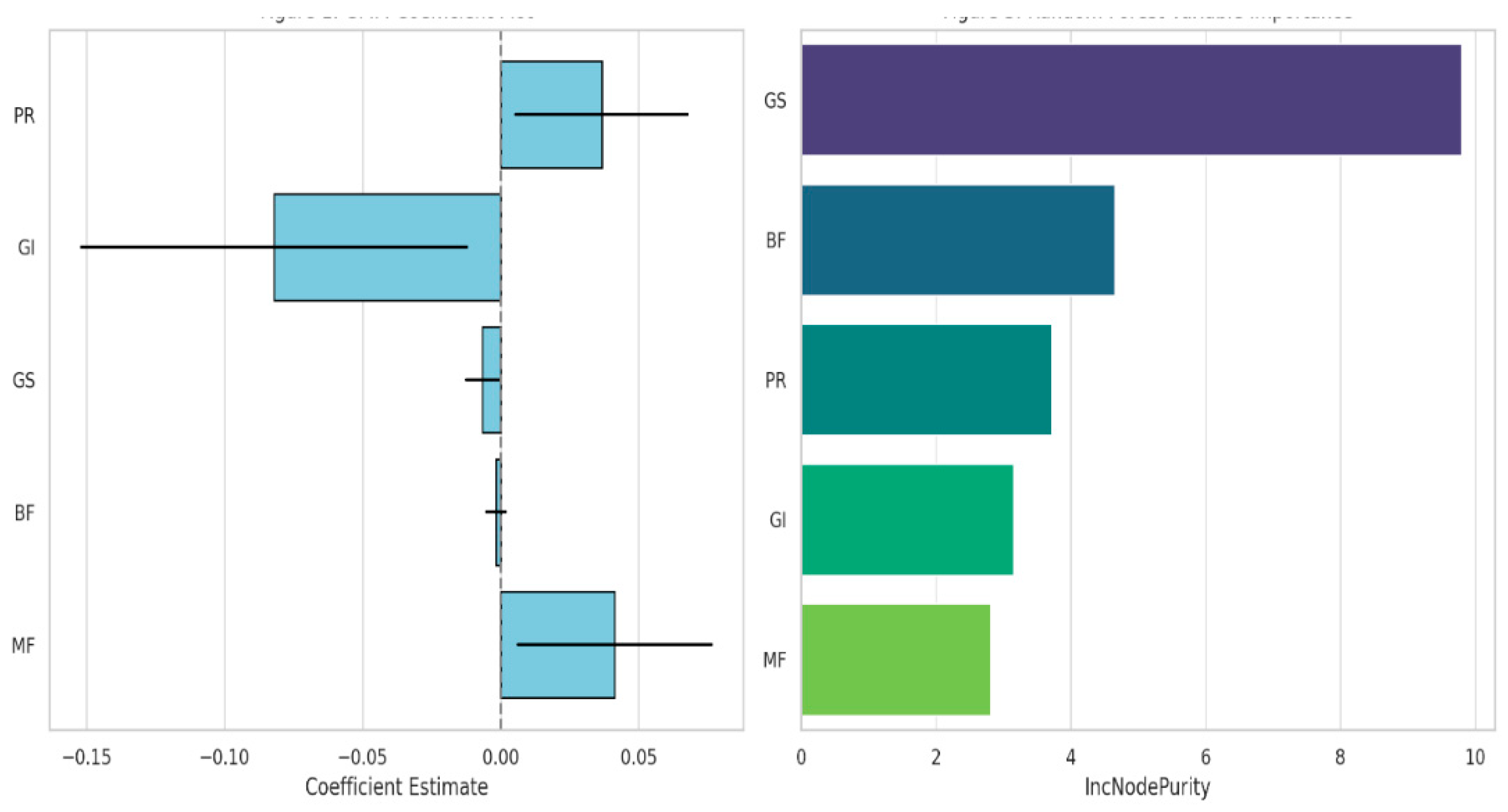
Figure 2.
Impulse Response Function (Bayesian VAR).
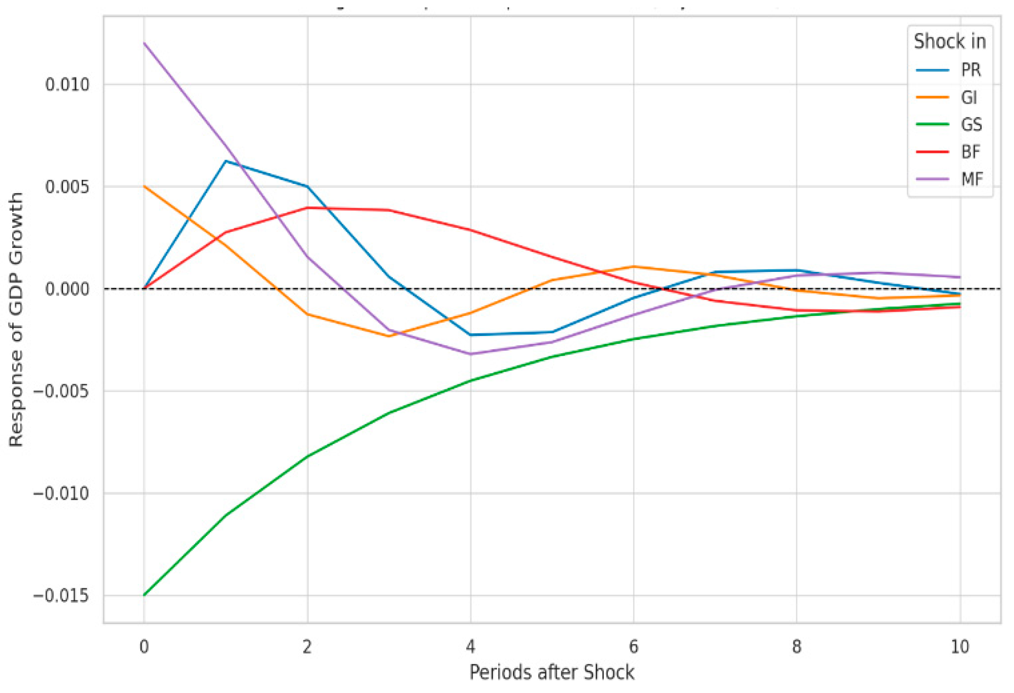
Table 3.
Descriptive Statistics (2013–2023).
| Variable | Mean | Std. Dev. | Min | Max |
| GDP Growth (%) | 2.45 | 1.26 | -0.8 | 5.8 |
| Property Rights (PR) | 61.8 | 9.6 | 43.5 | 79.1 |
| Government Integrity | 41.2 | 8.3 | 24.3 | 56.7 |
| Government Spending | 29.4 | 5.1 | 18.6 | 39.8 |
| Business Freedom (BF) | 66.3 | 11.2 | 39.2 | 84.7 |
| Monetary Freedom (MF) | 70.1 | 5.7 | 58.1 | 80.5 |
Table 4.
Correlation Matrix.
| Variable | GDP | PR | GI | GS | BF | MF |
| GDP | 1.00 | |||||
| PR | 0.31 | 1.00 | ||||
| GI | 0.12 | 0.22 | 1.00 | |||
| GS | -0.24 | -0.17 | -0.29 | 1.00 | ||
| BF | 0.19 | 0.33 | 0.11 | -0.13 | 1.00 | |
| MF | 0.28 | 0.25 | 0.14 | -0.09 | 0.18 | 1.00 |
Table 5.
Variance Inflation Factors (VIF).
| Variable | VIF |
| Property Rights (PR) | 1.83 |
| Government Integrity | 1.62 |
| Government Spending | 1.47 |
| Business Freedom (BF) | 1.91 |
| Monetary Freedom (MF) | 1.55 |
Table 6.
GMM Regression Results (Dependent Variable: GDP per capita growth).
| Variable | Coefficient | Std. Error | z-value | p-value | Sig. |
| GDP(-1) | 0.9384 | 0.0248 | 37.85 | <0.0001 | *** |
| Constant | -0.7116 | 0.4304 | -1.653 | 0.0983 | * |
| Property Rights (PR) | 0.0367 | 0.0159 | 2.312 | 0.0208 | ** |
| Government Integrity (GI) | -0.0820 | 0.0354 | -2.315 | 0.0206 | ** |
| Government Spending (GS) | -0.0066 | 0.0031 | -2.155 | 0.0312 | ** |
| Business Freedom (BF) | -0.0017 | 0.0018 | -0.949 | 0.3428 | NS |
| Monetary Freedom (MF) | 0.0413 | 0.0180 | 2.289 | 0.0221 | ** |
Table 7.
Bayesian VAR – GDP Growth Equation.
| Variable | Coefficient | Std. Error |
| GDP Growth (-1) | 0.7169 | 0.0373 |
| GDP Growth (-2) | 0.2811 | 0.0371 |
| Constant | 0.3694 | 0.1506 |
| Government Integrity (GI) | 0.0028 | 0.0125 |
| Government Spending (GS) | 0.0006 | 0.0012 |
| Monetary Freedom (MF) | -0.0016 | 0.0062 |
| Property Rights (PR) | -0.0015 | 0.0055 |
| Business Freedom (BF) | 0.0001 | 0.0006 |
Table 8.
(a) Model Summary – Random Forest. (b) Variable Importance – IncNodePurity.
| (a) | |
| Metric | Value |
| Type of Model | Regression |
| No. of Trees | 500 |
| Variables per Split | 3 |
| R-squared | 0.904 |
| RMSE | 0.408 |
| Mean Squared Error | 0.144 |
| (b) | |
| Variable | IncNodePurity |
| Government Spending (GS) | 9.80 |
| Business Freedom (BF) | 4.65 |
| Property Rights (PR) | 3.72 |
| Government Integrity (GI) | 3.15 |
| Monetary Freedom (MF) | 2.81 |
Table 9.
Summary of Empirical Findings.
| Method | PR | GI | GS | BF | MF | Notes |
| GMM | + ** | − ** | − ** | NS | + ** | High explanatory power; significant effects observed |
| Bayesian VAR | NS | NS | NS | NS | NS | Strong autoregressive structure; muted direct EF effects |
| Random Forest | Top 3 | Mid | Top | Top 2 | Lowest |
Disclaimer/Publisher’s Note: The statements, opinions and data contained in all publications are solely those of the individual author(s) and contributor(s) and not of MDPI and/or the editor(s). MDPI and/or the editor(s) disclaim responsibility for any injury to people or property resulting from any ideas, methods, instructions or products referred to in the content. |
© 2025 by the authors. Licensee MDPI, Basel, Switzerland. This article is an open access article distributed under the terms and conditions of the Creative Commons Attribution (CC BY) license (http://creativecommons.org/licenses/by/4.0/).
Copyright: This open access article is published under a Creative Commons CC BY 4.0 license, which permit the free download, distribution, and reuse, provided that the author and preprint are cited in any reuse.


