
Submitted:
01 July 2025
Posted:
03 July 2025
You are already at the latest version
Abstract
This study presents a comparative analysis of bearing and rotating component fault classification based on different time–frequency representations using ViT-base model. Four different time–frequency transformation techniques—Short-Time Fourier Transform (STFT), Continuous Wavelet Transform (CWT), Hilbert-Huang Transform (HHT), and Wigner-Ville Distribution (WVD)—were applied to convert the signals into 2D images. A pre-trained ViT-Base architecture was fine-tuned on the resulting images for classification tasks. The model was evaluated on two separate scenarios: (i) eight-class rotating component fault classification and (ii) four-class bearing fault classification. Importantly, in each task, the samples were collected under varying conditions of the other component (i.e., different rotating conditions in bearing classification and vice versa). This design allowed for an independent assessment of the model’s ability to generalize across fault domains. The experimental results demonstrate that the ViT-based approach achieves high classification performance across various time–frequency representations, highlighting its potential for mechanical fault diagnosis in rotating machinery. Notably, the model achieved higher accuracy in bearing fault classification compared to rotating component faults, suggesting a higher sensitivity to bearing-related anomalies.
Keywords:
bearing fault classification
; rotating component fault classification
; short-time fourier transform
; continuous wavelet transform
; hilbert-huang transform
; wigner-ville distribution
; vision transformer
1. Introduction
Rotating machinery plays a vital role in many industrial applications, from manufacturing systems to power generation facilities. Among their core components, bearings and rotating components are susceptible to faults due to prolonged operation and varying load conditions. Such faults can lead to reduced system performance, unexpected downtime, and high maintenance costs, making early and reliable fault detection critically important.
One of the most widely used approaches for this purpose is vibration-based condition monitoring. Vibration signals carry rich information about the operating condition of machinery and can be analyzed in different domains: the time domain, which reflects the raw waveform; the frequency domain, which reveals spectral content; and the time–frequency domain, which captures how frequency components evolve over time. In the literature, these representations have been utilized in various studies, each showing varying levels of effectiveness depending on the type of fault being detected.
In time–frequency-based studies, spectrograms obtained through STFT [1,2,3,4,5,6,7] and scalograms derived from CWT [8,9,10,11,12,13] are commonly used. Additionally, alternative methods such as the HHT [14,15,16] and WVD [17,18,19] have also been employed in some works.
In recent years, convolutional neural network (CNN)-based models have been widely adopted in fault classification tasks using these representations. On the other hand, although Transformer-based architectures have achieved remarkable success in fields such as natural language processing and image classification, their application to bearing and rotating component fault diagnosis has so far remained limited.
In this study, the classification of bearing and rotating component faults was comparatively evaluated using various time–frequency representations. The raw signals were transformed into visual formats using four different time–frequency transformation techniques: STFT, CWT, HHT and WVD. These images were then fed into a ViT, a cutting-edge deep learning architecture originally developed for image classification tasks. The ViT-Base model was specifically employed, as it has not yet been widely explored in the context of bearing and rotating component fault classification. The goal was to assess the capability of ViT-Base in this domain and to compare its performance against conventional CNN-based models that are more commonly used in the existing literature.
The model’s performance was evaluated through two separate classification tasks: a four-class bearing fault classification (H, B, IR, OR), and an eight-class rotating component fault classification (H, L, M1, M2, M3, U1, U2, U3). In the bearing fault task, each sample corresponds to a specific bearing condition, but the data were collected under various rotating component states (e.g., L, U1, etc.). Similarly, in the rotating component fault task, each sample represents a specific rotating fault type, while being recorded under different bearing fault conditions (e.g., B, IR, etc.). This experimental design enables the assessment of the model’s ability to classify one type of fault independently of the other, and allows for a comparative analysis of classification performance across different time–frequency representations using ViT.
2. Time-Frequency Representation
A signal is typically analyzed within two fundamental domains: the time domain and the frequency domain. In the time domain, the focus is on examining how the amplitude of the signal varies over time, providing insights into the signal’s temporal behavior. However, this approach is insufficient for identifying the specific frequency components present within the signal. Conversely, the frequency domain analysis, commonly performed using the Fourier Transform (FT), reveals the complete spectral content of the signal, allowing for a detailed assessment of its frequency characteristics. Despite its effectiveness in uncovering frequency information, Fourier analysis inherently loses the temporal localization of these components, making it challenging to determine when certain frequencies occur within the signal:
where X(f) represents the fourier transform of the signal, indicating its frequency spectrum, f denotes the frequency variable in Hz, t represents time, j is the imaginary unit, dt indicates integration over the entire time domain from -∞ to +∞.
This transformation reveals the frequency components present in the signal over its entire time span. However, while it provides a comprehensive view of the signal’s spectral content, it lacks the ability to capture how these frequency characteristics evolve over time. This limitation makes it insufficient for analyzing non-stationary signals where frequency components change dynamically.
To address this limitation, the concept of time-frequency representation was introduced, aiming to analyze signals in both the time and frequency domains simultaneously. This idea was initially explored in the 1940s through the pioneering work of Gabor [20] and Ville [21]. Gabor approached the time-frequency plane by interpreting signals as composed of discrete units of information, while Ville focused on capturing the energy distribution within this domain. Their contributions laid the foundation for modern time-frequency analysis techniques, which are now essential in understanding complex, time-varying signals.
2.1. Spectrogram
In time series analysis, it is often essential to examine both the time and frequency characteristics of a signal simultaneously. This is particularly important in fields such as vibration analysis, audio processing, biomedical signal interpretation, and fault detection. One of the most widely used tools for such analysis is the spectrogram, which visually represents how the frequency content of a signal evolves over time.
Spectrograms are generated using the Short-Time Fourier Transform (STFT), which analyzes non-stationary signals by dividing them into short, overlapping time segments and applying the Fourier Transform to each segment. This method provides a time–frequency representation of the signal. Mathematically, the STFT is defined as:
where X(t,f) is the STFT of the signal, representing its time-frequency representation, x(τ) is the original time-domain signal to be analyzed, w(τ-t) is the window function that localizes the signal in the time domain, centered around time t. t denotes the time shift parameter, indicating the current position of the window and τ is the integration variable corresponding to time.
One of the key parameters in STFT is the window length, which determines the trade-off between time and frequency resolution. A shorter window offers better time resolution, making it ideal for detecting sudden changes or transient events. However, it reduces frequency resolution, making it difficult to distinguish closely spaced frequencies. Conversely, a longer window improves frequency resolution but limits the ability to detect rapid changes. This trade-off reflects the uncertainty principle in time–frequency analysis.
In addition to window length, the overlap between adjacent windows also affect the quality of the spectrogram. Higher overlap helps maintain continuity and reduces artifacts. Empirical studies suggest practical guidelines for optimizing STFT parameters in vibration signal analysis: setting the overlap to approximately 15/16 of the window length, using window lengths of at least 64 samples, keeping the window length under one-fourth of the total signal length, and selecting lengths as powers of two (e.g., 64, 128, 256) for computational efficiency [22].
A comprehensive search was conducted in the Web of Science (WOS) database using the following keyword combination: (“Bearing” OR “bearings” OR “Rotating Machinery”) AND (“Machine Learning” OR “Deep Learning” OR “Neural Network”) AND (“Fault Diagnosis” OR “Fault Detection” OR “Fault Classification”) AND (“Spectrogram” OR “Short-time Fourier Transform” OR “STFT”), with the aim of examining how the STFT technique has been applied to motor fault diagnosis in the existing literature. The search was limited to the title, abstract, and keywords of the publications. As a result, 84 journal articles and 16 conference proceedings were identified. Some of these studies are presented in Table 1.
In these studies, datasets such as the Case Western Reserve University (CWRU) [23], Machine Failure Prevention Technology (MFPT) [24] and Paderborn [25] datasets have been utilized. As input data, vibration signals [1,2,3,5,6], acoustic emission [4], and sound data [7] were commonly preferred. Various deep learning models have been employed, including CNN [1,2,6], Deep Residual Neural Networks (DRNN) [3], Large Memory Storage and Retrieval (LAMSTAR) Neural Networks [4], Categorical Generative Adversarial Networks (CatGAN) [5], and Stacked Sparse Autoencoders [7]. These studies collectively highlight the diversity of data sources and model architectures used in spectrogram-based fault classification.
2.2. Scalogram
While STFT provides a fixed-resolution time–frequency analysis, it faces limitations in balancing time and frequency resolution due to its constant window size. In contrast, the CWT offers a flexible, multi-resolution approach by adapting the analysis window size according to frequency. This makes CWT particularly well-suited for analyzing non-stationary signals that contain both transient and long-duration components.
CWT operates by convolving the signal with scaled and shifted versions of a selected mother wavelet function. The CWT of a signal x(t) is defined as:
where a is the scale parameter controlling frequency content, b is the translation parameter controlling time localization, and ψ(t) is the mother wavelet. Smaller scales (low a) correspond to higher frequencies and offer finer time resolution, while larger scales (high a) capture lower frequencies with better frequency resolution.
The output of CWT is a complex-valued matrix of coefficients that describe the signal’s similarity to the wavelet at various scales and time points. The scalogram is obtained by plotting the squared magnitude of these coefficients in a two-dimensional image, with time on the x-axis, scale on the y-axis, and color intensity representing amplitude. This representation reveals how energy is distributed in both time and frequency, capturing localized features and transients that are often not visible in time-only or frequency-only analyses.
A comprehensive search was conducted in the WOS database using the following keyword combination: (“Bearing” OR “bearings” OR “Rotating Machinery”) AND (“Machine Learning” OR “Deep Learning” OR “Neural Network”) AND (“Fault Diagnosis” OR “Fault Detection” OR “Fault Classification”) AND (“Scalogram” OR “Continuous Wavelet Transform” OR “CWT”), with the aim of examining how the CWT technique has been applied to motor fault diagnosis in the existing literature. The search was limited to the title, abstract, and keywords of the publications. As a result, 104 journal articles and 9 conference proceedings were identified. Some of these studies are presented in Table 2.
2.3. Hilbert Spectrum
The Hilbert-Huang Transform (HHT) is a time–frequency analysis method designed specifically for non-linear and non-stationary signals. It consists of two main stages: Empirical Mode Decomposition (EMD) and Hilbert Spectral Analysis (HSA).
In the first stage, the input signal is decomposed into a finite set of intrinsic mode functions (IMFs) using EMD. Each IMF is a simple oscillatory mode that satisfies specific mathematical criteria, allowing it to represent a single frequency component with well-behaved amplitude and frequency variations over time. Once the signal is decomposed into its IMFs, each component is subjected to the Hilbert Transform to obtain its instantaneous frequency and amplitude.
The Hilbert Transform of an IMF c(τ) is defined as:
where ĉ(t) is the Hilbert Transform of c(τ), and P⋅V⋅ denotes the Cauchy principal value. The analytic signal is then formed as:
Here, A(t) is the instantaneous amplitude and θ(t) is the instantaneous phase, from which the instantaneous frequency can be derived as:
By combining the instantaneous amplitudes and frequencies of all IMFs, the Hilbert Spectrum is constructed. It provides a detailed time–frequency–amplitude representation of the signal and is especially valuable for characterizing transient and non-linear behaviors.
A comprehensive search was conducted in the WOS database using the following keyword combination: (“Bearing” OR “bearings” OR “Rotating Machinery”) AND (“Machine Learning” OR “Deep Learning” OR “Neural Network”) AND (“Fault Diagnosis” OR “Fault Detection” OR “Fault Classification”) AND (“Hilbert Spectrum” OR “Hilbert-Huang Transform” OR “HHT”). The search was limited to the title, abstract, and keywords of the publications. As a result, 14 journal articles and 4 conference proceedings were identified. Some of these studies are presented in Table 3.
2.4. Wigner-Ville Spectrum
The Wigner-Ville Distribution (WVD) is a quadratic time–frequency representation that offers high resolution in both time and frequency domains. Unlike linear transforms, WVD is a member of the Cohen class of distributions and provides an energy-preserving representation of a signal’s instantaneous frequency content. It is particularly effective for analyzing non-stationary signals with rapid frequency variations or multi-component structures.
Mathematically, the Wigner-Ville Distribution of a signal x(t) is defined as:
Here, x*(t) denotes the complex conjugate of the signal x(t), t is time, f is frequency, and τ is the lag variable. The result is a real-valued function Wx(t,f) that describes the energy distribution of the signal over the time–frequency plane.
WVD has the ability to localize signal components with great precision, even in the presence of rapid frequency modulations. It directly reflects the signal’s instantaneous power, making it suitable for detailed signal characterization. However, because of its quadratic nature, WVD may also produce cross-terms when analyzing multi-component signals, which can complicate the interpretation of the resulting time–frequency distribution. These cross-terms are mathematical interference artifacts that arise due to the bilinear structure of the transform.
A comprehensive search was conducted in the WOS database using the following keyword combination: (“Bearing” OR “bearings” OR “Rotating Machinery”) AND (“Machine Learning” OR “Deep Learning” OR “Neural Network”) AND (“Fault Diagnosis” OR “Fault Detection” OR “Fault Classification”) AND (“Wigner-Ville Distribution” OR “WVD”). The search was limited to the title, abstract, and keywords of the publications. As a result, 5 journal articles were identified. Some of these studies are presented in Table 4.
3. Materials and Methods
3.1. Dataset
In this study, a multi-domain vibration dataset under compound machine fault scenarios was utilized [27]. This dataset provides a comprehensive collection of vibration signals obtained using a deep groove ball bearing (MOCHU 6204) under various fault conditions for fault diagnosis in rotating machinery. The dataset includes three different singular bearing faults, seven different singular rotating component faults, and 21 combined fault scenarios [28]. Data was collected at different rotational speeds of 600, 800, 1000, 1200, 1400, and 1600 RPM, with sampling rates of 8 kHz and 16 kHz, and for different bearing types. Each vibration signal was recorded for 160 seconds at an 8 kHz sampling rate and 80 seconds at a 16 kHz sampling rate, with each recording containing a total of 1,280,000 samples. The dataset is structured hierarchically based on sampling rate and rotational speed, with 32 data files available for each speed category.
The dataset defines various conditions that allow for the examination of rotating components and bearings under different fault scenarios. In terms of rotating component status, the system categorizes components as healthy (H), misaligned (M, severity levels 1-3), unbalanced (U, severity levels 1-3), and mechanically loose (L). Similarly, bearing conditions are classified according to different fault scenarios, with healthy bearings (H), bearings with ball faults (B), bearings with inner ring faults (IR), and bearings with outer ring faults (OR).
In this study, data collected at a 16 kHz sampling frequency and 1000 RPM rotational speed was utilized. Rotating component and bearing faults were identified separately. For the classification of rotating component faults, all data files containing the same type of rotating component fault were combined. This dataset includes both different healthy bearing data and data with various bearing faults. In other words, while detecting rotating component faults, the bearing condition in the dataset varies; some data contain healthy bearings, while others include ball faults, inner ring faults, or outer ring faults. Similarly, for the classification of bearing faults, all data files containing the same type of bearing fault were combined. In this process, the dataset includes records with different rotating component faults or healthy rotating components. That is, while identifying bearing faults, the condition of rotating components varies, with some data containing entirely healthy rotating components, while others include different faults such as misalignment, unbalance, or mechanical looseness.
Subsequently, various transformation algorithms were applied to the dataset to obtain different time-frequency representations for feature extraction based on time-frequency analysis. First, STFT was employed to analyze the frequency components of signals within specific time intervals, generating Spectrogram images. Then, CWT was utilized to produce scalogram images, offering an adaptive frequency resolution. Additionally, the WVD transformation was applied to visualize the signal’s autocorrelation-based analysis, resulting in the Wigner-Ville Spectrum. Finally, the HHT was used to determine the instantaneous frequency components of the signals, producing the Hilbert Spectrum. The time-frequency images obtained through these transformations were used to train deep learning-based model for machine fault diagnosis and condition monitoring.
In the time-frequency analysis that was conducted using the Short-Time Fourier Transform (STFT), a sampling frequency of 16,000 Hz was utilized. The Hann window, which is provided as the default option in the scipy.signal.spectrogram function, was employed with a window length set to 256 samples. To maintain temporal continuity between successive frames, an overlap of 32 samples—equivalent to one-eighth of the window length—was applied. The length of the Fast Fourier Transform (FFT) was configured to match the window length, specifically 256 points, in order to achieve a compromise between computational efficiency and frequency resolution. The spectrograms that were generated through this process were subsequently log-scaled, and they were visualized using Gouraud shading, which was applied to enhance the smoothness and clarity of the time-frequency representation.
In the scalogram-based time-frequency analysis, the Continuous Wavelet Transform (CWT) was carried out using the Morlet wavelet, which is known for providing a favorable trade-off between time and frequency localization. Each segment of the signal was composed of 16,000 samples. A range of scales, corresponding to wavelet widths varying from 1 to 30, was employed in the analysis. This range of scales was selected to enable the effective extraction of both low-frequency and high-frequency components from the signal, thereby ensuring a comprehensive representation of its spectral content.
For the time-frequency analysis based on the Hilbert-Huang Transform (HHT), Empirical Mode Decomposition (EMD) was applied using the mask sift approach, with the decomposition limited to a maximum of five intrinsic mode functions (IMFs). Each input segment was composed of 16,000 data samples, thereby maintaining consistency with the analyses conducted using the STFT and CWT methods. After the decomposition process was completed, the Normalized Hilbert Transform was subsequently applied to each extracted IMF in order to derive instantaneous frequency and amplitude information. The resulting time-frequency representations were then constructed using 150 frequency bins that were logarithmically spaced across the range from 1 Hz to 8,000 Hz. This configuration was chosen to enable a detailed and comprehensive characterization of both low-frequency and high-frequency components present in the signal.
For the Wigner-Ville Distribution (WVD) analysis, each original signal segment consisting of 16,000 samples was divided into smaller subsegments of 2,000 samples in order to reduce the computational and memory demands typically associated with generating the full WVD matrix. If the WVD were to be computed over the entire segment, a matrix of size 16,000 × 16,000 — containing 256 million elements—would be required, which is considered impractical due to significant memory constraints. By employing subsegments of 2,000 samples, the matrix size was effectively reduced to 2,000 × 2,000, resulting in only 4 million elements and thereby allowing for more efficient and feasible computation. The time-frequency representations that were obtained through this method were subsequently normalized by scaling the absolute values to the [0, 1] range, ensuring consistency, comparability, and interpretability across different signal samples.
The obtained image samples are presented in Figure 1. Table 5 summarizes the number of image samples generated for each time-frequency representation method. For the STFT, CWT, and HHT representations, a total of 2,560 samples were created for each method, distributed as 1,792 for training, 384 for validation, and 384 for testing. In contrast, the WVD representation resulted in a significantly larger dataset, comprising 14,336 training, 3,072 validation, and 3,072 test samples, totaling 20,480. This discrepancy arises from the specific subsegmentation strategy applied to the original signal prior to WVD computation. Since WVD involves a quadratic time and memory complexity, requiring an N×N matrix for a signal of length N the original 16,000-sample segments were split into smaller 2,000-sample subsegments to prevent memory overflow. This adjustment was essential to ensure computational feasibility and to avoid exceeding hardware limitations during the generation of WVD-based time-frequency images.
3.2. Method
The overall structure of the ViT-based fault classification approach used in this study is illustrated in Figure 2. Vibration signals are first transformed into time–frequency representations using one of four methods: STFT, CWT, HHT or WVD. The resulting 2D image is resized to 224×224 pixels and fed into a ViT architecture. The input image is divided into non-overlapping patches of size 16×16 pixels, flattened, and linearly projected. Positional embeddings are then added, and the embedded patches are processed through transformer encoder blocks consisting of multi-head self-attention and feed-forward (MLP) layers. The output token is finally passed to a classification head (MLP Head) to predict the corresponding fault class.
A pre-trained ViT-Base model was employed, and a transfer learning strategy was applied. To reduce computational cost and training time, all layers were frozen except for the final classification head, which was fine-tuned on the target dataset. For visualization clarity, only 9 patches are shown in the figure; in practice, the input image is divided into 14×14 = 196 patches.
To evaluate the model’s performance, two independent classification tasks were conducted. In the first task, , an eight-class rotating component fault classification (H, L, M1, M2, M3, U1, U2, U3) was performed; in the second a four-class bearing fault classification (H, B, IR, OR) was carried out. In both tasks, the samples were intentionally constructed to include varying conditions of the other component. That is, bearing fault samples were collected under different rotating component states, while rotating component fault samples were collected under varying bearing conditions. This structure ensures that the model learns to identify fault types independently of variations in other mechanical components, allowing for a more realistic and robust evaluation.
4. Experimental Results
ViT-based architecture was utilized in this study for image-based fault classification. The pre-trained ‘vit-base-patch16-224’ model from the Hugging Face library was employed, with only the final classification layer fine-tuned. The optimizer used was Adam with a learning rate of 0.001, and cross-entropy was selected as the loss function. The batch size was set to 32. An ‘EarlyStopping’ mechanism with a patience of 5 epochs was implemented to prevent overfitting. The dataset was split in a balanced manner across classes, with 70% of the data used for training, 15% for validation, and 15% for testing.
4.1. STFT Results
Performance metrics on the test dataset using spectrograms are presented in Table 6. The table reports precision, recall, F1-score and accuracy values for two main fault types: rotating component faults and bearing faults. For rotating component faults, all metrics are reported as 88%, whereas for bearing faults, these metrics reach a notably high level of 99%. This indicates that the spectrogram-based approach yields more successful results in detecting bearing faults.
Table 7 displays the confusion matrix for the classification of rotating component faults. A closer examination reveals that different severity levels of the same fault type (e.g., M1, M2, M3 or U1, U2, U3) are more frequently confused with one another. For instance, 6 instances of the U1 class were misclassified as U2, and 4 as U3. Similarly, 4 instances from the U3 class were predicted as U2. This suggests that the model struggles to distinguish between different severity levels within the same fault type. In contrast, different fault types (e.g., H and L, or the M-series and U-series faults) are generally well-classified, indicating a clearer separation between these categories in the feature space.
Table 8 presents the confusion matrix for the classification of bearing faults. As seen in the table, all classes exhibit a high number of correctly classified instances. This demonstrates that bearing faults present more distinct characteristics compared to other classes, allowing the model to differentiate them more easily.
4.2. CWT Results
In Table 9, the performance metrics on the test dataset obtained using scalogram are presented. Precision, recall, F1-score, and accuracy values are reported for two main fault types: rotating component faults and bearing faults. For rotating component faults, the metrics are around 86–87%, whereas for bearing faults, all values reach 97%. These results indicate that the scalogram-based method is particularly effective in detecting bearing faults, while its performance on rotating component faults is comparatively lower.
Table 10 presents the confusion matrix generated by the scalogram-based model for the classification of rotating component faults. Similar to previous findings, different severity levels of the same fault type tend to be misclassified among each other. For instance, 6 samples from class M2 were misclassified as M3, and 4 as M1. Likewise, 4 samples from class U1 were predicted as U2, and 6 as U3. In the case of class U3, there is a notable confusion with U2, with 10 samples incorrectly classified. These results highlight the model’s ongoing difficulty in distinguishing between varying severity levels within the same fault type. In contrast, clearly distinct fault types such as H and L were classified with high accuracy.
Table 11 displays the confusion matrix for bearing fault classification using the scalogram-based approach. Although 3 samples of class B were misclassified as H, and 7 samples of H were classified as B, overall, the scalogram-based method still achieves high accuracy in detecting bearing faults.
4.3. HHT Results
In Table 12, the performance metrics on the test dataset obtained using the Hilbert spectrum are presented. For rotating component faults, the accuracy, precision, recall, and F1-score remain within the range of 69–71%, while for bearing faults, these metrics reach 90%. This indicates that, similar to previous methods, the HHT-based approach yields higher performance in bearing fault detection but remains limited in detecting rotating component faults.
Table 13 presents the confusion matrix for the classification of rotating component faults using the HHT-based model. The matrix reveals a high level of confusion between classes. In particular, for classes M2 and U1, only 26 out of 48 samples were correctly classified, highlighting the model’s difficulty in distinguishing between these fault types.
Table 14 shows the confusion matrix for bearing fault classification. In this case, the model exhibited its poorest performance when classifying samples from class H. Specifically, 12 samples from B were classified as H, 2 as IR, and 3 as OR.
4.4. WVD Results
Table 15 presents the performance metrics of the WVD-based approach in the classification of rotating component and bearing faults. The results indicate that the model achieves a remarkably high performance in classifying bearing faults, with 99% accuracy, precision, recall, and F1-score. This demonstrates the model’s effectiveness in correctly identifying positive samples of bearing faults while minimizing false positives. In contrast, the performance metrics for rotating component faults remain at 84%, suggesting that the model is relatively less successful in distinguishing between these fault types.
As shown in Table 16 the confusion matrix for rotating component faults reveals a concentration of misclassifications within specific classes. Notably, the M2 class has the lowest number of correctly classified samples (257), indicating challenges in accurately identifying this fault type. The highest classification performance is observed for class L, while a significant number of misclassifications are associated with the H class. Specifically, 108 samples that do not belong to class H were incorrectly classified as H, indicating that the model tends to overpredict the healthy condition.
Table 17 provides the confusion matrix for bearing faults and shows minimal classification errors among the classes. For instance, only one sample was misclassified in the IR class, and all samples in the OR class were correctly identified. These findings suggest that bearing faults exhibit more distinctive features, allowing the WVD-based method to perform highly effectively in this context.
5. Discussion
Table 18 presents a comparative evaluation of classification accuracies achieved by different deep learning models (ViT-base, ResNet101, and DenseNet121) using four time-frequency representations: Spectrogram, Scalogram, HHT and WVD. The analysis considers two fault types separately, namely rotating component faults and bearing faults, to comprehensively assess the discriminative capability of each representation-model pair.
When bearing fault classification is considered, WVD demonstrates a consistently high level of accuracy across all models, achieving 99% in every case, highlighting its superior ability to capture the characteristic patterns associated with bearing anomalies. This suggests that WVD effectively preserves time-frequency information, enabling the models to generalize well to different fault conditions in bearing systems.
In the classification of rotating component faults, the overall performance is noticeably lower than in the bearing fault scenario, regardless of the representation or model used. WVD generally provides strong performance for this fault type. However, it does not yield the highest accuracy across all models. For the ResNet101 and DenseNet121 architectures, WVD achieves the best results with accuracies of 90% and 86%, respectively. In contrast, for the ViT-base model, the spectrogram representation performs better, reaching an accuracy of 88%, while WVD achieves 84%. This indicates that although WVD is highly effective for convolutional neural networks, its compatibility with transformer-based architectures may be relatively limited in certain contexts.
Scalogram representations have yielded stable and competitive results across both fault categories and model architectures. In the classification of rotating component faults, scalogram achieves 86% accuracy with the ViT-base model, outperforming WVD in this specific case. For ResNet101 and DenseNet121, the accuracies are 85% in both, which are relatively close to those achieved using WVD. When bearing faults are considered, scalogram again performs consistently, achieving 97% with ViT-base, 96% with ResNet101, and 95% with DenseNet121. Although slightly lower than the top-performing WVD and spectrogram representations, these values still reflect a high level of classification performance. These results indicate that scalogram representations provide sufficient discriminative features and exhibit compatibility with different deep learning models, making them a reliable choice for vibration-based fault diagnosis tasks.
Interestingly, HHT appears to be the least effective representation for rotating component faults across all models. This could be attributed to the empirical mode decomposition (EMD) process used in HHT, which may not be sufficiently robust in capturing transient and modulated features in the presence of noise or complex signal interactions. Consequently, models trained on HHT representations tend to underperform, especially for rotating component faults.
Another important observation concerns the performance variation among models. While ViT-base performs competitively, it exhibits noticeable sensitivity to the representation type, as seen in the dramatic drop in accuracy with HHT. On the other hand, convolutional models such as ResNet101 and DenseNet121 demonstrate relatively more stable performance across different representations.
In a related study [29] utilizing the MFPT dataset, which involves the classification of H, IR, and OR conditions, scalogram representations achieved the highest classification accuracy of 99.9%, followed by HHT with 95.5% and spectrogram with 91.7%. Similarly, in the CWRU dataset comprising H, BF, IR, and OR classes, both spectrogram and scalogram achieved 99.5% accuracy, while HHT reached 97.6%. These results suggest that scalogram representations can deliver highly accurate fault diagnosis performance across various datasets.
In comparison, the results obtained in the present study using the same time-frequency representations demonstrate comparable, and in some cases even superior, classification performance. Specifically, in the classification of bearing faults using our custom dataset, scalogram achieved up to 97% accuracy with ViT-base, while spectrogram and WVD reached 99%. HHT, on the other hand, yielded slightly lower results, ranging from 90% to 94% depending on the model used. These findings confirm the robustness of spectrogram and scalogram representations, as highlighted in the previous study, while also emphasizing the strong performance of the WVD as an alternative representation capable of delivering top-tier accuracy levels.
One limitation of this study is that the data used were collected at a sampling frequency of 16 kHz and a rotational speed of 1000 RPM. Although the dataset itself includes a variety of operating conditions, only a specific subset was utilized in this work. This choice allowed for a consistent comparative analysis of the time–frequency representations under controlled conditions, but it also restricts the ability to directly assess the model’s performance under different speeds and sampling rates. In future studies, utilizing a broader portion of the dataset would enable a more comprehensive evaluation of the method’s generalizability across varying operating conditions.
6. Conclusion
This study presented a comprehensive comparison of four time–frequency transformation techniques, STFT (spectrogram), CWT (scalogram), HHT, and WVD, for the purpose of classifying faults in rotating and bearing components using a ViT-base architecture. By converting vibration signals into two-dimensional time–frequency representations, and fine-tuning a pre-trained ViT-base model on these images, the research explored the model’s effectiveness in two distinct diagnostic scenarios: rotating component fault classification and bearing fault classification. A key aspect of the experimental design was the introduction of cross-condition variability, where the non-target component was subjected to different fault states, thereby providing a more realistic and challenging evaluation of the model’s generalization ability.
The results indicate that the ViT-base model can successfully classify mechanical faults with high accuracy across different time–frequency representations, with particularly strong performance in the bearing fault classification task. Among the tested representations, spectrogram, scalogram, and WVD consistently delivered high accuracies, while HHT yielded comparatively lower results in both fault types. WVD, in particular, emerged as a promising representation, achieving top-tier results in several configurations and offering an effective alternative to more conventional approaches. Additionally, the study demonstrates that bearing faults are more readily detected than rotating component faults, likely due to their more distinctive signal characteristics. Overall, the findings suggest that ViT-based architectures, when combined with appropriate time–frequency representations, offer a powerful and flexible framework for fault diagnosis in rotating machinery.
Author Contributions
Conceptualization, A.O., M.E. and M.Z.; methodology, A.O., M.Z. and M.M.; software, N.Y. and M.E.; validation, A.O., M.Z. and M.M.; formal analysis, N.Y., M.E.; investigation, N.Y. and M.E.; writing—review and editing, N.Y., M.E., M.Z. and M.M.; visualization, N.Y. and M.E.; supervision, A.O., M.Z. and M.M. All authors have read and agreed to the published version of the manuscript.
Funding
This research received no external funding.
Data Availability Statement
The data used in this study are available online: Multi-domain vibration dataset with various bearing types under compound machine fault scenarios: subset 1 (deep groove ball bearing).
Acknowledgments
The authors would like to thank the Research and Development Sector at the Technical University of Sofia for the financial support.
Conflicts of Interest
The authors declare no conflicts of interest.
References
- Zhang, Q.; Deng, L. An Intelligent Fault Diagnosis Method of Rolling Bearings Based on Short-Time Fourier Transform and Convolutional Neural Network, J. Fail. Anal. Prev., 2023, 23(2), pp. 795-811. [CrossRef]
- Zhong, D.; Guo, W.; He, D. An Intelligent Fault Diagnosis Method based on STFT and Convolutional Neural Network for Bearings Under Variable Working Conditions, in 2019 Prognostics and System Health Management Conference (PHM-Qingdao), 2019, pp. 1-6. [CrossRef]
- Peng, B.; Xia, H.; Lv, X.; Annor-Nyarko, M.; Zhu, S.; Liu, Y.; Zhang, J. An intelligent fault diagnosis method for rotating machinery based on data fusion and deep residual neural network. Applied Intelligence, 2022, 52(3), pp. 3051-3065. [CrossRef]
- He, M.; He, D. Deep learning based approach for bearing fault diagnosis. IEEE Transactions on Industry Applications, 2017, 53(3), pp. 3057-3065. [CrossRef]
- Tao, H.; Wang, P.; Chen, Y.; Stojanovic, V.; Yang, H. An unsupervised fault diagnosis method for rolling bearing using STFT and generative neural networks. Journal of the Franklin Institute, 2020, 357(11), pp. 7286-7307, 2020. [CrossRef]
- Zhang, Y.; Xing, K.; Bai, R.; Sun, D.; Meng, Z. An enhanced convolutional neural network for bearing fault diagnosis based on time–frequency image. Measurement, 2020, 157, 107667. [Google Scholar] [CrossRef]
- Liu, H.; Li, L.; Ma, J. Rolling bearing fault diagnosis based on STFT-deep learning and sound signals. Shock and Vibration, 2016(1), 6127479. [CrossRef]
- Cheng, Y.; Lin, M.; Wu, J.; Zhu, H.; Shao, X. Intelligent fault diagnosis of rotating machinery based on continuous wavelet transform-local binary convolutional neural network. Knowledge-Based Systems, 2021, 216, 106796. [Google Scholar] [CrossRef]
- Xu, Y.; Li, Z.; Wang, S.; Li, W.; Sarkodie-Gyan, T.; Feng, S. A hybrid deep-learning model for fault diagnosis of rolling bearings. Measurement, 2021, 169, 108502. [Google Scholar] [CrossRef]
- Mian, T.; Choudhary, A.; Fatima, S. Vibration and infrared thermography based multiple fault diagnosis of bearing using deep learning. Nondestructive Testing and Evaluation, 2023, 38(2), 275-296. [CrossRef]
- Zhao, H.; Liu, J.; Chen, H.; Chen, J.; Li, Y.; Xu, J.; Deng, W. Intelligent diagnosis using continuous wavelet transform and gauss convolutional deep belief network. IEEE Transactions on Reliability, 2022, 72(2), 692-702. [CrossRef]
- Ahsan, M.; Hassan, M.W.; Rodriguez, J.; Abdelrahem, M. Enhanced Fault Diagnosis in Rotating Machinery Using a Hybrid CWT-LeNet-5-LSTM Model: Performance Across Various Load Conditions. IEEE Access, 2024. [CrossRef]
- Yu, S.; Li, Z.; Gu, J.; Wang, R.; Liu, X.; Li, L.; ... & Ren, Y. CWMS-GAN: A small-sample bearing fault diagnosis method based on continuous wavelet transform and multi-size kernel attention mechanism. PloS one, 2025, 20(4), e0319202. [CrossRef]
- Liu, H.; Wang, X.; Lu, C. Rolling Bearing Fault Diagnosis under Variable Conditions Using Hilbert-Huang Transform and Singular Value Decomposition. Mathematical Problems in Engineering, 2014(1), 765621. [CrossRef]
- Suthar, V.; Vakharia, V.; Patel, V.K.; Shah, M. Detection of compound faults in ball bearings using multiscale-SinGAN, heat transfer search optimization, and extreme learning machine. Machines, 2022, 11(1), 29. [CrossRef]
- Lin, S.L. Intelligent fault diagnosis and forecast of time-varying bearing based on deep learning VMD-DenseNet. Sensors, 2021, 21(22), 7467. [CrossRef]
- Wei, P.; Liu, M.; Wang, X. Few-shot bearing fault diagnosis using GAVMD–PWVD time–frequency image based on meta-transfer learning. Journal of the Brazilian Society of Mechanical Sciences and Engineering, 2023, 45(5), 277. [CrossRef]
- Hua, L.; Qiang, Y.; Gu, J.; Chen, L.; Zhang, X.; Zhu, H. Mechanical fault diagnosis using color image recognition of vibration spectrogram based on quaternion invariable moment. Mathematical problems in engineering, 2015(1), 702760. [CrossRef]
- Li, X.; Bi, F.; Zhang, L.; Lin, J.; Bi, X.; Yang, X. Rotating machinery faults detection method based on deep echo state network. Applied Soft Computing, 2022, 127, 109335. [CrossRef]
- Gabor, D. Theory of communication. Part 1: The analysis of information. Journal of the Institution of Electrical Engineers-part III: radio and communication engineering, 1946, 93(26), 429-441. [CrossRef]
- Ville, J. “Theorie et applications de la notion de signal analytique: Cables et Transmissions, 2A”, 1948.
- Jablonski, A.; Dziedziech, K. Intelligent spectrogram–A tool for analysis of complex non-stationary signals. Mechanical Systems and Signal Processing, 2022, 167, 108554. [Google Scholar] [CrossRef]
- “Apparatus & Procedures | Case School of Engineering”. Available online: https://engineering.case.edu/bearingdatacenter/apparatus-and-procedures (accessed on July 1, 2025).
- Bechhoefer, E. A quick introduction to bearing envelope analysis, MFPT Data. Available online: www.mfpt.org/fault-data-sets (accessed on July 1, 2025).
- Lessmeier, C.; Kimotho, J.K.; Zimmer, D.; Sextro, W. Condition monitoring of bearing damage in electromechanical drive systems by using motor current signals of electric motors: A benchmark data set for data-driven classification. In PHM society European conference, 2016, July, Vol. 3, No. 1. [CrossRef]
- Huang, H.; Baddour, N. Bearing vibration data collected under time-varying rotational speed conditions. Data in brief, 2018, 21, 1745–1749. [Google Scholar] [CrossRef] [PubMed]
- Lee, S.; Kim, T.; Kim, T. Multi-domain vibration dataset with various bearing types under compound machine fault scenarios: subset 1 (deep groove ball bearing), Mendeley data, 2024, V1. [CrossRef]
- Lee, S.; Kim, T.; Kim, T. Multi-domain vibration dataset with various bearing types under compound machine fault scenarios. Data in Brief, 2024, 57, 110940. [Google Scholar] [CrossRef] [PubMed]
- Verstraete, D.; Ferrada, A.; Droguett, E. L.; Meruane, V.; Modarres, M. Deep learning enabled fault diagnosis using time-frequency image analysis of rolling element bearings. Shock and Vibration, 2017(1), 5067651. [CrossRef]
Figure 1.
Samples of images in the dataset.
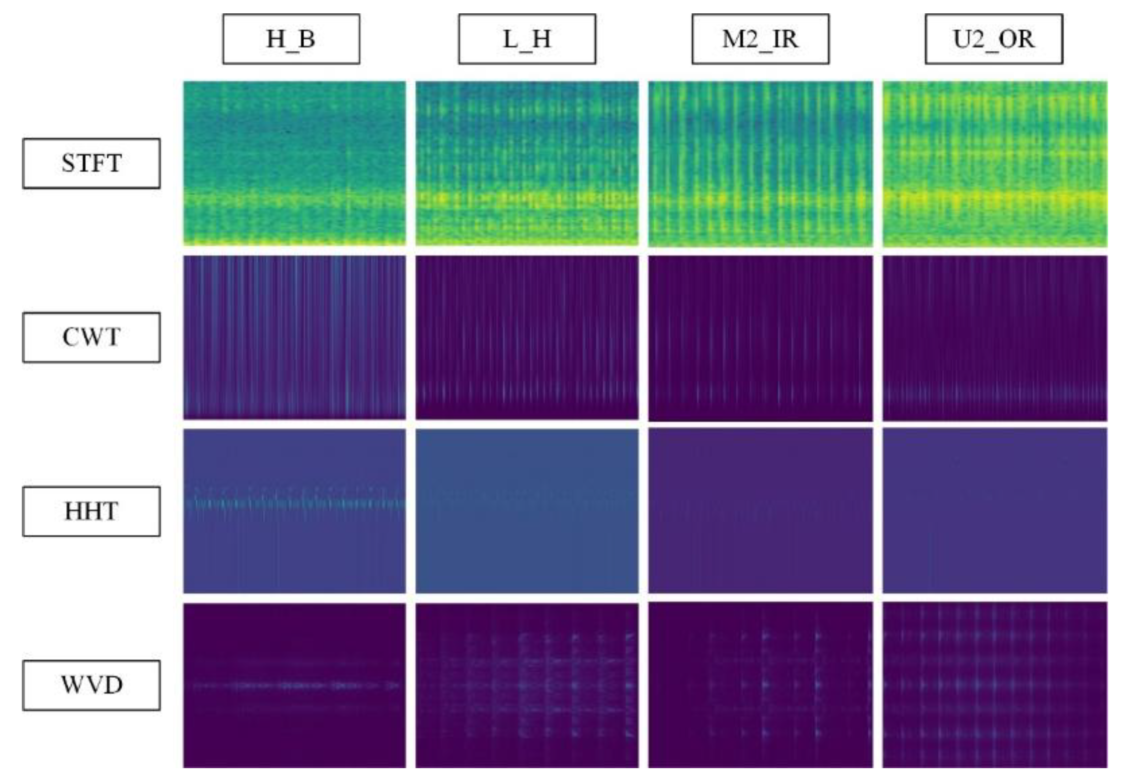
Figure 2.
Overall structure of the ViT-based fault classification approach.
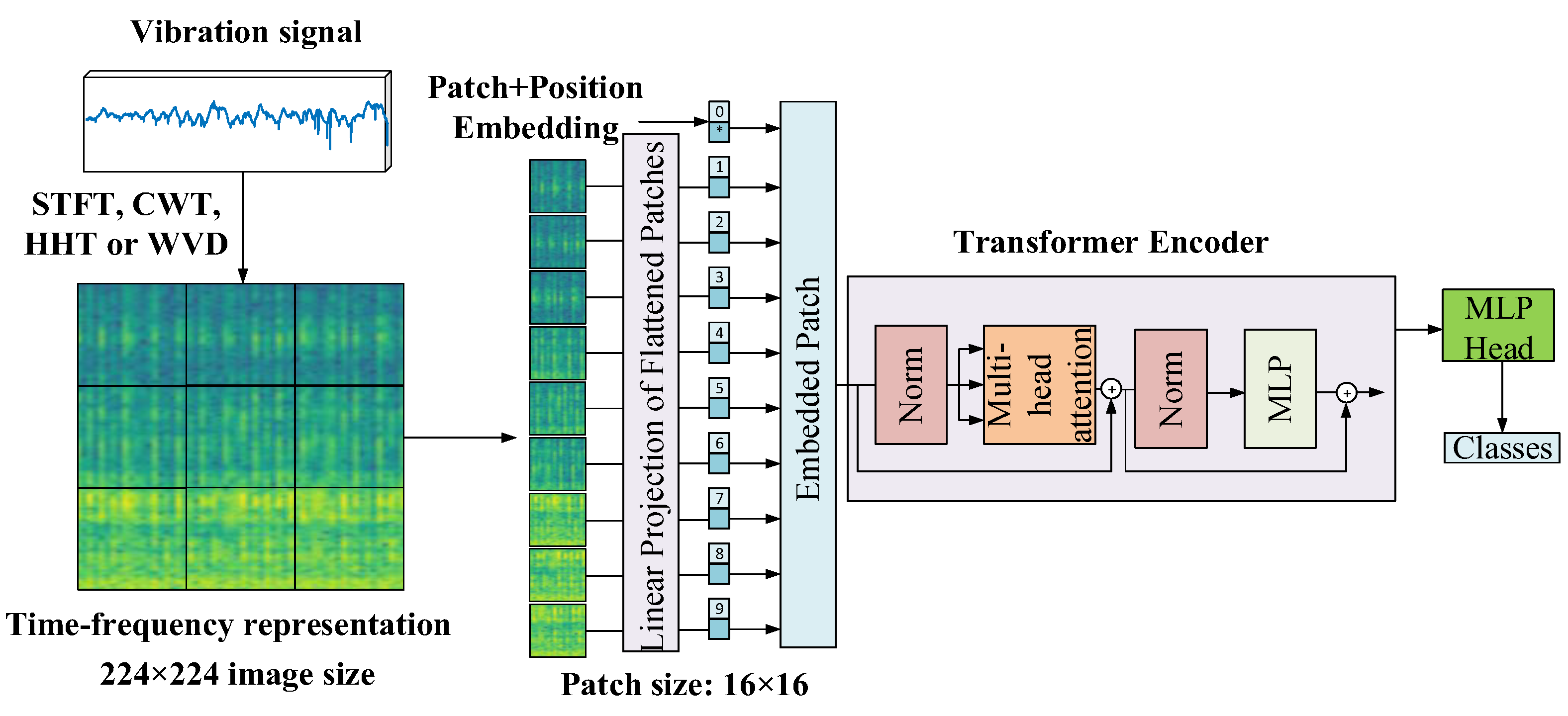

Table 1.
Summary of the studies utilizing spectrogram images for bearing fault classification.
| Ref. No | Dataset | Faults | Method | Results |
|---|---|---|---|---|
| [1] | CWRU [23] MFPT [24] |
CWRU: H (healthy), IR (inner race), OR (outer race), B (ball) MFPT: H, IR, OR |
CNN | CWRU=100% MFPT=99.96% |
| [2] | PADERBORN [25] | H, IR, OR | CNN | 97.48% |
| [3] | CWRU | H, IR, OR, B | DRNN | 99.86%, 99.91%, 99.88% |
| [4] | Private | H, IR, OR, B, C (cage) | LAMSTAR Neural Network | 96% to 100% |
| [5] | CWRU | H, three different damage diameter for B, IR and OR | CatGAN | 91.89% |
| [6] | CWRU Yanshan University dataset (YSU) |
CWRU: H, three different damage diameter for B, IR and OR YSU: H, IR, OR, B |
CNN | CWRU: 92.67±4.28% – 99.32±0.55% YSU: 97.81±0.71% |
| [7] | Private | H, IR, OR, B | Stacked sparse autoencoder | %96.29 |
Table 2.
Summary of the studies utilizing scalogram images for bearing fault classification.
| Ref. No | Dataset | Faults | Method | Results |
|---|---|---|---|---|
| [8] | MFPT | H, IR, OR | Local binary convolutional neural network (LBCNN) | 99.56±0.97 |
| [9] | CWRU XJTU-SY |
CWRU: H, IR, OR, B XJTU-SY: C, IR, OR |
CNN-gcForest | CWRU: 98.24% to 99.79% XJTU-SY: 99.8% |
| [10] | Private | H, IR, OR, B, LB (lack of lubrication), dual faults, multiple faults | CNN | 99.39% to 99.97% |
| [11] | CWRU | H, IR, OR, B | Gauss convolutional deep belief network (CDBN) | Four-classes:99.579% ten-classes: 99.028% |
| [12] | CWRU | H, IR, OR, B | LeNet-5-LSTM | 99.6% |
| [13] | CWRU MFPT |
CWRU: H, IR, OR, B MFPT: H, IR, OR |
CWMS-GAN | CWRU:99.83%, MFPT: 97.94% |
Table 3.
Summary of the studies utilizing hilbert-huang transform for bearing fault classification.
| Ref. No | Dataset | Faults | Method | Results |
|---|---|---|---|---|
| [14] | CWRU | H, IR, OR, B | Elman neural network | %100 |
| [15] | Private | H, three different fault severities for each of the B, IR, and OR | Extreme Learning Machine | 99.04% to 100% |
| [16] | University of Ottawa [26] | H, IR, OR, B, Combine | VMD-DenseNet | 92% |
Table 4.
Summary of the studies utilizing wigner-ville distribution for bearing fault classification.
Table 4.
Summary of the studies utilizing wigner-ville distribution for bearing fault classification.
| Ref. No | Dataset | Faults | Method | Results |
|---|---|---|---|---|
| [17] | CWRU | H, three different fault severities for each of the B, IR, and OR | Meta-transfer-learning and original relational network (MTLRN-AM) | 98% |
| [18] | CWRU | H, IR, OR, B | QIM-NWNN | 97.5% |
| [19] | CWRU | H, two different fault severities for each of the B, IR, and OR | Deep echo state network based on fixed convolution kernels FCK-DESN | 95.43% |
Table 5.
Sample numbers for each time-frequency representation.
| Time-frequency representation | Train | Validation | Test | Total |
|---|---|---|---|---|
| STFT | 1792 | 384 | 384 | 2560 |
| CWT | 1792 | 384 | 384 | 2560 |
| HHT | 1792 | 384 | 384 | 2560 |
| WVD | 14336 | 3072 | 3072 | 20480 |
Table 6.
Performance metrics on test dataset for spectrogram.
| Fault type | Precision (%) | Recall (%) | F1-score (%) | Accuracy (%) |
|---|---|---|---|---|
| Rotating component faults | 88 | 88 | 88 | 88 |
| Bearing faults | 99 | 99 | 99 | 99 |
Table 7.
Confusion matrix for rotating component faults classification and spectrogram.
| H | L | M1 | M2 | M3 | U1 | U2 | U3 | |
|---|---|---|---|---|---|---|---|---|
| H | 45 | 0 | 0 | 0 | 0 | 0 | 3 | 0 |
| L | 0 | 48 | 0 | 0 | 0 | 0 | 0 | 0 |
| M1 | 1 | 0 | 44 | 2 | 0 | 0 | 0 | 1 |
| M2 | 0 | 0 | 0 | 40 | 6 | 0 | 2 | 0 |
| M3 | 0 | 0 | 0 | 4 | 44 | 0 | 0 | 0 |
| U1 | 3 | 0 | 0 | 0 | 0 | 35 | 6 | 4 |
| U2 | 3 | 1 | 1 | 0 | 0 | 1 | 40 | 2 |
| U3 | 3 | 0 | 0 | 0 | 0 | 0 | 4 | 41 |
Table 8.
Confusion matrix for bearing faults classification and spectrogram.
| B | H | IR | OR | |
|---|---|---|---|---|
| B | 95 | 1 | 0 | 0 |
| H | 1 | 95 | 0 | 0 |
| IR | 0 | 0 | 96 | 0 |
| OR | 0 | 0 | 0 | 96 |
Table 9.
Performance metrics on test dataset for scalogram.
| Fault type | Precision (%) | Recall (%) | F1-score (%) | Accuracy (%) |
|---|---|---|---|---|
| Rotating component faults | 87 | 86 | 86 | 86 |
| Bearing faults | 97 | 97 | 97 | 97 |
Table 10.
Confusion matrix for rotating component faults classification and scalogram.
| H | L | M1 | M2 | M3 | U1 | U2 | U3 | |
|---|---|---|---|---|---|---|---|---|
| H | 48 | 0 | 0 | 0 | 0 | 0 | 0 | 0 |
| L | 0 | 48 | 0 | 0 | 0 | 0 | 0 | 0 |
| M1 | 0 | 0 | 46 | 1 | 0 | 0 | 1 | 0 |
| M2 | 0 | 0 | 4 | 35 | 6 | 0 | 1 | 2 |
| M3 | 0 | 0 | 0 | 4 | 42 | 0 | 0 | 2 |
| U1 | 0 | 0 | 0 | 0 | 1 | 37 | 4 | 6 |
| U2 | 0 | 2 | 0 | 1 | 1 | 1 | 41 | 2 |
| U3 | 0 | 1 | 0 | 0 | 0 | 2 | 10 | 35 |
Table 11.
Confusion matrix for bearing faults classification and scalogram.
| B | H | IR | OR | |
|---|---|---|---|---|
| B | 92 | 3 | 0 | 1 |
| H | 7 | 89 | 0 | 0 |
| IR | 0 | 0 | 96 | 0 |
| OR | 0 | 0 | 0 | 96 |
Table 12.
Performance metrics on test dataset for HHT.
| Fault type | Precision (%) | Recall (%) | F1-score (%) | Accuracy (%) |
|---|---|---|---|---|
| Rotating component faults | 71 | 69 | 69 | 69 |
| Bearing faults | 90 | 90 | 90 | 90 |
Table 13.
Confusion matrix for rotating component faults classification and HHT.
| H | L | M1 | M2 | M3 | U1 | U2 | U3 | |
|---|---|---|---|---|---|---|---|---|
| H | 31 | 4 | 3 | 1 | 0 | 1 | 5 | 3 |
| L | 0 | 37 | 0 | 1 | 2 | 1 | 5 | 2 |
| M1 | 1 | 0 | 38 | 5 | 0 | 0 | 2 | 2 |
| M2 | 1 | 2 | 4 | 26 | 8 | 1 | 5 | 1 |
| M3 | 1 | 5 | 2 | 7 | 31 | 0 | 0 | 2 |
| U1 | 1 | 5 | 2 | 1 | 0 | 26 | 10 | 3 |
| U2 | 0 | 3 | 4 | 0 | 0 | 1 | 38 | 2 |
| U3 | 1 | 0 | 2 | 0 | 1 | 3 | 3 | 38 |
Table 14.
Confusion matrix for bearing faults classification and HHT.
| B | H | IR | OR | |
|---|---|---|---|---|
| B | 79 | 12 | 2 | 3 |
| H | 6 | 88 | 1 | 1 |
| IR | 2 | 0 | 85 | 9 |
| OR | 2 | 0 | 2 | 92 |
Table 15.
Performance metrics on test dataset for WVD.
| Fault type | Precision (%) | Recall (%) | F1-score (%) | Accuracy (%) |
|---|---|---|---|---|
| Rotating component faults | 84 | 84 | 84 | 84 |
| Bearing faults | 99 | 99 | 99 | 99 |
Table 16.
Confusion matrix for rotating component faults classification and WVD.
| H | L | M1 | M2 | M3 | U1 | U2 | U3 | |
|---|---|---|---|---|---|---|---|---|
| H | 344 | 4 | 9 | 2 | 1 | 11 | 8 | 5 |
| L | 4 | 374 | 1 | 1 | 0 | 1 | 1 | 2 |
| M1 | 8 | 3 | 357 | 6 | 0 | 6 | 2 | 2 |
| M2 | 8 | 1 | 29 | 257 | 77 | 5 | 3 | 4 |
| M3 | 6 | 1 | 3 | 28 | 336 | 2 | 4 | 4 |
| U1 | 11 | 5 | 0 | 2 | 4 | 350 | 8 | 4 |
| U2 | 23 | 4 | 5 | 4 | 2 | 53 | 277 | 16 |
| U3 | 48 | 5 | 5 | 5 | 0 | 14 | 21 | 286 |
Table 17.
Confusion matrix for bearing faults classification and WVD.
| B | H | IR | OR | |
|---|---|---|---|---|
| B | 750 | 10 | 3 | 5 |
| H | 2 | 766 | 0 | 0 |
| IR | 0 | 0 | 767 | 1 |
| OR | 0 | 0 | 0 | 768 |
Table 18.
Classification accuracy on test dataset for different respresentations.
| Model | Fault type | Spectrogram | Scalogram | HHT | WVD |
|---|---|---|---|---|---|
| ViT-base | Rotating component faults | 88% | 86% | 69% | 84% |
| Bearing faults | 99% | 97% | 90% | 99% | |
| Res-Net101 | Rotating component faults | 89% | 85% | 77% | 90% |
| Bearing faults | 99% | 96% | 94% | 99% | |
| Dense-Net121 | Rotating component faults | 84% | 85% | 74% | 86% |
| Bearing faults | 98% | 95% | 94% | 99% |
Disclaimer/Publisher’s Note: The statements, opinions and data contained in all publications are solely those of the individual author(s) and contributor(s) and not of MDPI and/or the editor(s). MDPI and/or the editor(s) disclaim responsibility for any injury to people or property resulting from any ideas, methods, instructions or products referred to in the content. |
© 2025 by the authors. Licensee MDPI, Basel, Switzerland. This article is an open access article distributed under the terms and conditions of the Creative Commons Attribution (CC BY) license (http://creativecommons.org/licenses/by/4.0/).
Copyright: This open access article is published under a Creative Commons CC BY 4.0 license, which permit the free download, distribution, and reuse, provided that the author and preprint are cited in any reuse.


