
Submitted:
25 June 2025
Posted:
02 July 2025
You are already at the latest version
Abstract
Understanding the intricate relationship between sensory perception and physicochemical properties of cacao-based products is crucial for advancing quality control and driving product innovation. However, effectively integrating these heterogeneous data sources poses a significant challenge, particularly when sensory evaluations are derived from low-quality, subjective, and often inconsistent annotations provided by multiple experts. We propose a comprehensive framework that leverages a Correlated Chained Gaussian Processes model for learning from crowds, termed MAR-CCGP, specifically designed for a customized Casa Luker database that integrates sensory and physicochemical data on cacao-based products. By formulating sensory evaluations as regression tasks, our approach enables the estimation of continuous perceptual scores from physicochemical inputs, while concurrently inferring the latent, input-dependent reliability of each annotator. To address the inherent noise, subjectivity, and non-stationarity in expert-generated sensory data, we introduce a three-stage methodology: i) construction of an integrated database that unifies physicochemical parameters with corresponding sensory descriptors; ii) application of a MAR-CCGP model to infer the underlying ground truth from noisy, crowd-sourced, and non-stationary sensory annotations; and iii) development of a novel localized expert trustworthiness approach, also based on MAR-CCGP, which dynamically adjusts for variations in annotator consistency across the input space. Our approach provides a robust, interpretable, and scalable solution for learning from heterogeneous and noisy sensory data, establishing a principled foundation for advancing data-driven sensory analysis and product optimization in the food science domain. We validate the effectiveness of our method through a series of experiments on both semi-synthetic data and a novel real-world dataset developed in collaboration with Casa Luker, which integrates sensory evaluations with detailed physicochemical profiles of cacao-based products. Compared to state-of-the-art learning-from-crowds baselines, our framework consistently achieves superior predictive performance and more precise annotator reliability estimation, demonstrating its efficacy in multi-annotator regression settings.
Keywords:
crowd learning
; Gaussian processes
; annotator modeling
; sensory evaluation
; cacao
1. Introduction
Cocoa-based products carry profound cultural significance, offer essential nutritional value, and underpin a multibillion-dollar global industry that supports the livelihoods of millions in rural communities [1]. Given that consumer acceptance is largely driven by the perception of sensory attributes such as aroma, flavor, and texture, comprehensive sensory profiling has become critical, not only for quality assurance and regulatory compliance, but also for the preservation of geographical indication and origin certification schemes [2,3,4]. However, the human evaluations that form the basis of these sensory assessments are intrinsically subjective, with panelist perceptions varying according to factors such as experience, fatigue, and environmental conditions during tasting [5,6].
To address this inherent variability, researchers increasingly integrate diverse instrumental measurements with advanced chemometric and machine learning approaches. Techniques such as ultra-high-performance liquid chromatography and high-resolution mass spectrometry–based sensomics enable the identification of molecular determinants linked to both sensory quality and geographic origin [7]. In parallel, multivariate statistical tools like Orthogonal Partial Least Squares Discriminant Analysis (OPLS-DA) have proven effective in associating physicochemical variables—such as pH, °Brix, and polyphenol content—with specific flavor descriptors [8]. High-throughput metabolomics workflows, including platforms like FlavorMiner, facilitate the extraction of latent flavor signatures from complex, large-scale datasets [9]. Moreover, mixed-effects modeling frameworks have been employed to explicitly account for panelist-level noise and inter-individual variability during critical post-harvest stages such as fermentation and drying [10].
Nevertheless, sensory datasets often remain limited in size and characterized by high levels of noise, primarily due to the substantial time and cost associated with assembling and maintaining trained sensory panels. Moreover, inter-annotator reliability tends to fluctuate depending on the intrinsic chemical complexity of the samples under evaluation [11,12,13,14,15]. Within this evolving methodological landscape, basic physicochemical parameters, such as pH, fat content, polyphenol concentration, and key volatile compounds, have consistently demonstrated strong and reproducible correlations with sensory attributes [6]. As a result, these indicators offer practical and reliable proxies for predicting cocoa quality, particularly in contexts where comprehensive sensory evaluation is unfeasible.
Modern machine learning increasingly addresses the challenges posed by low-quality datasets—characterized by limited size, noise, sparsity, and subjectivity—by employing robust, noise-tolerant models and integrative frameworks. One notable trend is the application of deep learning methods with built-in noise-resilience or regularization mechanisms designed to extract reliable patterns from small and unreliable datasets. These techniques often include ensemble learning, dropout, and variational inference methods. For instance, in the domain of metabolomics-driven prediction in vegetable foods, deep learning models have shown strong performance even when faced with noisy and missing data by effectively integrating heterogeneous sources [16]. In food science applications, the data quality issues are exacerbated by the use of sensor-based and crowd-sourced annotations, often yielding highly subjective and inconsistent datasets. Advanced methods leveraging spectroscopy and hyperspectral imaging integrated with Artificial Intelligence (AI) have been used to address such limitations. These methods include deep architectures that can model high-dimensional, noisy inputs effectively, as shown in grain adulteration detection and cereal quality assessment tasks [17]. Furthermore, food authentication technologies such as electronic nose and tongue systems have increasingly adopted machine learning strategies that not only enhance detection accuracy but also account for sensor noise and low signal-to-noise ratios in complex food matrices [18]. Also, systematic reviews underscore that robustness to overlapping classes, outliers, and subjective assessments is critical in these contexts, often requiring hybrid models or pre-processing stages for noise filtration [19]. These advancements are particularly relevant for sensory profiling applications, where subjective human input is prevalent.
In turn, recent advances in machine learning increasingly rely on crowdsourced or multi-annotator datasets, especially in domains where expert labeling is prohibitively expensive or time-consuming [20,21]. Traditional approaches often adopt label aggregation methods—such as Majority Voting (MV) or Expectation-Maximization (EM)—to create a single consensus label from multiple annotations [22]. Still, these techniques assume homogeneous annotator reliability and independence, which rarely holds in real-world scenarios. To overcome these limitations, modern frameworks now model annotator behavior as a function of the input space, using probabilistic tools like Gaussian Processes (GPs) [23], or deep neural networks that learn both the task and annotator reliability simultaneously [24]. One prominent example is the Correlated Chained Gaussian Processes with Generalized Cross Entropy (CCGP-GCE), which jointly models label noise and inter-annotator dependencies while leveraging a robust loss function to mitigate the impact of outliers and adversarial annotators [20].
Likewise, a growing trend in crowd learning research is the estimation of annotator-specific trustworthiness that varies across the input domain. Unlike earlier models that assigned fixed reliability scores, recent methods estimate annotator accuracy dynamically, using latent variables and input-conditioned reliability functions [25]. For instance, CCGP-GCE incorporates sigmoid-transformed latent functions to model each annotator’s reliability in a Bayesian framework, enabling soft decisions between trustworthy and noisy labels at each instance [20]. This is particularly effective when combined with the Generalized Cross Entropy loss, which blends the robustness of mean absolute error (MAE) with the fast convergence of cross-entropy (CE) [26]. Nevertheless, key challenges persist: scalability is limited by the computational complexity of Gaussian Process inference, and the lack of ground truth hampers the evaluation of trustworthiness estimations. Moreover, deep learning models that disregard inter-annotator correlations often underperform compared to Bayesian alternatives that explicitly encode annotator dependencies. As such, state-of-the-art methods increasingly favor hybrid approaches that integrate probabilistic modeling, structured priors, and noise-robust objectives to learn from complex, inconsistent crowdsourced data.
In particular, regression tasks involving multiple annotators, labeler variability stems from a range of factors including differing levels of expertise, perceptual biases, and context-dependent interpretations. Rather than treating this variability as random noise, recent studies suggest that it often reflects systematic patterns tied to task structure and data representation [27]. For example, traditional agreement metrics fall short in continuous signal domains, where finer-grained discrepancies among annotators are meaningful and can be predictive [27]. Automated methods have also been introduced to inspect and interpret such variability, revealing that annotator behavior itself may encode relevant information [28]. Furthermore, annotator consistency—commonly used as a proxy for reliability—is not constant across the input space. Instead, it varies with the characteristics of the data, underscoring its inherently non-stationary nature [29].
To address the pressing challenge of integrating heterogeneous and noisy sensory data with physicochemical profiles in food science, we propose a novel Multi-Annotator Regression framework based on Correlated Chained Gaussian Processes (MAR-CCGP). Unlike prior approaches, MAR-CCGP explicitly models input-dependent annotator trustworthiness while simultaneously estimating continuous perceptual scores from physicochemical inputs. This dual modeling capability is especially critical in sensory evaluation contexts, where annotations are sparse, subjective, and non-stationary. Our proposal unfolds across the following key stages:
- -
- Construction of the LUKER-CACAO database, aligning standardized physicochemical measurements with sensory annotations from multiple expert panelists.
- -
- Application of the MAR-CCGP framework to learn latent ground truth sensory scores and context-dependent annotator reliability through a shared latent factor model from noisy multiple annotator regression data.
- -
- Development of a localized annotator trust score, leveraging the model’s posterior distribution to assess reliability per annotator and per sample.
We conduct controlled experiments on both real-world and semi-synthetic datasets to benchmark performance and interpretability. Our experiments span the proprietary LUKER-CACAO dataset (five physicochemical inputs, and eight sensory descriptors rated by five annotators) and multiple semi-synthetic benchmarks derived from UCI regression datasets, where structured, region-specific noise profiles were simulated to emulate non-stationary annotator behavior. We benchmark MAR-CCGP against GPR-GT (GP on ground truth) [30], GPR-AVG (GP on consensus averages) [23], and LKAAR (a localized kernel alignment model for annotator relevance) [31]. Results demonstrate that MAR-CCGP consistently achieves superior predictive performance—often approaching the oracle—even in the absence of ground-truth labels. It recovers localized annotator trust profiles and outperforms consensus-only and partially localized models by capturing both inter-annotator correlations and input-conditioned noise structures. Overall, MAR-CCGP offers a suitable and interpretable solution for learning from subjective, sparse, and inconsistent annotations, with significant implications for robust modeling in food quality control.
2. Materials and Methods
2.1. Casa Luker - Cacao Physicochemical-Sensory Dataset (LUKER-CACAO)
The dataset used in this study was developed in collaboration with Casa Luker (Luker Chocolate https://lukerchocolate.com/en/) and contains a collection of sensory and physicochemical measurements derived from cacao-based product evaluations. These data originate from routine quality control and research procedures applied to a wide variety of product types such as cocoa liquors, dark chocolate, milk chocolate, white chocolate, and cocoa powders.
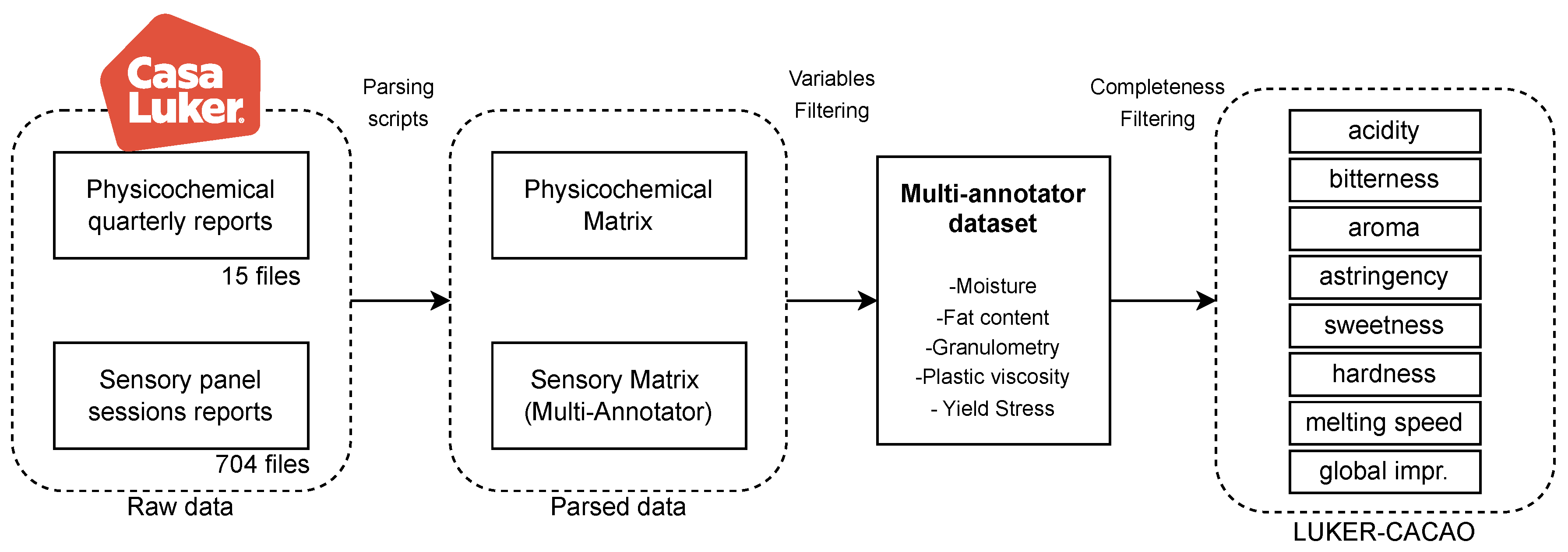
The original dataset was compiled from two distinct sources: 15 quarterly technical reports containing physicochemical measurements, and 704 sensory evaluation session files. The physicochemical data were obtained through standardized instrumental analyses, while the sensory sessions involved trained panelists who provided evaluations of cacao production samples according to established sensory protocols. To construct a unified and analyzable dataset, all reports were systematically parsed using automated data extraction pipelines. The relevant tabular data were consolidated into two structured matrices: one representing the physicochemical descriptors (input features) and the other capturing the sensory evaluations (multi-annotator outputs). The sensory matrix adopts a structured format in which each row corresponds to a product sample and each column represents a specific sensory descriptor provided by an individual annotator, reflecting the inherent variability and sparsity of crowd-sourced annotations.
A subset of variables from both data modalities was subsequently selected to ensure consistency and relevance. For the physicochemical domain, five variables were retained based on their completeness across samples and their potential to capture key aspects of product structure and composition:
- -
- Moisture: It refers to the amount of water present in a cocoa-based product, expressed as a percentage of the product’s total weight (%). Moisture content significantly impacts physical attributes such as texture, shelf-life, and microbial stability. More critically, it modulates the release and perception of flavor compounds during consumption. Variations in moisture influence the volatilization of aroma molecules and alter the way flavors are experienced in the mouth, thereby reshaping the sensory profile in terms of intensity, balance, and mouthfeel [32]. In the dataset, moisture values range from 0 to approximately 200%.
- -
- Fat content: It represents the proportion of lipids present in cocoa-based products, expressed as a percentage of total weight (%). Its modulation influences physical properties like viscosity, structure, and film formation capacity. These physical changes affect how the product interacts with the mouth during consumption, thereby altering the sensory profile by modifying lubrication, mouthfeel, and perception of flavor release [33]. In the dataset, values range from 0 to 60%.
- -
- Granulometry: It measures the size and distribution of solid particles in cocoa-based products, expressed in micrometers (m). Granulometry influences how particles interact and pack together, altering viscosity, flow behavior, and ultimately the perception of mouthfeel during consumption. Changes in granulometry reshape the sensory profile by modifying sensations like smoothness, thickness, and creaminess, which are critical for consumer acceptance [34]. Granulometry values range from 0 to 58 m.
- -
- Plastic viscosity: Measures the resistance of the product to flow after yielding has occurred, expressed in Pascal-seconds (Pa·s). It also reflects how easily the material continues to deform under applied shear during oral processing. Variations in plastic viscosity affect the sensory profile by altering the perceived thickness, smoothness, and creaminess during consumption. These changes shape the overall mouthfeel, influencing whether the product is experienced as rich, velvety, or fluid [34]. Observed values range from 0 to approximately 10.5 Pa·s.
- -
- Yield stress: Represents the minimum force required to initiate flow in the product, expressed in Pascals (Pa). It is closely related to the structural integrity of the product before deformation starts. Variations in yield stress affect the sensory profile by altering initial mouthfeel sensations such as firmness and body, shaping the consumer’s perception of texture at the start of consumption [34]. Yield stress values range from 0 to approximately 62 Pa.
Likewise, from the sensory domain, eight attributes were selected based on their relevance to flavor perception and the density of available annotations. These attributes represent core dimensions of sensory quality. In trained descriptive analysis of cocoa-based products, sensory attributes are evaluated by expert panels using intensity scales ranging from 1 (absence) to 10 (maximum perceived intensity). These attributes capture key sensory dimensions affecting product quality, processing control, and consumer acceptance [35]:
- -
- Acidity: It refers to the perception of sourness resulting from organic acids formed during fermentation. When present at appropriate levels, acidity can enhance brightness and complexity; however, excessive acidity is considered a defect, particularly in fine chocolate [36].
- -
- Bitterness: It reflects the presence of alkaloids (primarily theobromine) and polyphenols, compounds inherent to cocoa. While some degree of bitterness is characteristic and desirable, excessive levels can disrupt sensory balance and negatively impact consumer acceptance [37].
- -
- Aroma: It encompasses volatile compounds responsible for cocoa’s characteristic smells (fruity, floral, roasted), highly influenced by fermentation and roasting [32].
- -
- Astringency: It refers to the drying, puckering sensation caused by interactions between polyphenols and salivary proteins. While moderate astringency can contribute positively to mouthfeel and complexity, excessive levels are perceived as unpleasant and may negatively impact sensory acceptance. [37].
- -
- Sweetness: It reflects sugar content, critical to balancing bitterness and acidity for overall flavor harmony.
- -
- Hardness: It describes the resistance during biting or deformation, influenced by fat content, tempering, and particle size.
- -
- Melting speed: It reflects how quickly the product liquefies in the mouth, depending on fat composition and tempering. Faster melting generally enhances flavor release and mouthfeel [35].
- -
- Global impresssion: It summarizes overall product quality, integrating flavor, aroma, and texture into a single judgment.
Of note, the analytical procedures used to obtain these physicochemical and sensory measurements are standardized and traceable to established methods. Table 1 summarizes the official protocols used for each selected measurement type.
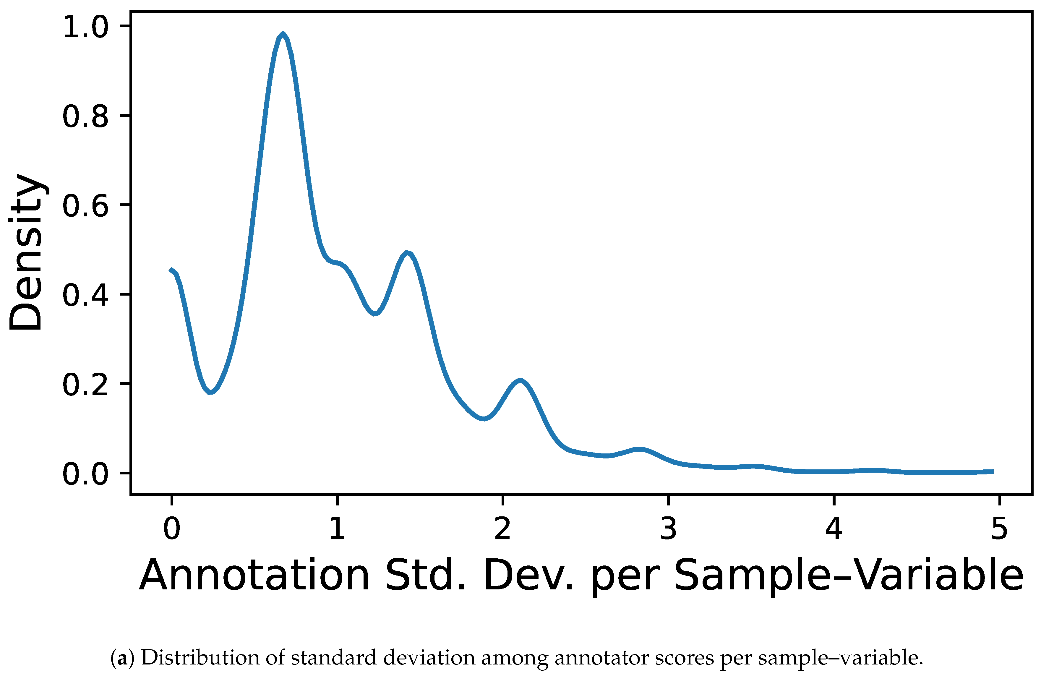
Next, to ensure adequate representation and consistency within the multi-annotator framework, the analysis was further restricted to a subset of five annotators, identified by the codes 135, 154, 155, 160, and 179. These annotators were selected based on their high annotation coverage across the chosen sensory attributes, enabling more reliable modeling of expert-specific patterns and behaviors. Namely, after merging we built an input–output, multi-annotator dataset with 1886 samples, five physicochemical features, and eight sensory outputs from five experts. Figure 1 presents the annotation coverage heatmap, grouping columns by sensory variable and ordering annotators within each block; black squares indicate present labels and white squares missing ones. This visualization highlights that certain variables include complete samples lacking annotations from any expert. Additionally, it reveals systematic patterns in annotator behavior—for instance, the fourth column in each block consistently shows fewer labels provided for attributes such as bitterness and aroma. Figure 3 further quantifies these patterns, providing a detailed overview of inconsistencies in annotator behavior: panel (a) shows the distribution of how many annotators labeled each sample—most receive labels from two to three experts—while panel (b) depicts the distribution of the standard deviation in annotator scores per sample–variable pair, revealing a concentration of low disagreement but also a long tail of cases with high annotator variability, emphasizing the challenge of modeling subjective sensory assessments.
For each selected sensory attribute, we constructed a dedicated dataset by intersecting the cleaned sensory and physicochemical records. The data were restricted to the previously selected subset of annotators and physicochemical features. To ensure that the learning models are trained on complete and reliable input–output pairs, we only retained samples that satisfied two conditions: (i) no more than one missing value among the physicochemical features, and (ii) no more than one missing annotation across the selected annotators for the target attribute.
This filtering strategy strikes a balance between strict completeness and reasonable sample retention, allowing us to preserve useful samples without compromising model integrity. Table 2 summarizes the percentage of available labels for each annotator across all sensory attributes. Table 3 shows the completeness of each physicochemical input feature, along with the final number of retained samples for each sensory regression task.
Figure 2.
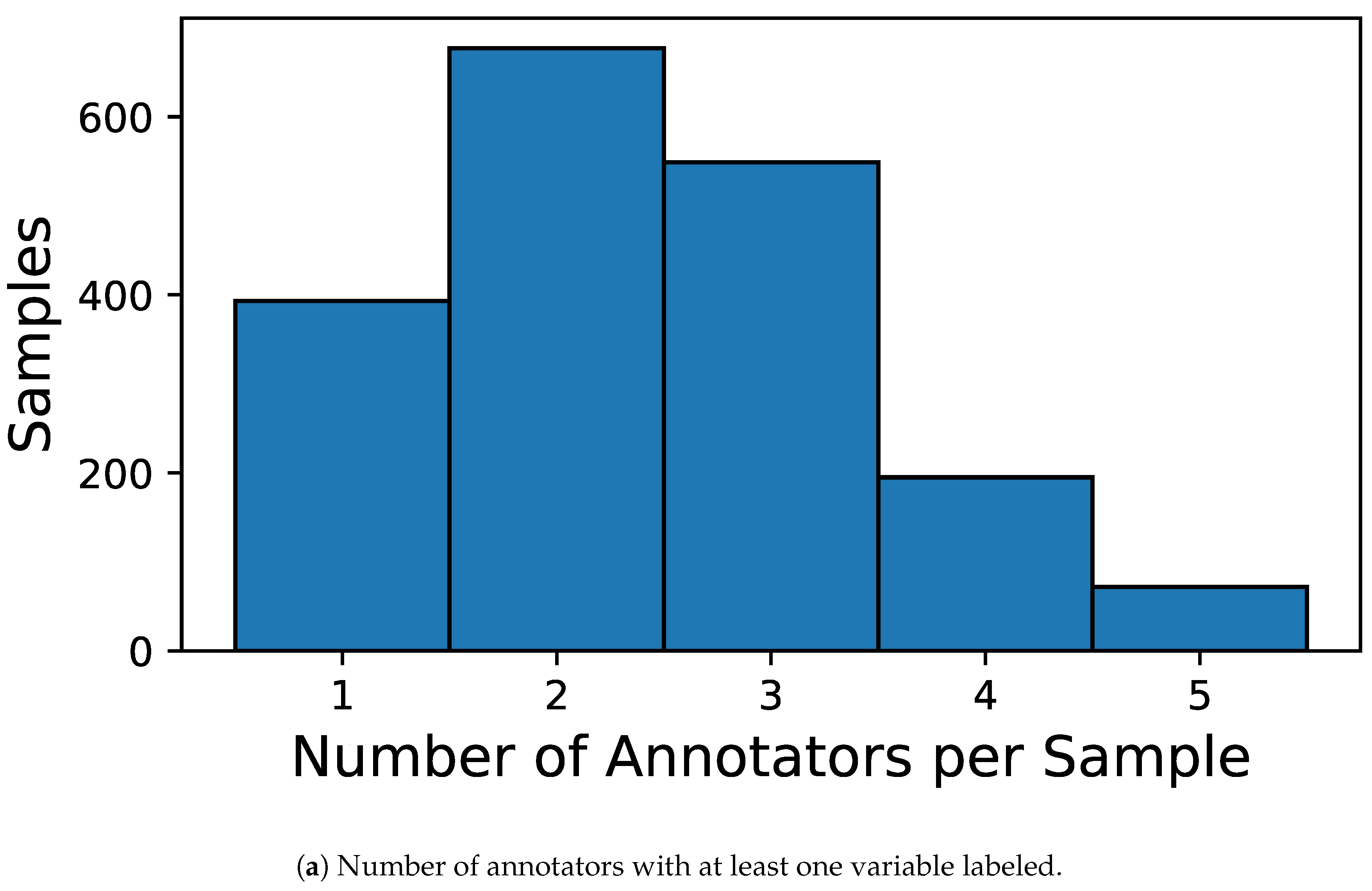
Figure 3.
Inconsistencies in annotator behavior. (a) Shows, for each sample, how many annotators provided at least one label across the eight sensory attributes, revealing a typical coverage of two to three annotators per sample.(b) Presents a kernel density estimate of the standard deviation in annotator scores for each sample–variable pair, quantifying how much annotators typically disagree. Most annotations exhibit standard deviations below 2.0, but a notable long tail indicates the presence of substantial inter-annotator variability in a subset of evaluations.
After applying the completeness constraints and constructing the final datasets for each sensory attribute, a final imputation step was performed to handle any remaining missing values in the physicochemical input variables. We employed the Iterative Imputer from scikit-learn, which estimates missing values by sequentially modeling each variable as a function of the others. This approach preserves inter-variable correlations and provides a flexible, data-driven completion method suitable for small datasets [43]. No imputation was applied to the sensory labels. Missing annotations were treated as unobserved and marginalized during training.
The overall data curation workflow is summarized in Figure 3. This diagram outlines the end-to-end process from raw data acquisition through parsing, variable selection, and completeness filtering, culminating in the construction of the LUKER-CACAO dataset. It highlights the progressive reduction and refinement of data needed to obtain high-quality, multi-annotator datasets suitable for learning reliable mappings between physicochemical properties and sensory perceptions.
Figure 4.
Pipeline for the construction of the LUKER-CACAO database.
2.2. Correlated Chained Gaussian Processes (CCGP)
Let a Gaussian Process (GP) be a collection of random variables indexed by the input samples such that any finite number of them follows a joint Gaussian distribution. Regarding this, a GP is completely specified by its mean ( for simplicity) and covariance , where is a kernel function, , and stands for the expectation operator [30]. Then: .
Now, let denote an input–output dataset consisting of N samples and P input features, where represents the input matrix and is the corresponding vector of continuous regression targets. We define the latent function evaluations over the dataset as , where , being a kernel matrix computed by evaluating the covariance function over all pairs of input points ().
Remarkably, GPs inherit the properties of multivariate Gaussian distributions, allowing for linear combinations of latent functions and facilitating the construction of additive models. When coupled with an appropriate link function, this framework can be naturally extended to accommodate non-Gaussian observation models, as in generalized linear model settings [44]. Moreover, in the general case of GP-based models for supervised learning, the observed data is modeled by constructing a joint distribution that combines a conditional likelihood with one or more latent functions governed by independent GP priors. If each parameter of the likelihood (e.g., noise variance, mean shift) is itself modeled as a latent function over the input space, the resulting structure is known as a Chained Gaussian Process (CGP) [45]. Formally, the joint distribution over and J latent functions (LFs) , conditioned on the input matrix , yields:
where the likelihood parameters , with , are nonlinear mappings from GP priors, e.g., , with mapping each to the appropriate domain . In addition, is an LF vector that follows a GP prior and is a kernel-based covariance matrix.
GPs, being nonparametric models, inherently scale poorly with dataset size due to their computational complexity of for a regression task defined over . To address this limitation, we adopt a widely used approximation strategy that introduces a set of inducing variables, denoted by , where . This sparse approximation reduces the computational cost of inference and learning to . Under this formulation, the CGP prior yields [46]:
Here, denotes the cross-covariance computed by evaluating between input samples and inducing points. Similarly, represents the covariance matrix between inducing points. By conditioning on the inducing variables , the marginal distribution over the latent function values is given by:
and the prior on is:
In general, the posterior distribution is intractable due to the non-conjugacy of the likelihood with respect to the priors (). Then, we approximate the posterior using variational inference with a parameterized distribution [23]:
where is a variational Gaussian distribution over the inducing variables and:
with and . These parameters are optimized by maximizing an Evidence Lower Bound (ELBO), which provides a tractable surrogate to the marginal likelihood. Assuming that the data points are independently and identically distributed, such an ELBO can be formulated as [47]:
where is the Kullback-Leibler divergence and .
Still, the standard CGP assumes independent GP priors for each likelihood parameter. The latter assumption is often unrealistic in multi-annotator scenarios, where annotators may share common biases or information sources [31]. To capture these dependencies, we employ a shared latent-factor structure [48]:
where , , and . Let be the sample-dependent model parameter vector, , , and herefore, the Correlated Chained Gaussian Process (CCGP) framework naturally emerges when the joint distribution in equation 1 is reformulated to explicitly model dependencies across outputs through a chained, conditionally correlated structure:
For each , we introduce pseudo-variables , by evaluating at . Likewise, , then:
where is block-diagonal, with computed from . The covariance matrix has elements .
Similarly, , where holds elements , with . Similar to the CGP, the posterior distribution of the CCGP, denoted as , is generally intractable in closed form. Consequently, it is approximated using a parameterized variational distribution, i.e., , following the approach in [23]:
where and . Besides, () and is a block-diagonal matrix holding covariance blocks We then approximate the joint posterior over all latent functions and their corresponding inducing variables using a factorized variational distribution. This approximation leads to the following ELBO:
where:
The first term in equation 13 encourages the variational posterior to explain the observed labels, while the second penalizes deviation from the GP prior over latent factors.
2.3. CCGP-based Crowd Learning and Localized Annotator Trustworthiness
Consider a multi-annotator dataset , where denotes the input features and is the corresponding label matrix provided by R annotators with unknown and potentially heterogeneous levels of expertise. The entry represents the label assigned by annotator r to the n-th sample. Since annotators may not label all samples, the matrix can contain missing values. Let denote the set of observed annotation indices. Then, for each , a label is observed, while for , the annotation is considered missing and excluded.
Here, we propose a CCGP-based crowd learning framework for multi-annotator regression tasks, referred to as MAR-CCGP. This approach is designed with two primary objectives: (i) to model each annotator’s performance as a localized function of the input space, thereby capturing annotator-specific trustworthiness across different regions; and (ii) to accurately infer the true label for a new input . Notably, the method operates in a fully unsupervised manner with respect to annotator reliability, no additional supervision regarding annotator expertise, experience, or consistency is assumed.
Conversely, for real-value outputs, we follow the multi-annotator approach in [49], where each is considered as a corrupted version of the estimated hidden ground truth , yielding:
where denotes the error variance associated with the r-th annotator for instance n. In our MAR-CCGP framework, each parameter of the likelihood in is linked to an LF , as defined in equation 8. Specifically, our model employs LFs: one dedicated to capturing the latent ground truth, and the remaining R to characterize the input-dependent error variances of each annotator:
where . Note that an exponential transformation is applied to the corresponding LF in equation 17 to ensure that the annotator-specific variance remains strictly positive, i.e., .
Afterward, an ELBO-based optmization from equation 13 is introduced for our MAR-CCGP, as follows:
where for denotes the variational marginal over the latent function values, as defined in equation 14; represents the variational distribution over the inducing variables (see equation 12); and corresponds to the GP prior over the inducing variables, given in equation 11.
In turn, given a new input sample , our goal is to compute the predictive mean and variance for both the estimated ground truth and the corresponding annotator-specific error variances . Specifically, as we defined the ground truth prediction as , the posterior distribution over is given by:
where:
Similarly, due to the exponential transformation in equation 17, the posterior distribution of the annotator-specific variance follows a log-normal distribution. Its parameters are determined by the predictive mean and variance in , yielding:
Finally, the proposed MAR-CCGP framework enables the assessment of localized annotator trustworthiness through a probabilistic reliability score derived from the model’s posterior predictions. For each annotator r and sample , the trustworthiness score is defined as:
where denotes the predicted ground truth for input sample , and is the estimated annotator-specific variance as in equations 20 and 22, respectively. The exponent modulates the sensitivity to the model’s predicted uncertainty, acting as a sublinear scaling factor. Setting was found to stabilize the trustworthiness score in regions of low predicted variance, preventing numerical explosions and yielding better alignment with empirical annotator behavior. This formulation corresponds to the scaled likelihood of the observed annotation under the model’s uncertainty, offering a principled, data-dependent trust metric for each annotator at a given input location.
3. Experimental Set-Up
To evaluate the effectiveness of the proposed MAR-CCGP framework in modeling information from multiple annotators, we conduct a series of experiments using both semi-synthetic and real-world datasets. The semi-synthetic benchmarks provide a controlled environment with access to ground-truth labels, enabling rigorous assessment of the model’s ability to infer annotator trustworthiness. In contrast, the real-world dataset—comprising sensory evaluations of cacao products (see the LUKER-CACAO dataset description in Section 2.1)—lacks ground-truth annotations, making it an ideal scenario to assess the framework’s capabilities in consensus estimation and uncertainty quantification.
3.1. Semi-Synthetic Datasets Annotation Simulation
We evaluate our MAR-CCGP approach under controlled conditions employing regression datasets from the University of California Irvine (UCI) machine learning repository(see https://archive.ics.uci.edu/datasets and Table 4). Each dataset provides continuous targets and input features, enabling the generation of simulated multi-annotator labels with structured noise profiles.
Moreover, to simulate annotator-specific variability, we adopt the following scheme:
- -
- The input data are standardized and then projected into a two-dimensional space using Uniform Manifold Approximation and Projection (UMAP) [50], to preserve local data structure by minimizing the cross-entropy between high-dimensional and low-dimensional fuzzy simplicial representations.
- -
- A K-means algorithm with C clusters is then applied to the UMAP projection to derive pseudo-contextual input space partitions [30], as latent indicators of instance-specific difficulty or domain shifts, used to modulate annotator behavior.
- -
- Let denote the cluster assignment associated with the input , and let represent the corresponding ground-truth regression value. The simulated label assigned by annotator r to instance n is then generated as follows:where is the annotator-specific error variance for cluster . To ensure interpretability and reproducibility, each annotator’s variance profile across clusters is defined in terms of a fixed Signal-to-Noise Ratio (SNR) in dB. Then, the multiple annotator target matrix for regression tasks , is built as in equation 25.
By varying the SNR across annotators and data clusters, we construct distinct variance profiles wherein certain annotators exhibit high reliability in specific regions of the input space and low reliability in others. This setup is intended to emulate real-world, non-stationary labeling behavior. For concreteness in our semi-synthetic data experiments, we fix the number of clusters to and the number of annotators to . The SNR values are varied according to the profiles shown in Figure 5. One annotator is designated as an expert, consistently exhibiting an SNR of across all data clusters.
3.2. Quality Assessment, Method Comparison, and Training Details
To evaluate whether the model-derived reliability scores accurately reflect annotator behavior, we aggregate both the predicted trustworthiness scores and empirical performance metrics across annotators and clusters. Specifically, for each annotator, we compute the average trustworthiness score within each cluster (see equation 24), defined as:
where denotes the set of input instances in cluster . For comparison, we compute the empirical coefficient of determination between annotator labels and model-predicted ground truth in the same regions:
where ∀
We benchmarked the proposed MAR-CCGP against three representative baselines, each embodying a distinct strategy for handling multi-annotator learning. As outlined in Table 5, the GPR-GT model serves as an optimistic upper bound, leveraging a GP regressor [30] trained directly on ground truth targets. This approach bypasses the inherent complexities of annotator-induced variability, thereby providing a best-case performance scenario. In contrast, the GPR-AVG represents a naive lower-bound reference, where annotations are averaged per instance to form pseudo-targets for GP training [23]. This method assumes uniform annotator reliability and fails to account for noise or systematic biases. A more nuanced alternative is offered by LKAAR, which simultaneously models annotator-specific noise and bias while learning an input-dependent reliability function via kernel alignment [31]. Notably, both LKAAR and our MAR-CCGP are among the few methods capable of modeling annotator consistency as a function of the input space.
Also, to quantitatively assess the predictive performance of the MAR-CCGP model for the semi-synthetic datasets, we include three standard regression measures: Mean Squared Error (MSE), Mean Absolute Error (MAE), and Mean Absolute Percentage Error (MAPE):
where is the true target (available in semi-synthetic scenarios) and is the predicted ground truth. is a small constant added to avoid division by zero when (set to in our experiments), denotes the sample mean of the ground truth values.

Table 5.
Comparative summary of baseline and advanced models for multi-annotator regression.
| Method | Acronym | Description |
|---|---|---|
| Gaussian Process on Ground Truth [30] | GPR-GT | Supervised GP regression trained on true outputs. Serves as an oracle upper bound and assumes full access to ground truth. Does not model annotators or uncertainty. |
| Gaussian Process on Average Annotations [23] | GPR-AVG | GP trained on the per-instance average of annotator targets. Assumes annotators are unbiased and neglects individual reliability. Serves as a baseline that models only the consensus. |
| Localized Kernel Alignment-based Annotator Relevance [31] | LKAAR | Jointly estimates annotator bias and variance, and embeds annotator consistency as a kernelized function over the input space. Provides localized reliability estimates. |
| Multi-Annotator Regression based on Correlated Chained Gaussian Process (ours) | MAR-CCGP | Proposed model. Captures latent inter-annotator correlations and input-dependent noise via correlated-chained latent functions and sparse variational GPs. Produces localized consistency-trustworthiness estimates. |
All experiments were conducted on the Kaggle platform using GPU-enabled notebooks. Each session provided access to a single NVIDIA Tesla P100 GPU (16GB VRAM), 30 GB of RAM, and 4 vCPUs from an Intel Xeon CPU @ 2.20GHz. The code-base was developed in Python 3.11.11, and all models were executed in the default Kaggle environment, with package versions listed in the notebook dependencies. Our MAR-CCGP model was implemented using GPflow 2.10.0 atop TensorFlow 2.18.0. Dimensionality reduction and clustering were handled by cuML 25.2.1 (RAPIDS), while preprocessing relied on scikit-learn 1.2.1. Additional tools included NumPy, Pandas, and Matplotlib for analysis and visualization.
All GP-based approaches and the regression components within LKAAR—used sparse variational inference with inducing points and a mini-batch size of 128. Inducing inputs were initialized via k-means clustering. A squared exponential kernel was used in all cases. Training was carried out using the Adam optimizer with a learning rate of for up to 1000 steps. If the ELBO did not improve for 20 consecutive iterations, the learning rate was halved to a minimum of . Early stopping was triggered if no improvement was observed over 500 iterations.
Each experiment was repeated over 15 randomized train/test splits (70/30). For the semi-synthetic datasets, splits were stratified by the UMAP-based cluster labels to preserve input-space diversity across folds. In the cacao-based real-world dataset (LUKER-CACAO), where no cluster labels were available, standard random splits were applied. Random seeds were fixed for all runs to ensure reproducibility. Code and full experiment notebooks for semi-synthetics datasets are publicly available at: https://github.com/UN-GCPDS/python-gcpds.luker_multiple_annotators. Access to the LUKER-CACAO dataset is restricted owing to copyright limitations established by the Casa Luker organization.
Figure 7.
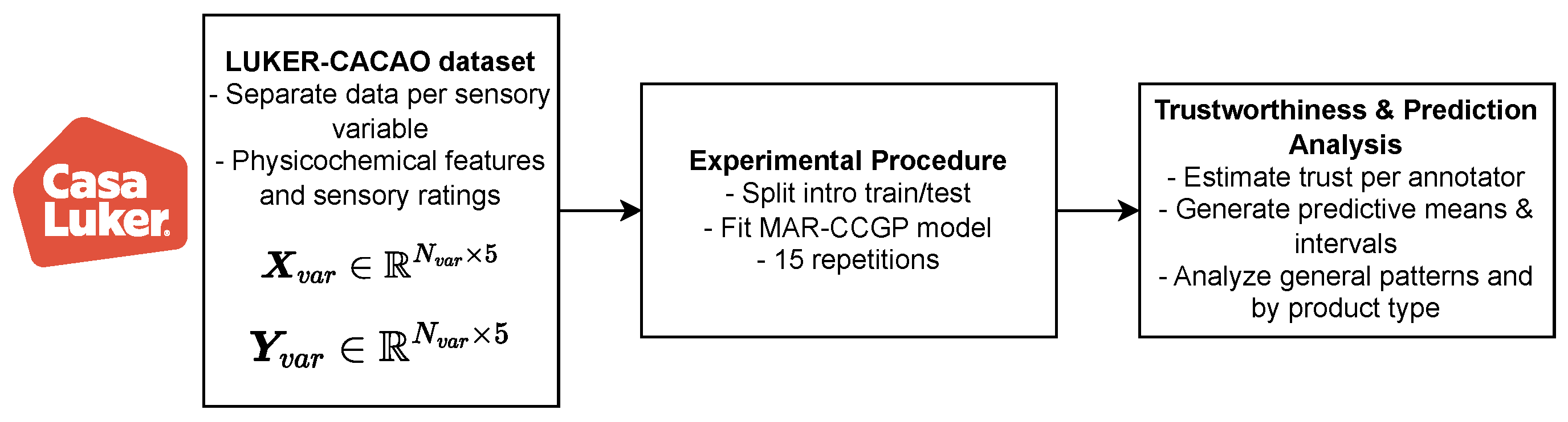
LUKER-CACAO dataset MAR-CCGP experimental set-up.
4. Results and Discussion
4.1. Semi-Synthetic Datasets Results
We first evaluate all models using the semisynthetic benchmark datasets described in Table 4. These datasets allow controlled experimentation with known ground truth, enabling a detailed assessment of both predictive accuracy and the quality of learned annotator reliability.
To simulate non-stationary annotator behavior, we followed the procedure outlined in Section 3.1. Ground truth labels were corrupted using structured noise profiles defined by a SNR matrix, assigning fixed reliability levels per annotator and input cluster. As shown in Figure 5, Annotator 1 is modeled as a consistent expert (SNR = 10 dB across all clusters), while Annotators 2–5 exhibit cluster-dependent behavior. For instance, Annotator 3 is highly accurate in Cluster 2 (6 dB) but unreliable in Cluster 1 (–3 dB), simulating realistic local variability in annotator performance. Figure 8 illustrates the UMAP-based clustering for the Bike Sharing dataset, and Figure 9 shows the resulting noisy annotations alongside the ground truth.
All models were evaluated over 15 randomized 70/30 train/test splits, stratified by the clusters used in the annotator simulation. We report the mean and standard deviation of test-set metrics: MSE, MAE, MAPE, and . Results are presented in Table 6.
Across all datasets, MAR-CCGP consistently achieves the best performance in terms of both error metrics (MSE, MAE, MAPE) and explanatory power (), highlighting its ability to model input-dependent annotator reliability and inter-annotator correlations. This advantage stems from its capacity to learn both latent ground truth and annotator noise structure jointly, leveraging the semi-parametric latent factor model and shared latent processes. GPR-GT, trained using uncorrupted ground truth, serves as a strong upper bound, yet MAR-CCGP often matches or approaches its performance—particularly in more complex datasets—despite only observing noisy annotations. In contrast, GPR-AVG, which averages noisy labels, suffers from bias introduced by context-dependent errors, yielding significantly higher error rates. LKAAR, while modeling local annotator reliability, fails to capture dependencies between annotators or fully account for the structured noise patterns, leading to lower predictive accuracy and less stable performance. These results support the hypothesis that modeling non-stationary, correlated annotation noise yields more robust predictors, even under limited and noisy supervision.
To evaluate MAR-CCGP’s ability to recover localized annotator trustworthiness, we applied the assessment framework described in Section 2.3. Specifically, for each dataset, we partitioned the input space into clusters and computed two cluster-level matrices: (1) the empirical coefficient of determination , which quantifies the agreement between each annotator’s labels and the inferred ground truth, and (2) the average localized trustworthiness score derived from the model’s posterior predictive distribution. These metrics enable a direct comparison between empirical annotator behavior and the model’s estimated reliability across different regions of the input space.
Figure 10 presents the cluster-wise empirical scores (left) alongside the corresponding MAR-CCGP trustworthiness estimates (right) for the Bike Sharing dataset. The left panel clearly shows that Annotator 1 is the most reliable across all clusters, achieving the highest in every region — as expected given its uniform SNR profile. MAR-CCGP’s estimated trustworthiness on the right reproduces this behavior closely, assigning consistently high trust scores to Annotator 1 across all clusters. In contrast, Annotators 2–5 exhibit substantial local variations: for instance, Annotator 2 is most accurate in Cluster 1 but becomes much less accurate in Clusters 3 and 4, and this is accurately reflected in its estimated trustworthiness profile. Similarly, Annotator 5 is most reliable in Cluster 4 (), which matches the model’s highest trustworthiness estimate () in that region. Overall, these heatmaps reveal a strong correspondence between empirical annotator performance and the model’s estimated reliability.
To quantify this alignment, we computed the squared Pearson correlation between the flattened empirical and model-derived trustworthiness matrices, obtaining a strong value of . This indicates that the model-internal trust estimates not only reflect qualitative trends but also align quantitatively with observed annotator behavior. Figure 11 further complements this analysis by visualizing per-sample trustworthiness across the input space, illustrating spatially localized patterns consistent with the annotator-specific noise profiles imposed during simulation.
To summarize these findings across all datasets, we averaged the cluster-wise scores per annotator, yielding the aggregated heatmaps shown in Figure 12. Annotator 1 emerges as consistently the most trustworthy across all datasets, exactly as simulated by its uniform SNR profile. This trend is well recovered by the MAR-CCGP model, which also correctly reflects the relative strengths and weaknesses of the remaining annotators. To quantify this overall alignment, we computed the squared Pearson correlation between the flattened empirical and model-estimated trustworthiness scores across all datasets, obtaining a high value of . This strong correspondence underlines the proposed method’s effectiveness in capturing true annotator behaviors even under diverse, noisy conditions, and confirms that MAR-CCGP provides robust, input-dependent trustworthiness estimates that closely match empirical annotator reliability.
4.2. LUKER-CACAO Dataset Results
Having demonstrated the predictive performance and trustworthiness inference capabilities of MAR-CCGP on semi-synthetic data, we now turn to a real-world application using the LUKER-CACAO dataset described in Section 2.1. Unlike the controlled benchmarks, this sensory evaluation dataset contains separate, curated input–output tables for each of eight sensory attributes (acidity, bitterness, aroma, astringency, sweetness, hardness, melting speed, and global impression), along with physicochemical features measured per sample (moisture, fat content, granulometry, plastic viscosity, yield stress). Importantly, the dataset contains ratings from five annotators without ground-truth labels, making this an ideal setting for MAR-CCGP to estimate a consensus profile and explore localized annotator trustworthiness.
Following the same experimental setup as the semi-synthetic case (training and testing over 15 random repetitions with 70/30 splits), we applied MAR-CCGP to each sensory variable separately. This setup enables a fair and consistent comparison across attributes and ensures that observed trends reflect annotator behavior rather than sampling variability.
Figure 13 shows the estimated mean sweetness profile learned by the model across all samples, along with its 95% predictive credible intervals. Individual annotator ratings are overlaid for direct comparison. The model’s mean estimate lies centrally among the noisy annotator ratings, especially where agreement is high, and predictive intervals widen in the left-hand region of the plot where annotators strongly disagree. Conversely, intervals narrow as ratings converge at higher sweetness levels, demonstrating the model’s ability to represent both consensus and uncertainty appropriately.
To further explore annotator-specific behavior, we investigated correlations between physicochemical properties and MAR-CCGP–inferred trustworthiness scores. Figure 14 presents a bipartite graph of these relationships. Nodes on the left represent the five physicochemical features, while nodes on the right represent the five annotators. Edge color indicates the Pearson correlation between a feature’s value and an annotator’s estimated trustworthiness across all samples. Warm edges show positive correlations and cool edges show negative correlations. The graph reveals that several annotators—most notably 154 and 160—exhibit negative correlations with fat content and moisture, suggesting that as these features increase, sweetness ratings become less reliable for these annotators. This is consistent with the intuition that fat and moisture may mask sweetness perception. Conversely, granulometry and yield stress show weaker or even positive correlations for some annotators (e.g. Annotator 135), implying that these panelists evaluate sweetness more reliably under these physical conditions.
To visualize trustworthiness across the physicochemical input space, Figure 15 depicts UMAP projections of the cacao samples, color-coded by MAR-CCGP’s estimated trustworthiness per annotator. The top-left panel depicts the estimated mean sweetness profile projected into the UMAP space, serving as a baseline. The remaining panels show each annotator’s trust scores across this space. Annotators 154 and 155 achieve high trustworthiness across most regions (consistently warm yellow hues), indicating stable and reliable performance. Annotators 160 and 179, by contrast, display region-specific drops in trustworthiness, especially for clusters of samples with high moisture or fat content. These localized patterns highlight systematic variations in annotator behavior across product types.
Finally, Table 7 and Figure 16 provide a detailed summary of estimated annotator trustworthiness across all sensory variables and product types. Consistent with the qualitative UMAP patterns, Annotators 154 and 155 stand out as the most consistently trustworthy panelists, yielding mean trust scores above for most attributes with low standard deviations across different product types. This is evident not only in sweetness but also for aroma, melting speed, hardness, and global impression, where both annotators maintain strong and stable reliability. Annotator 160, by contrast, exhibits markedly lower mean trustworthiness across many attributes (typically in the – range), with larger standard deviations — especially for perceptually challenging attributes like astringency and bitterness — indicating highly variable performance that depends on the product’s physicochemical profile. Annotator 179 also shows a similar pattern of reduced consistency, attaining good trust scores for a few localized product types but generally underperforming relative to the most consistent annotators. Interestingly, some sensory variables, such as bitterness and astringency, present inherently greater variability in trust scores across all panelists, suggesting that these attributes may be more difficult to evaluate reliably across the diverse product set. In contrast, more mechanically defined properties like hardness and melting speed exhibit higher and more uniform trustworthiness estimates across all annotators, which could reflect the greater perceptual salience of these sensory dimensions. Taken together, these findings demonstrate that MAR-CCGP successfully disentangles systematic annotator-specific behavior from product-specific effects, yielding granular trustworthiness estimates that highlight where particular panelists excel or struggle. This level of insight can inform sensory panel calibration, personalized training, and targeted quality control by drawing attention to specific attributes and product types that require additional guidance or closer monitoring.
Together, these findings demonstrate MAR-CCGP’s capacity to extract nuanced, input-dependent trustworthiness estimates even in real-world sensory settings without ground-truth supervision. The model’s trust scores closely align with expected behavior derived from physicochemical features, and its uncertainty estimates highlight regions where panel agreement is weakest. Importantly, these insights offer actionable guidance for panelist training and calibration, allowing sensory scientists to identify panelists who struggle with specific product types and potentially target these areas for further calibration or retraining.
4.3. Limitations
While the MAR-CCGP framework provides a robust solution for integrating multi-annotator sensory data with physicochemical profiles, several limitations remain. First, the model assumes that annotator reliability can be effectively captured through input-dependent variance, which may oversimplify annotators’ behavior in scenarios involving complex biases or strategic labeling. Second, the proposed trustworthiness score relies on probabilistic estimations derived from model outputs, but its interpretation may be challenging in the absence of external validation mechanisms or behavioral ground truth. Moreover, although the method performs well in semi-synthetic and real-world settings, it is currently limited to low-dimensional input spaces with a manageable number of annotators; scalability to high-dimensional sensory domains or crowd-scale scenarios may require further optimization or approximation strategies. Additionally, the framework depends on Gaussian process inference, which incurs high computational costs as the dataset size increases. Finally, while the LUKER-CACAO dataset enables a valuable real-world demonstration, its proprietary nature restricts reproducibility and broader benchmarking by the community.
5. Conclusions
We introduce a Multi-Annotator Regression framework based on Correlated Chained Gaussian Processes, named MAR-CCGP, a novel multi-annotator approach that jointly models continuous sensory scores and input-dependent annotator reliability through a probabilistic Gaussian Process formulation. The key conceptual innovation lies in disentangling true perceptual signals from annotator-specific noise using a latent consensus function and localized trust estimation. Unlike previous methods that assume uniform or global annotator performance, MAR-CCGP learns region-specific annotator trustworthiness scores, enabling interpretability and robustness in the face of sparse, noisy, and subjective supervision. The model is particularly suited for domains like food science, where expert annotations are limited and often exhibit contextual biases.
Our results demonstrate the effectiveness of MAR-CCGP across both real-world and semi-synthetic settings. On the proprietary LUKER-CACAO dataset, the model achieved strong predictive performance for multiple sensory attributes and provided meaningful trust scores that aligned with empirical annotator behavior, especially in dimensions such as bitterness and aroma. In controlled experiments with structured SNR profiles, MAR-CCGP outperformed consensus-only and local-weighting baselines in both RMSE and reliability estimation. Importantly, the model’s ability to recover annotator-specific patterns in low-trust clusters highlights its utility in curating more reliable datasets and guiding future annotation efforts. These findings suggest that MAR-CCGP not only enhances regression accuracy under label noise but also supports informed decision-making through interpretable reliability scores.
Future research could explore scaling MAR-CCGP to high-dimensional input domains and larger annotator pools by integrating sparse approximations or deep kernel learning methods [51,52]. Another promising direction involves extending the framework to heteroscedastic multi-output settings, allowing the simultaneous modeling of correlations between multiple sensory targets and annotator behaviors. Incorporating behavioral signals or auxiliary metadata from annotators—such as labeling time, confidence, or experience level—could further refine trust estimation [53,54]. Lastly, validating the trust scores through longitudinal studies or expert-in-the-loop experiments may reinforce their adoption in high-stakes domains such as medical diagnostics, environmental monitoring, and consumer preference modeling.
Author Contributions
Conceptualization, J.L.-R. and A.A.-M.; data curation, M.C.-M., S.F.-G., and J.L.-R; methodology, J.L.-R., A.A.-M. and G.C.-D.; project administration, M.C.-M., S.F.-G., A.A.-M., and G.C.-D.; supervision, A.A.-M. and G.C.-D.; resources, J.L.-R. and A.A.-M. All authors have read and agreed to the published version of the manuscript.
Funding
Under grants provived by the project: "Prototipo funcional de lengua electrónica para la identificación de sabores en cacao fino de origen colombiano”, funded by Minciencias-82729-ICETEX 2022-0740 and Casa Luker.
Data Availability Statement
Semi-synthetics datasets are publicly available at: https://github.com/UN-GCPDS/python-gcpds.luker_multiple_annotators (accessed on 1 April 2025). Access to the LUKER-CACAO dataset is restricted due to copyright limitations.
Conflicts of Interest
The authors declare no conflicts of interest.
References
- Betancourt-Sambony, F.; Barrios-Rodríguez, Y.F.; Medina-Orjuela, M.E.; Amorocho Cruz, C.M.; Carranza, C.; Girón Hernández, L.J.; et al. Relationship between physicochemical properties of roasted cocoa beans and climate patterns: Quality and safety implications. LWT-Food Science and Technology 2025, 216. [CrossRef]
- Fanning, E.; Eyres, G.; Frew, R.; Kebede, B. Linking cocoa quality attributes to its origin using geographical indications. Food Control 2023, 151, 109825. [CrossRef]
- González-Orozco, C.E.; Porcel, M.; Yockteng, R.; Caro-Quintero, A.; Rodriguez-Medina, C.; Santander, M.; Zuluaga, M.; Soto, M.; Rodriguez Cortina, J.; Vaillant, F.E.; et al. Integrating new variables into a framework to support cacao denomination of origin: A case study in Southwest Colombia. Journal of the Science of Food and Agriculture 2024, 104, 1367–1381. [CrossRef] [PubMed]
- N. Suh, N.; F. Njimanted, G.; Thalut, N. Effect of farmers’ management practices on safety and quality standards of cocoa production: A structural equation modeling approach. Cogent Food & Agriculture 2020, 6, 1844848.
- Dos Santos, R.M.; Silva, N.M.d.J.; Moura, F.G.; Lourenço, L.d.F.H.; Souza, J.N.S.d.; Sousa de Lima, C.L. Analysis of the sensory profile and physical and physicochemical characteristics of amazonian cocoa (Theobroma cacao L.) beans produced in different regions. Foods 2024, 13, 2171. [CrossRef] [PubMed]
- Palma-Morales, M.; Rune, C.J.B.; Castilla-Ortega, E.; Giacalone, D.; Rodríguez-Pérez, C. Factors affecting consumer perception and acceptability of chocolate beverages. LWT 2024, 201, 116257. [CrossRef]
- Spataro, F.; Rosso, F.; Peraino, A.; Arese, C.; Caligiani, A. Key molecular compounds for simultaneous origin discrimination and sensory prediction of cocoa: An UHPLC-HRMS sensomics approach. Food Chemistry 2025, 463, 141201. [CrossRef]
- León-Inga, A.M.; Velásquez, S.; Quintero, M.; Taborda, N.; Cala, M.P. Effects of ultrafiltration membrane processing on the metabolic and sensory profiles of coffee extracts. Food Chemistry 2024, 451, 139396. [CrossRef]
- Herrera-Rocha, F.; Fernández-Niño, M.; Duitama, J.; Cala, M.P.; Chica, M.J.; Wessjohann, L.A.; Davari, M.D.; Barrios, A.F.G. FlavorMiner: a machine learning platform for extracting molecular flavor profiles from structural data. Journal of cheminformatics 2024, 16, 1–12. [CrossRef]
- Mota-Gutierrez, J.; Ferrocino, I.; Giordano, M.; Suarez-Quiroz, M.L.; Gonzalez-Ríos, O.; Cocolin, L. Influence of taxonomic and functional content of microbial communities on the quality of fermented cocoa pulp-bean mass. Applied and Environmental Microbiology 2021, 87, e00425–21. [CrossRef]
- Cantini, C.; Salusti, P.; Romi, M.; Francini, A.; Sebastiani, L. Sensory profiling and consumer acceptability of new dark cocoa bars containing Tuscan autochthonous food products. Food science & nutrition 2018, 6, 245–252.
- Collazos-Escobar, G.A.; Barrios-Rodríguez, Y.F.; Bahamón-Monje, A.F.; Gutiérrez-Guzmán, N. Mid-infrared spectroscopy and machine learning as a complementary tool for sensory quality assessment of roasted cocoa-based products. Infrared Physics & Technology 2024, 141, 105482.
- Yadav, S.; Singh, A.; Kumar, N. Electronic panel for sensory assessment of food: A review on technologies integration and their benefits. Journal of Food Science 2025, 90, e70128. [CrossRef]
- Putri, D.N.; De Steur, H.; Juvinal, J.G.; Gellynck, X.; Schouteten, J.J. Sensory attributes of fine flavor cocoa beans and chocolate: A systematic literature review. Journal of Food Science 2024, 89, 1917–1943. [CrossRef] [PubMed]
- An, J.; Lee, J. Consumers’ sensory perception homogeneity and liking of chocolate. Food Quality and Preference 2024, 118, 105178. [CrossRef]
- Shawky, E.; Zhu, W.; Tian, J.; Abu El-Khair, R.A.; Selim, D.A. Metabolomics-Driven Prediction of Vegetable Food Metabolite Patterns: Advances in Machine Learning Approaches. Food Reviews International 2025, 41, 1051–1080. [CrossRef]
- Khonina, S.N.; Kazanskiy, N.L.; Oseledets, I.V.; Nikonorov, A.V.; Butt, M.A. Synergy between artificial intelligence and hyperspectral imagining—A review. Technologies 2024, 12, 163. [CrossRef]
- Mahanti, N.K.; Shivashankar, S.; Chhetri, K.B.; Kumar, A.; Rao, B.B.; Aravind, J.; Swami, D. Enhancing food authentication through E-nose and E-tongue technologies: Current trends and future directions. Trends in Food Science & Technology 2024, p. 104574.
- Taheri, S.; Andrade, J.C.d.; Conte-Junior, C.A. Emerging perspectives on analytical techniques and machine learning for food metabolomics in the era of industry 4.0: a systematic review. Critical Reviews in Food Science and Nutrition 2024, pp. 1–27.
- Gil-González, J.; Daza-Santacoloma, G.; Cárdenas-Peña, D.; Orozco-Gutiérrez, A.; Álvarez-Meza, A. Generalized cross-entropy for learning from crowds based on correlated chained Gaussian processes. Results in Engineering 2025, 25. [CrossRef]
- Raykar, V.C.; Yu, S.; Zhao, L.H.; Valadez, G.H.; Florin, C.; Bogoni, L.; Moy, L. Learning from crowds. Journal of Machine Learning Research 2010, 11, 1297–1322.
- Zhang, Y.; Li, X.; Zhang, T.; et al.. A survey on learning from noisy labels. IEEE Transactions on Pattern Analysis and Machine Intelligence 2022.
- Gil-Gonzalez, J.; Giraldo, J.J.; Orozco-Gutierrez, A. Correlated chained Gaussian processes for datasets with multiple annotators. IEEE Transactions on Neural Networks and Learning Systems 2021, 34, 4514–4528. [CrossRef] [PubMed]
- Rodrigues, F.; Pereira, F. Deep learning from crowds. In Proceedings of the AAAI, 2018.
- Zhang, Y.; Sheng, V.S. Learning from crowdsourced data with noise and annotation sparsity. In Proceedings of the IJCAI, 2016.
- Zhang, Z.; Sabuncu, M.R. Generalized cross entropy loss for training deep neural networks with noisy labels. NeurIPS 2018.
- Booth, B.M.; Narayanan, S.S. Fifty shades of green: Towards a robust measure of inter-annotator agreement for continuous signals. In Proceedings of the Proceedings of the 2020 international conference on multimodal interaction, 2020, pp. 204–212.
- Schilling, M.; Scherr, T.; Münke, F.; Neumann, O. Automated annotator variability inspection for biomedical image segmentation. IEEE Transactions on Medical Imaging 2022. [CrossRef]
- Atcheson, M.; Sethu, V.; Epps, J. Demonstrating and Modelling Systematic Time-varying Annotator Disagreement in Continuous Emotion Annotation. In Proceedings of the Interspeech, 2018.
- Murphy, K.P. Probabilistic machine learning: an introduction; MIT press, 2022.
- Gil-Gonzalez, J.; Orozco-Gutierrez, A.; Álvarez-Meza, A. Learning from multiple inconsistent and dependent annotators to support classification tasks. Neurocomputing 2021, 423, 236–247. [CrossRef]
- Aprotosoaie, A.C.; Luca, S.V.; Miron, A. Flavor chemistry of cocoa and cocoa products—an overview. Comprehensive Reviews in Food Science and Food Safety 2016, 15, 73–91. [CrossRef]
- Meza, B.E.; Carboni, A.D.; Peralta, J.M. Water adsorption and rheological properties of full-fat and low-fat cocoa-based confectionery coatings. Food and Bioproducts Processing 2018, 110, 16–25. [CrossRef]
- Principato, L.; Carullo, D.; Gruppi, A.; Lambri, M.; Bassani, A.; Spigno, G. Correlation of rheology and oral tribology with sensory perception of commercial hazelnut and cocoa-based spreads. Journal of Texture Studies 2024, 55, e12850. [CrossRef] [PubMed]
- Beckett, S.T.; Fowler, M.S.; Ziegler, G.R. Beckett’s industrial chocolate manufacture and use; John Wiley & Sons, 2017.
- Afoakwa, E.O.; Paterson, A.; Fowler, M.; Ryan, A. Flavor formation and character in cocoa and chocolate: a critical review. Critical reviews in food science and nutrition 2008, 48, 840–857. [CrossRef]
- Colonges, K.; Seguine, E.; Saltos, A.; Davrieux, F.; Minier, J.; Jimenez, J.C.; Lahon, M.C.; Calderon, D.; Subia, C.; Sotomayor, I.; et al. Diversity and determinants of bitterness, astringency, and fat content in cultivated Nacional and native Amazonian cocoa accessions from Ecuador. The Plant Genome 2022, 15, e20218. [CrossRef]
- AOAC International. AOAC Official Method 963.15: Fat (Crude) in Cacao Products, 2019. Available at: https://www.aoac.org.
- AOAC International. AOAC Official Method 931.04: Moisture in Cocoa Products, 2019. Available at: https://www.aoac.org.
- International Organization for Standardization. ISO 13320:2020 Particle size analysis—Laser diffraction methods, 2020. Available at: https://www.iso.org.
- International Office of Cocoa, Chocolate and Confectionery. IOCCC Analytical Method 46: Viscosity of Cocoa and Chocolate, 2000. Available at: https://www.ioccc.org.
- ICONTEC. NTC 3932: Sensory Analysis – Identification and selection of descriptors to establish a sensory profile using a multidimensional approach, 2004. Available at: https://www.icontec.org.
- Azur, M.J.; Stuart, E.A.; Frangakis, C.; Leaf, P.J. Multiple imputation by chained equations: what is it and how does it work? International journal of methods in psychiatric research 2011, 20, 40–49. [CrossRef]
- Williams, C.; Rasmussen, C. Gaussian processes for regression. Advances in neural information processing systems 1995, 8.
- Saul, A.D.; Hensman, J.; Vehtari, A.; Lawrence, N.D. Chained gaussian processes. In Proceedings of the Artificial intelligence and statistics. PMLR, 2016, pp. 1431–1440.
- Titsias, M. Variational learning of inducing variables in sparse Gaussian processes. In Proceedings of the Artificial intelligence and statistics. PMLR, 2009, pp. 567–574.
- Gal, Y.; van der Wilk, M. Variational Inference in Sparse Gaussian Process Regression and Latent Variable Models – A Gentle Tutorial, 2014, [arXiv:stat.ML/1402.6842]. arXiv:1402.6842. arXiv:1402.6842.
- Teh, Y.W.; Seeger, M.; Jordan, M.I. Semiparametric latent factor models. In Proceedings of the International Workshop on Artificial Intelligence and Statistics. PMLR, 2005, pp. 333–340.
- Rodrigues, F.; Lourenco, M.; Ribeiro, B.; Pereira, F.C. Learning supervised topic models for classification and regression from crowds. IEEE transactions on pattern analysis and machine intelligence 2017, 39, 2409–2422. [CrossRef] [PubMed]
- Healy, J.; McInnes, L. Uniform manifold approximation and projection. Nature Reviews Methods Primers 2024, 4, 82. [CrossRef]
- Wilson, A.G.; Hu, Z.; Salakhutdinov, R.; Xing, E.P. Deep kernel learning. In Proceedings of the Advances in neural information processing systems, 2016, Vol. 29, pp. 3703–3711.
- Salimbeni, H.; Deisenroth, M.P. Doubly stochastic variational inference for deep Gaussian processes. In Proceedings of the Advances in neural information processing systems, 2017, Vol. 30, pp. 4588–4599.
- Nguyen, K.; Yao, A.; Rezatofighi, H.; Shen, C.; Li, B. Confidence-Aware Learning from Noisy Labels. In Proceedings of the International Conference on Learning Representations (ICLR), 2022.
- Han, B.; Guo, Y.; Liu, D.; Gong, M.; Tao, D. TRAS: Trusted Labeling for Noisy Student Training. In Proceedings of the Proceedings of the IEEE/CVF Conference on Computer Vision and Pattern Recognition (CVPR), 2021, pp. 10200–10209.
Figure 1.
Annotation coverage heatmap across samples (rows) and eight sensory variables (columns). Columns are grouped by variable, and within each group the annotators are sorted (left-to-right: IDs 135, 154, 155, 160, 179).Black cells denote an annotation present; white cells denote missing annotations.Note that for several variables (e.g. acidity, astringency), there are entire samples with no labels from any annotator, and specific annotators (e.g. annotator 160, the fourth column in each block) show markedly lower coverage on variables like bitterness and aroma.
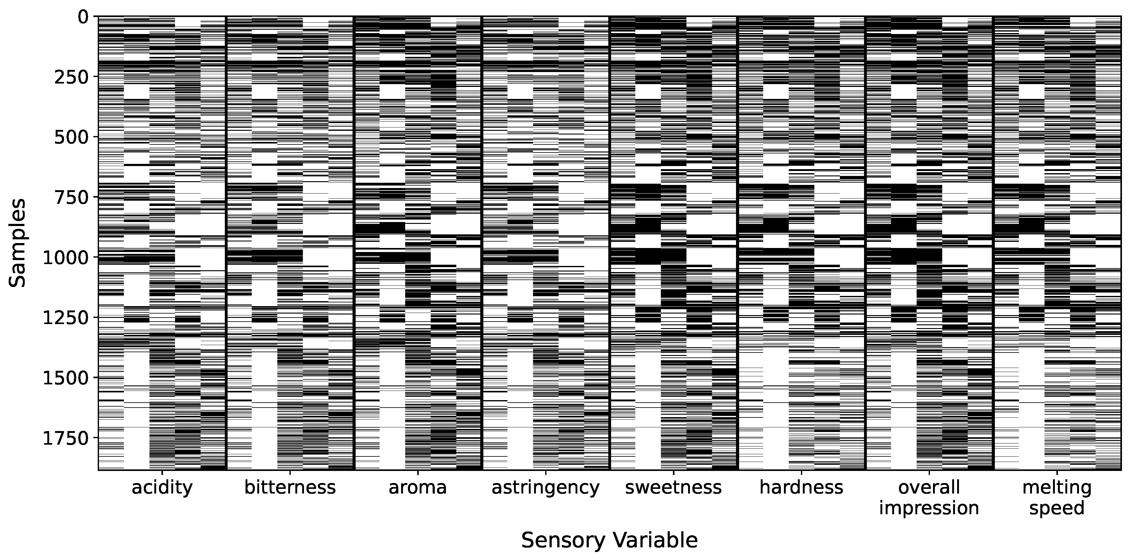
Figure 5.
Signal-to-Noise Ratio (SNR, in dB) matrix used in the semi-synthetic annotation simulation to model annotator-specific variance across clusters. Annotator 1 serves as a uniformly reliable expert, while the remaining annotators exhibit cluster-dependent variability in labeling accuracy.
Figure 5.
Signal-to-Noise Ratio (SNR, in dB) matrix used in the semi-synthetic annotation simulation to model annotator-specific variance across clusters. Annotator 1 serves as a uniformly reliable expert, while the remaining annotators exhibit cluster-dependent variability in labeling accuracy.
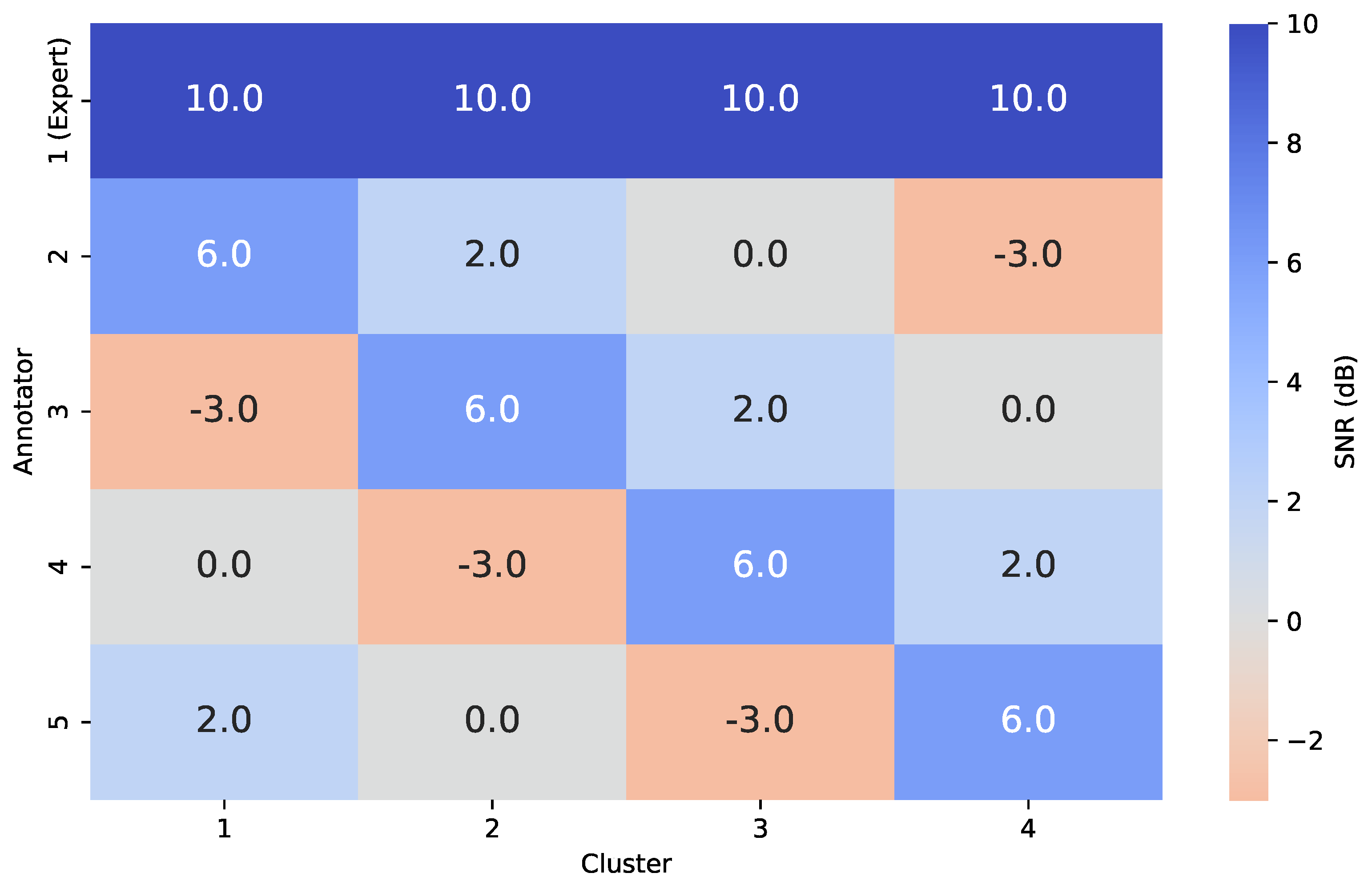
Figure 6.
Semi-synthetic datasets MAR-CCGP experimental set-up.
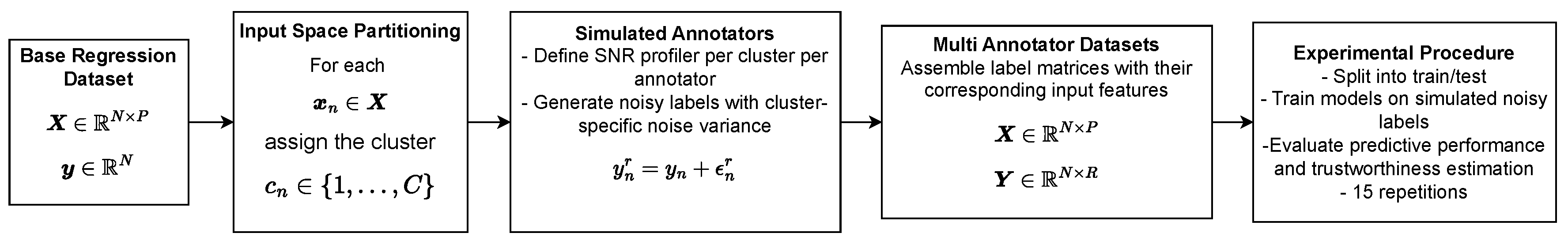
Figure 8.
UMAP 2D projection and k-means clustering of the Bike Sharing dataset. Each color represents a distinct cluster used to define local annotation noise patterns in the simulation process.
Figure 8.
UMAP 2D projection and k-means clustering of the Bike Sharing dataset. Each color represents a distinct cluster used to define local annotation noise patterns in the simulation process.
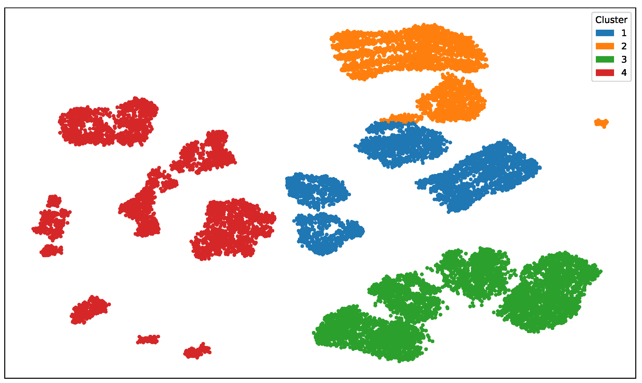
Figure 9.
Simulated multi-annotator labels for a subset of the Bike Sharing dataset. The solid black line represents the true target values, while each color-coded scatter indicates the noisy annotations from five simulated annotators. Samples are sorted by cluster to highlight regional reliability patterns: consistent deviations from the ground truth reveal how annotator accuracy varies across input regions, as defined by the SNR matrix.
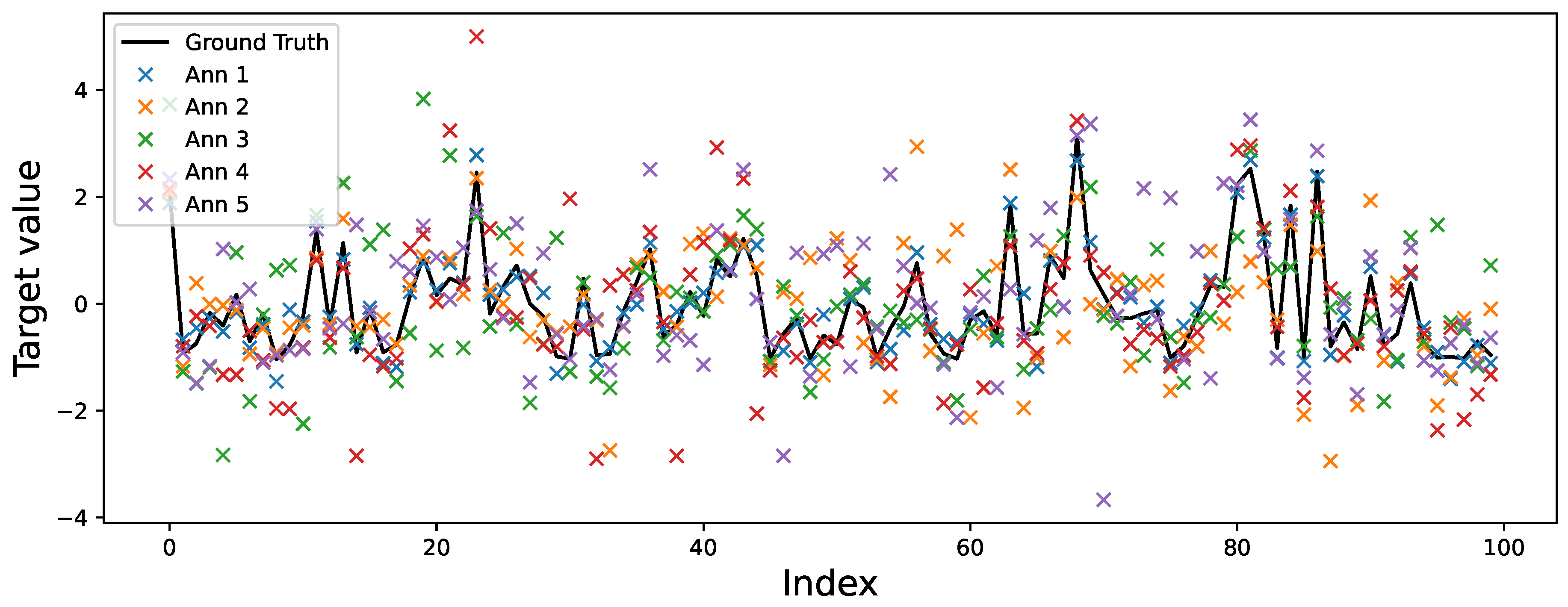
Figure 10.
Annotator trustworthiness for the Bike Sharing dataset. Left: Empirical scores between annotator labels and model-inferred ground truth, per cluster. Right: MAR-CCGP-derived trustworthiness scores per annotator and cluster. The model captures both global expertise (Annotator 1) and cluster-dependent variability.
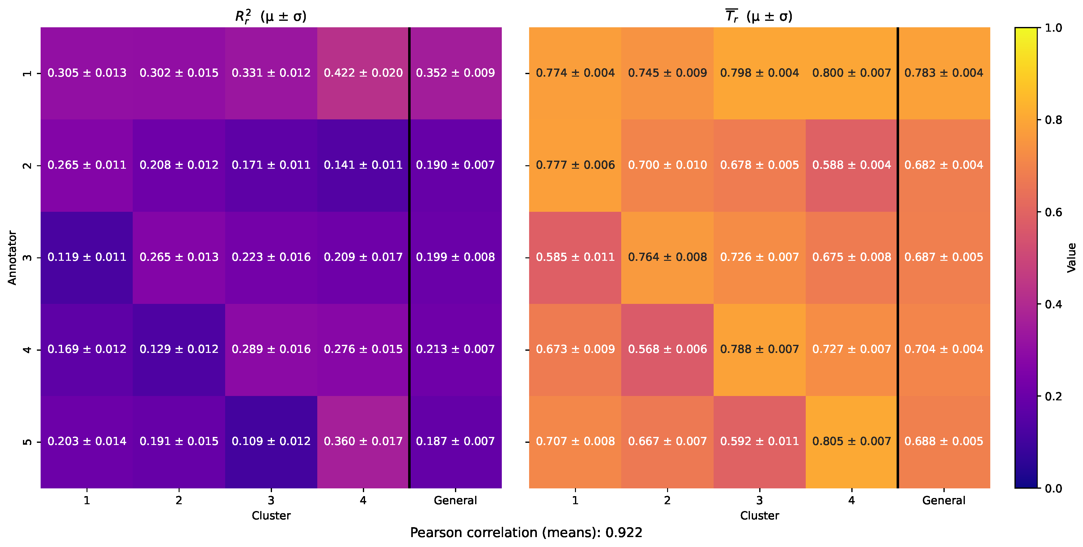
Figure 11.
Per-sample estimated reliability scores from MAR-CCGP for the Bike Sharing dataset. The top-left panel shows the true (uncorrupted) labels; subsequent panels show the predicted reliability of each annotator across samples. Annotator 1 is reliably trusted across the input space, while others display context-sensitive patterns consistent with the simulation SNR.
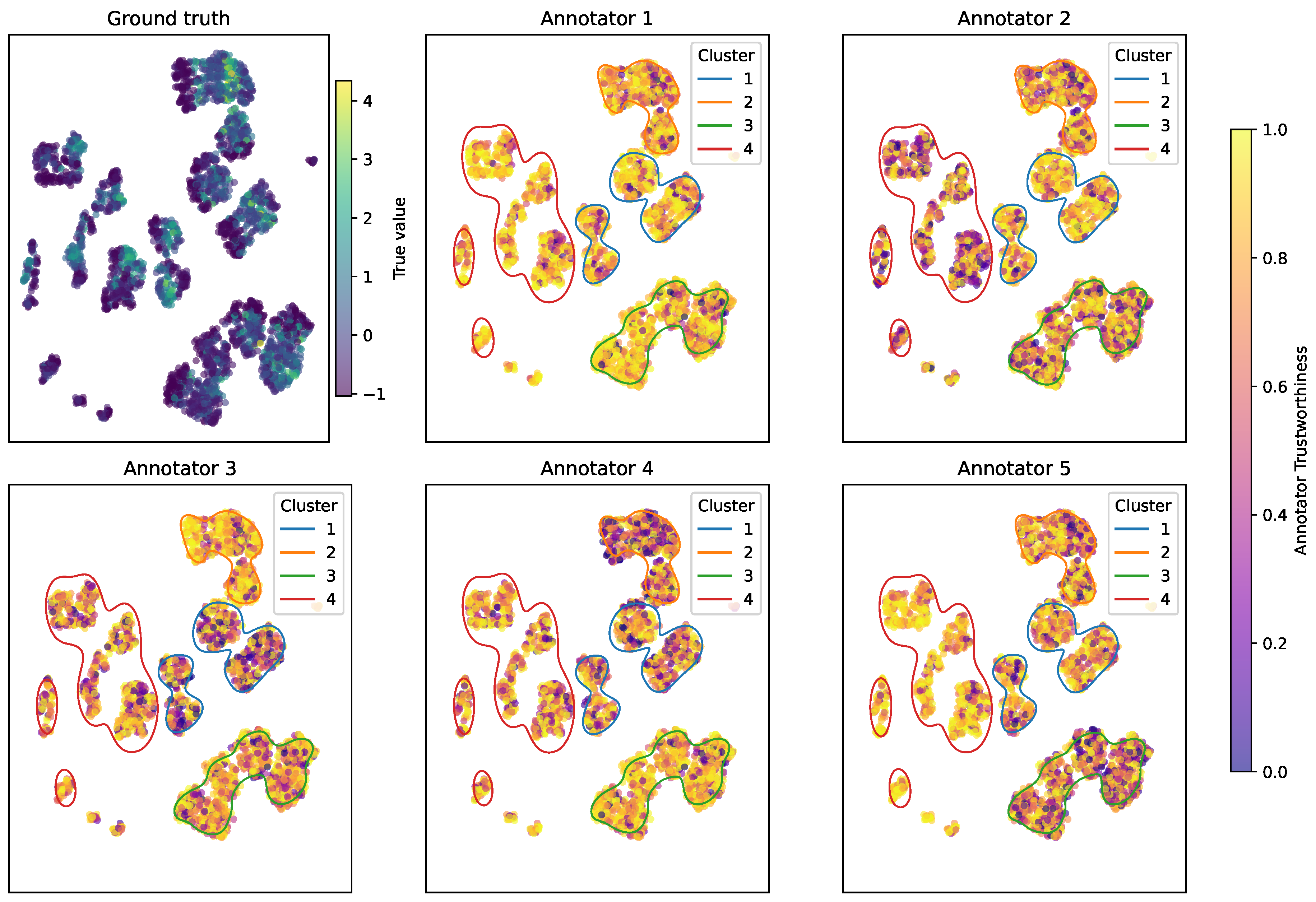
Figure 12.
Average annotator trustworthiness across all evaluated semi-synthetics datasets. Left: Average empirical scores measuring the agreement between each annotator’s labels and the corresponding ground truth. Right: Average MAR-CCGP trustworthiness scores estimated for each annotator. A strong correspondence is evident between the two metrics, with a Pearson correlation of 0.853.
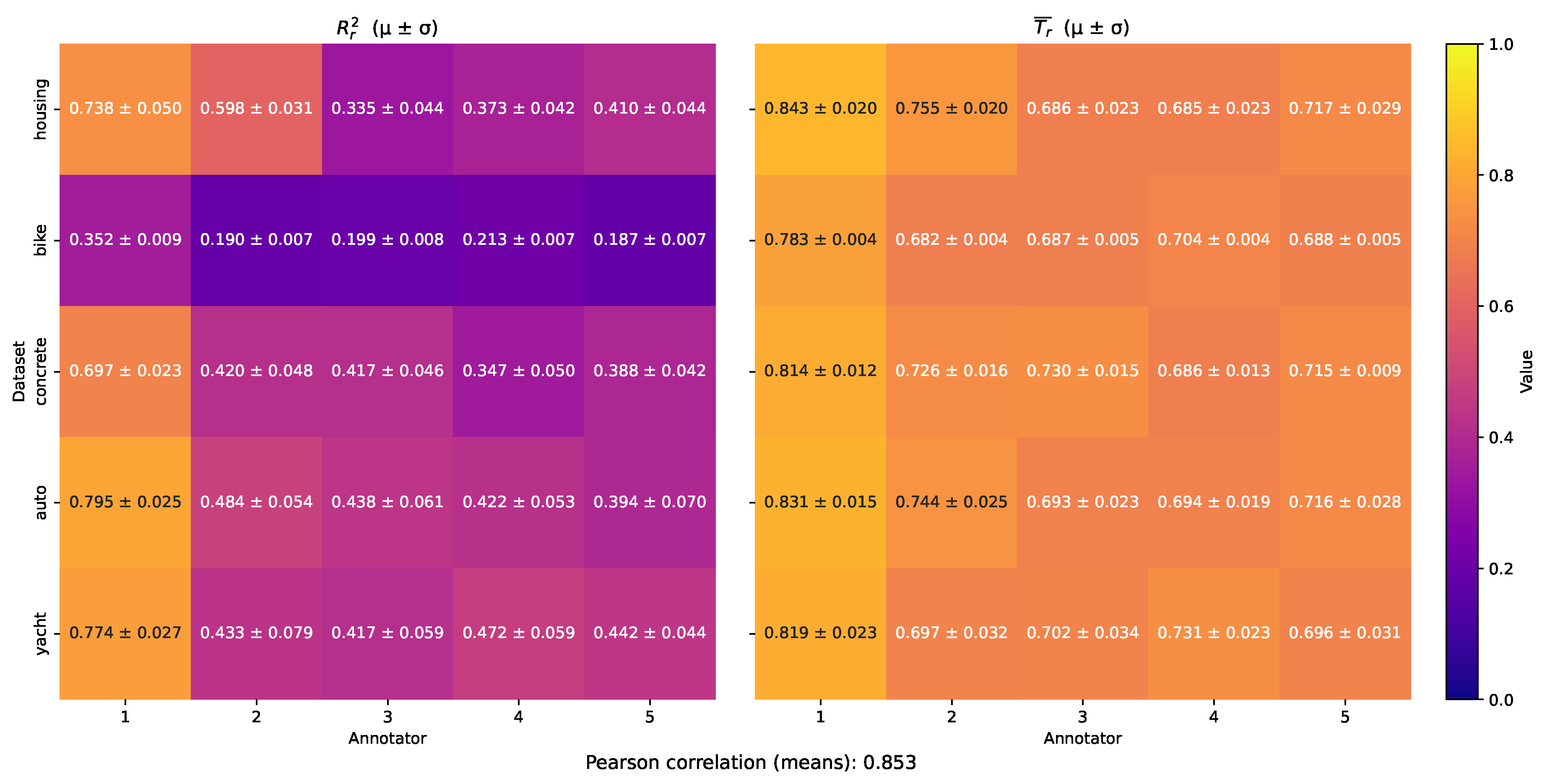
Figure 13.
Estimated ground truth sweetness (solid brown line) and its associated predictive uncertainty (shaded region), compared against individual annotators’ sweetness scores for the LUKER-CACAO dataset. Samples are sorted by the model’s estimated mean sweetness value.
Figure 13.
Estimated ground truth sweetness (solid brown line) and its associated predictive uncertainty (shaded region), compared against individual annotators’ sweetness scores for the LUKER-CACAO dataset. Samples are sorted by the model’s estimated mean sweetness value.

Figure 14.
Bipartite graph representing the Pearson correlations between each physicochemical feature (left, blue nodes) and the estimated trustworthiness of each annotator (right, pink nodes). Edge color encodes the magnitude and sign of the correlation, with red indicating positive and blue indicating negative correlations.
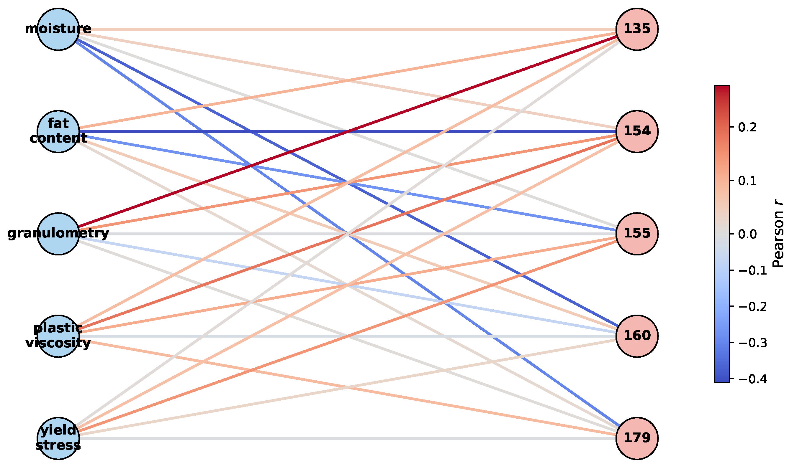
Figure 15.
UMAP projections for the LUKER-CACAO dataset showing the estimated ground truth and annotator-specific trustworthiness for the sweetness attribute. Top left: Ground truth estimated by MAR-CCGP. Remaining panels: Trustworthiness scores inferred for each annotator (135, 154, 155, 160, and 179). Marker shapes denote the product type, allowing comparison of trust patterns across different product categories.
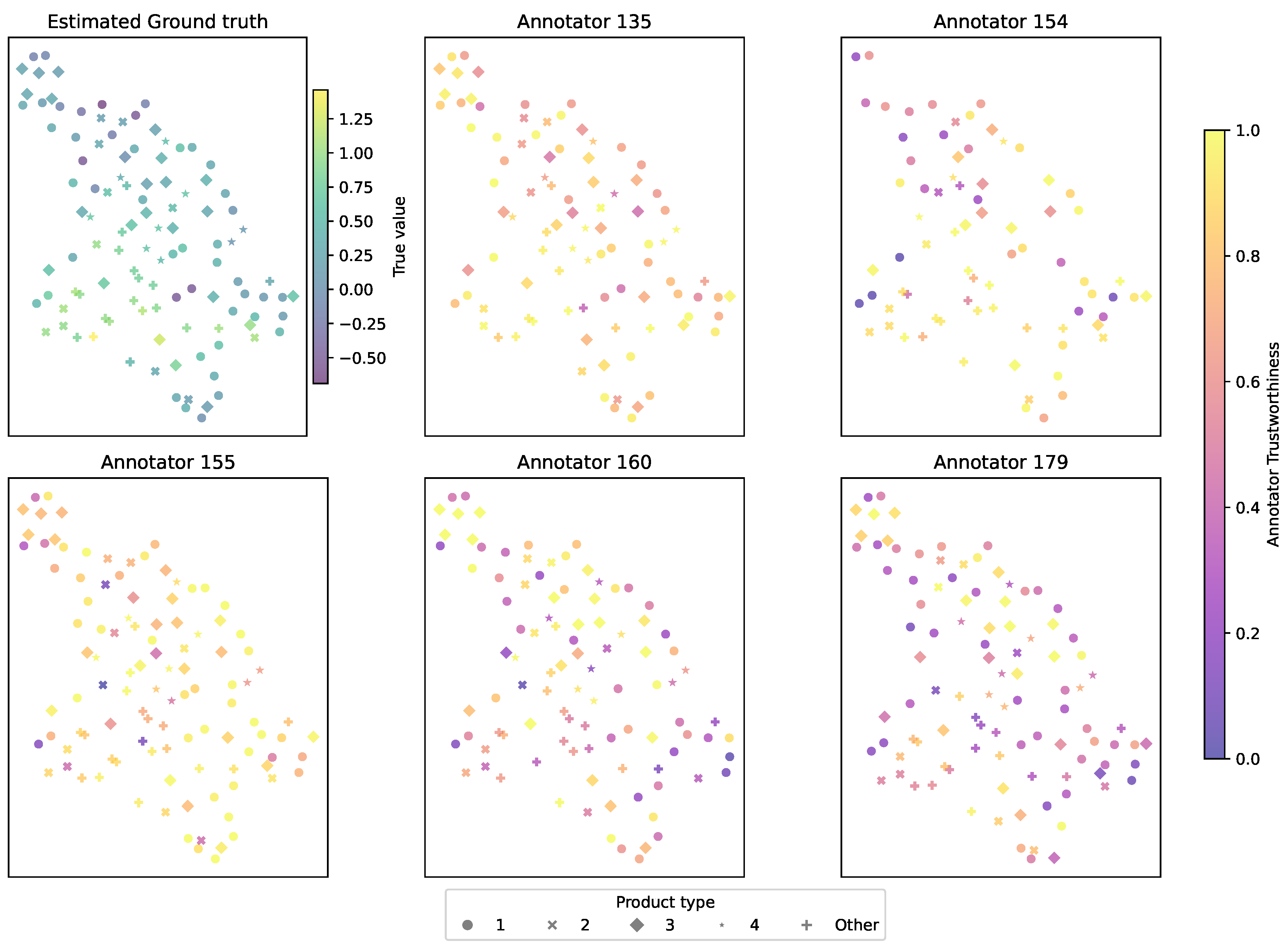
Figure 16.
Summary heatmap of average annotator trustworthiness () across all sensory variables and annotators, showing per-attribute trustworthiness profiles derived by MAR-CCGP. Values represent the mean trust scores with their corresponding standard deviations, and color indicates the relative trust level.

Table 1.
Standard analytical methods used for each selected physicochemical and sensory variables.
| Variable | Analytical method |
|---|---|
| Fat Content | AOAC Official Method 963.15 [38] |
| Moisture | AOAC Official Method 931.04 [39] |
| Granulometry | ISO 13320:2020 [40] |
| Plastic Viscosity | IOCCC Method 46 [41] |
| Yield Stress | IOCCC Method 46 [41] |
| Sensory Attributes | NTC 3932 [42] |
Table 2.
Label completeness per annotator and sensory variable in the cacao-based product database. Each value represents the percentage of non-missing labels relative to the total number of retained samples for that attribute.
Table 2.
Label completeness per annotator and sensory variable in the cacao-based product database. Each value represents the percentage of non-missing labels relative to the total number of retained samples for that attribute.
| Annotator | Acidity | Bitterness | Aroma | Astringency | Sweetness | Hardness | Global impression | Melting speed |
|---|---|---|---|---|---|---|---|---|
| 135 | 86.1 | 86.1 | 85.6 | 90.2 | 85.5 | 85.5 | 85.5 | 85.5 |
| 154 | 70.8 | 70.8 | 69.4 | 68.9 | 69.1 | 69.1 | 69.1 | 69.1 |
| 155 | 95.8 | 95.8 | 97.3 | 95.1 | 97.3 | 97.3 | 97.3 | 97.3 |
| 160 | 88.9 | 88.9 | 90.1 | 90.2 | 90.0 | 90.0 | 90.0 | 90.0 |
| 179 | 88.9 | 88.9 | 91.9 | 91.8 | 91.8 | 91.8 | 91.8 | 91.8 |
| Available samples | 72 | 72 | 111 | 61 | 110 | 110 | 110 | 110 |
Table 3.
Completeness of input features and number of samples per task for the Cacao-based product database. Completeness is measured as the percentage of non-missing values for each physicochemical variable in the final dataset associated with each sensory attribute.
Table 3.
Completeness of input features and number of samples per task for the Cacao-based product database. Completeness is measured as the percentage of non-missing values for each physicochemical variable in the final dataset associated with each sensory attribute.
| Physico- chemical/Sensory | Acidity | Bitterness | Aroma | Astringency | Sweetness | Hardness | Global impression | Melting speed |
|---|---|---|---|---|---|---|---|---|
| Moisture | 98.6 | 98.6 | 99.1 | 98.4 | 99.1 | 99.1 | 99.1 | 99.1 |
| Fat Content | 95.8 | 95.8 | 97.3 | 95.1 | 97.3 | 97.3 | 97.3 | 97.3 |
| Granulometry | 88.9 | 88.9 | 91.9 | 86.9 | 92.7 | 92.7 | 92.7 | 92.7 |
| Plastic viscosity | 100.0 | 100.0 | 100.0 | 100.0 | 100.0 | 100.0 | 100.0 | 100.0 |
| Yield stress | 97.2 | 97.2 | 98.2 | 96.7 | 98.2 | 98.2 | 98.2 | 98.2 |
| Available samples | 72 | 72 | 111 | 61 | 110 | 110 | 110 | 110 |
Table 4.
Summary of benchmark regression datasets from the UCI repository used for simulating semi-synthetic multi-annotator annotations.
Table 4.
Summary of benchmark regression datasets from the UCI repository used for simulating semi-synthetic multi-annotator annotations.
| Dataset | # Samples | # Features |
|---|---|---|
| Bike Sharing | 17379 | 11 |
| Concrete Strength | 1030 | 8 |
| Boston Housing | 501 | 13 |
| Auto MPG | 392 | 7 |
| Yacht Hydrodynamics | 308 | 6 |
Table 6.
Global regression measures for the semi-synthetics datasets. Average ± standard deviation across 15 folds for each method and dataset are depicted.
Table 6.
Global regression measures for the semi-synthetics datasets. Average ± standard deviation across 15 folds for each method and dataset are depicted.
| Dataset | Method | MSE | MAE | MAPE | |
|---|---|---|---|---|---|
| BostonHousing | GPR-AVG | ||||
| GPR-GT | |||||
| LKAAR | |||||
| MAR-CCGP | |||||
| BikeSharing | GPR-AVG | ||||
| GPR-GT | |||||
| LKAAR | |||||
| MAR-CCGP | |||||
| ConcreteStrength | GPR-AVG | ||||
| GPR-GT | |||||
| LKAAR | |||||
| MAR-CCGP | |||||
| Auto MPG | GPR-AVG | ||||
| GPR-GT | |||||
| LKAAR | |||||
| MAR-CCGP | |||||
| YachtHydrodynamics | GPR-AVG | ||||
| GPR-GT | |||||
| LKAAR | |||||
| MAR-CCGP |
Table 7.
Annotator Trustworthiness (Mean ± Std) for each variable and product (highest mean value per row is in bold).
Table 7.
Annotator Trustworthiness (Mean ± Std) for each variable and product (highest mean value per row is in bold).
| Variable | Product Type | 135 | 154 | 155 | 160 | 179 |
|---|---|---|---|---|---|---|
| acidity | 1 | 0.63 ± 0.09 | 0.79 ± 0.06 | 0.74 ± 0.08 | 0.78 ± 0.07 | 0.53 ± 0.08 |
| 2 | 0.82 ± 0.10 | 0.89 ± 0.08 | 0.88 ± 0.08 | 0.90 ± 0.05 | 0.79 ± 0.08 | |
| 3 | 0.85 ± 0.14 | 0.79 ± 0.10 | 0.88 ± 0.11 | 0.74 ± 0.07 | 0.83 ± 0.14 | |
| 4 | 0.70 ± 0.20 | 0.86 ± 0.09 | 0.72 ± 0.17 | 0.83 ± 0.07 | 0.53 ± 0.12 | |
| General | 0.80 ± 0.19 | 0.88 ± 0.10 | 0.84 ± 0.18 | 0.88 ± 0.09 | 0.69 ± 0.20 | |
| bitterness | 1 | 0.70 ± 0.06 | 0.68 ± 0.06 | 0.67 ± 0.08 | 0.84 ± 0.06 | 0.83 ± 0.04 |
| 2 | 0.59 ± 0.19 | 0.47 ± 0.24 | 0.56 ± 0.18 | 0.48 ± 0.24 | 0.67 ± 0.11 | |
| 3 | 0.93 ± 0.04 | 0.99 ± 0.01 | 0.85 ± 0.12 | 0.52 ± 0.18 | 0.53 ± 0.27 | |
| 4 | 0.73 ± 0.14 | 0.79 ± 0.19 | 0.71 ± 0.19 | 0.71 ± 0.13 | 0.90 ± 0.06 | |
| General | 0.75 ± 0.19 | 0.77 ± 0.27 | 0.70 ± 0.23 | 0.62 ± 0.25 | 0.66 ± 0.27 | |
| aroma | 1 | 0.65 ± 0.05 | 0.60 ± 0.05 | 0.92 ± 0.04 | 0.69 ± 0.07 | 0.84 ± 0.09 |
| 2 | 0.63 ± 0.06 | 0.63 ± 0.12 | 0.79 ± 0.13 | 0.65 ± 0.23 | 0.84 ± 0.18 | |
| 3 | 0.71 ± 0.06 | 0.51 ± 0.12 | 0.79 ± 0.06 | 0.52 ± 0.14 | 0.84 ± 0.12 | |
| 4 | 0.83 ± 0.14 | 0.72 ± 0.01 | 0.90 ± 0.17 | 0.29 ± 0.12 | 0.73 ± 0.26 | |
| General | 0.73 ± 0.17 | 0.66 ± 0.13 | 0.86 ± 0.14 | 0.59 ± 0.25 | 0.86 ± 0.18 | |
| astringency | 1 | 0.65 ± 0.09 | 0.70 ± 0.08 | 0.72 ± 0.06 | 0.80 ± 0.06 | 0.84 ± 0.05 |
| 2 | 0.62 ± 0.09 | 0.56 ± 0.23 | 0.70 ± 0.24 | 0.46 ± 0.17 | 0.85 ± 0.17 | |
| 3 | 0.52 ± 0.11 | 0.46 ± 0.11 | 0.90 ± 0.06 | 0.83 ± 0.10 | 0.97 ± 0.02 | |
| 4 | 0.71 ± 0.12 | 0.46 ± 0.14 | 0.81 ± 0.15 | 0.79 ± 0.10 | 0.63 ± 0.20 | |
| General | 0.65 ± 0.15 | 0.53 ± 0.16 | 0.77 ± 0.18 | 0.73 ± 0.20 | 0.76 ± 0.28 | |
| sweetness | 1 | 0.80 ± 0.05 | 0.55 ± 0.11 | 0.82 ± 0.06 | 0.52 ± 0.07 | 0.43 ± 0.06 |
| 2 | 0.72 ± 0.11 | 0.61 ± 0.15 | 0.52 ± 0.18 | 0.70 ± 0.11 | 0.77 ± 0.15 | |
| 3 | 0.73 ± 0.08 | 0.79 ± 0.12 | 0.74 ± 0.06 | 0.93 ± 0.07 | 0.84 ± 0.08 | |
| 4 | 0.84 ± 0.13 | 0.88 ± 0.05 | 0.80 ± 0.13 | 0.62 ± 0.21 | 0.52 ± 0.11 | |
| General | 0.76 ± 0.17 | 0.80 ± 0.16 | 0.72 ± 0.19 | 0.69 ± 0.19 | 0.66 ± 0.21 | |
| hardness | 1 | 0.61 ± 0.08 | 0.87 ± 0.08 | 0.87 ± 0.06 | 0.73 ± 0.10 | 0.88 ± 0.05 |
| 2 | 0.62 ± 0.09 | 0.85 ± 0.12 | 0.84 ± 0.16 | 0.77 ± 0.12 | 0.89 ± 0.14 | |
| 3 | 0.67 ± 0.12 | 0.77 ± 0.26 | 0.89 ± 0.07 | 0.88 ± 0.09 | 0.90 ± 0.07 | |
| 4 | 0.70 ± 0.10 | 0.87 ± 0.09 | 0.94 ± 0.08 | 0.73 ± 0.12 | 0.86 ± 0.10 | |
| General | 0.67 ± 0.21 | 0.59 ± 0.34 | 0.84 ± 0.21 | 0.70 ± 0.26 | 0.82 ± 0.22 | |
| global impression | 1 | 0.69 ± 0.06 | 0.85 ± 0.08 | 0.91 ± 0.06 | 0.64 ± 0.06 | 0.77 ± 0.09 |
| 2 | 0.55 ± 0.07 | 0.75 ± 0.20 | 0.96 ± 0.07 | 0.55 ± 0.11 | 0.83 ± 0.16 | |
| 3 | 0.65 ± 0.08 | 0.81 ± 0.17 | 0.88 ± 0.11 | 0.52 ± 0.10 | 0.86 ± 0.11 | |
| 4 | 0.39 ± 0.11 | 0.96 ± 0.08 | 0.98 ± 0.02 | 0.42 ± 0.20 | 0.50 ± 0.28 | |
| General | 0.57 ± 0.21 | 0.82 ± 0.16 | 0.91 ± 0.18 | 0.58 ± 0.15 | 0.78 ± 0.25 | |
| melting speed | 1 | 0.77 ± 0.05 | 0.97 ± 0.05 | 0.80 ± 0.05 | 0.75 ± 0.06 | 0.73 ± 0.04 |
| 2 | 0.88 ± 0.07 | 0.89 ± 0.17 | 0.89 ± 0.04 | 0.61 ± 0.17 | 0.77 ± 0.02 | |
| 3 | 0.77 ± 0.07 | 0.98 ± 0.03 | 0.75 ± 0.08 | 0.72 ± 0.09 | 0.78 ± 0.03 | |
| 4 | 0.90 ± 0.08 | 1.00 ± 0.01 | 0.94 ± 0.06 | 0.64 ± 0.10 | 0.72 ± 0.03 | |
| General | 0.77 ± 0.19 | 0.82 ± 0.27 | 0.81 ± 0.11 | 0.68 ± 0.21 | 0.77 ± 0.06 |
Disclaimer/Publisher’s Note: The statements, opinions and data contained in all publications are solely those of the individual author(s) and contributor(s) and not of MDPI and/or the editor(s). MDPI and/or the editor(s) disclaim responsibility for any injury to people or property resulting from any ideas, methods, instructions or products referred to in the content. |
© 2025 by the authors. Licensee MDPI, Basel, Switzerland. This article is an open access article distributed under the terms and conditions of the Creative Commons Attribution (CC BY) license (http://creativecommons.org/licenses/by/4.0/).
Copyright: This open access article is published under a Creative Commons CC BY 4.0 license, which permit the free download, distribution, and reuse, provided that the author and preprint are cited in any reuse.


