Submitted:
01 July 2025
Posted:
03 July 2025
You are already at the latest version
Abstract
This paper focuses on the specific mechanism of manufacturing agglomeration on the economic circulations, and makes a theoretical analysis and explanation by constructing a spatial equilibrium model of new economic geography from three perspectives: domestic circulation, international circulation and “dual circulation” coordination. The results show that: at present, manufacturing agglomeration mainly contributes to the domestic circulation, but has no significant effect on international circulation. The results of further analysis show that the promoting effect of manufacturing agglomeration on domestic circulation will change due to the differentiation of regional factor endowments, while the overall effect of manufacturing agglomeration on international circulation is not significant, which may be due to the differences in regional trade costs and the elasticity of returns to scale of manufacturing industry.
Keywords:
manufacturing agglomeration
; economic circulation
; TOPSIS entropy weight method
; spatial equilibrium model
1. Introduction
China’s rapid industrialization has concentrated manufacturing in coastal regions, amplifying regional disparities while integrating into global value chains. The “dual circulation” strategy (prioritizing domestic demand while upgrading international competitiveness) raises a key question: How does manufacturing agglomeration shape economic circulation? The spatial distribution and upgrading of manufacturing industry have attracted wide attention. Manufacturing agglomeration is an important factor in shaping economic geography. Through spatial proximity, the economic effects brought by externalities have promoted the rapid expansion of cities and formed the problem of unbalanced development between regions (Fujita et al., 2001). Most of the existing literature focuses on the externalities brought by agglomeration when discussing the relationship between manufacturing agglomeration and economic growth, scholars believe that agglomeration is promoting the development of innovation factors (Ying et al., 2021; Gordon and McCann, 2005), the efficiency of inter-regional flow of production factors (Yuan et al., 2023; Otsuka, 2020), and urbanization and industrialization (Liang et al., 2019; Hua et al., 2019), and other aspect. This kind of research regards increasing returns to scale as local production externalities, and most of the analytical frameworks are based on the assumption of perfect competition. It has produced rich and detailed literature to illustrate the key role of manufacturing agglomeration in the formation and development of China’s modern industrialization in the past few decades, and has promoted the transformation and upgrading of industries in various fields in China.
At present, most of the literature research on economic circulation focuses on the concept and connotation interpretation, and index system construction of its economic characteristics. The economic circulation theory includes economic modernization theory, reproduction theory and others (Ingebrigtsen and Jakobsen, 2007). Based on this, some Chinese scholars have carried out the exploration of China’s “dual circulation” economic development model, such as Javed et al. (2021) and Huang et al. (2022). And the upgrading of the manufacturing industry has played an important role in this economic circulation (Guo and Tian, 2022). By deepening the supply-side structural reform, the industrial layout and structural adjustment have been driven to achieve a smooth economic circulation (Xie et al., 2020). In reality, there are some problems in the construction of China’s “dual circulation” pattern, such as insufficient domestic circulation, unbalanced domestic and international dual circulation, and unsmooth circulation of production factors. At the same time, the conditions and space of China’s domestic industrial chain and supply chain have also undergone profound changes. Therefore, how to combine the reality and advantages of China’s economic development to improve the economic circulation is becoming more and more important. Nowadays, the world economic development presents the dual characteristics of economic globalization and industrial agglomeration, China’s development strategic objectives also require the realization of the coordination and complementarity of the two circulations of domestic and international. There are limitations in the explanatory power of single use of international trade theory or regional development theory.
Compared with previous studies, the marginal contribution of this paper lies in: First, under a unified framework of spatial economics analysis, this paper discusses the theoretical path of manufacturing agglomeration affecting economic circulation, and provides an analysis perspective of agglomeration and economic circulation under the premise of increasing returns to scale and monopolistic competition. Second, based on the theory of economic circulation, this paper constructs the performance index of “dual circulation” pattern, and empirically analyzes the role of manufacturing agglomeration in “dual circulation” pattern. Third, based on the differences at the regional and industry levels, this paper discusses the potential mechanism of the influence of manufacturing agglomeration on “dual circulation” pattern, which enriches the empirical facts and theoretical explanations of the relationship between agglomeration and economic circulation.
2. Modelling Framework
2.1. Three-Region Spatial Equilibrium Model
Considering a spatial equilibrium model under the new economic geography framework, it is assumed that there are three regions 0, 1 and 2 in the economy, of which region 1 and region 2 are two regions in China, and region 0 represents the rest of the world. Each region consists of two sectors: manufacturing sector M producing manufactured goods and non-manufacturing sector A producing other goods. Sector A is completely competitive, using the technology of constant returns to scale to produce a single homogeneous product; Sector M is monopolistic competition, using the technology of increasing returns to scale to produce differentiated products. The production of the two sectors needs to invest two factors: labor (L) and capital (K). In order to simplify the analysis, the share of capital in each region is endogenously determined by its own rate of return θ. The labor force in sector A cannot flow, and the labor force in sector M cannot flow across countries, but it can flow between Region 1 and Region 2 after long-term equilibrium1, and it is assumed that the total labor force of sector M in Region 1 and Region 2 is the unit, and the share of Region 1 is λ, then the share of Region 2 is 1-λ. In order to exclude the influence of Heckscher-Ohlin comparative advantage, it is assumed that the factor endowments, preferences and technologies of the three regions are exactly the same. For the manufacturing sector in Region 1, the larger the share λ is, the more labor force engaged in manufacturing absorbed locally. Because the total domestic labor force is certain, and there is no difference in other factor endowments and technologies between Region 1 and Region 2, when , the manufacturing production scale of Region 1 will be greater than that of Region 2, that is, the degree of manufacturing agglomeration will be higher. Therefore, in the following analysis, the labor share λ of the manufacturing sector M is used to indicate the degree of manufacturing agglomeration.
Assumed that the consumer utility function is in the following Cobb-Douglas form:
Among them, μ represents the expenditure share of manufacturing product M. For the set M composed of different product consumptions in continuous space, it can be expressed by the constant elasticity of substitution function:
In the above formula, n represents the range of products that consumers can consume, represents the consumption of each manufacturing product, and parameter ρ represents the degree of consumer preference for the diversity of manufacturing products. The greater the parameter ρ is, the stronger the substitutability of the product have. Given that the income is Y, PM and PA represent the price of manufacturing products and the price of non-manufacturing products, respectively. Since sector A is perfectly competitive and PA has the same value in each region, the utility maximization problem of consumers under budget constraints can be transformed into the problem of selecting each to minimize the M expenditure. According to the first-order condition, the Hicks demand function of consumers for each manufacturing product can be expressed as:
Integral calculation of each product expenditure:
Then, the price index PM is the lowest expenditure for the consumption of one unit of manufacturing product M:
Furthermore, the Marshall demand can be calculated:
Among them, represents the elasticity of substitution of any two products. According to the value range of ρ, . With the increase of product variety, the price index PM will decrease, and the smaller the substitution elasticity σ, the greater the decrease of the price index.
Due to the increasing returns to scale, the manufacturing industry in each region will tend to specialize in the production of specific products, forming a division of labor to generate trade. It is assumed that there is no cost in the local transportation of manufacturing products, and the cost in cross-regional transportation is measured in the form of Samuelson’s “iceberg cost”. Taking the cross-regional trade between Region 1 and Region 2 as an example, when a unit of product is transported from Region 1 to Region 2, only part of good can reach. Therefore, Region 1 needs to produce unit product to ensure that 1 unit product can reach Region 2. Accordingly, if the price of the product in Region 1 is , the price of consuming this product in Region 2 is . Obviously, due to the different products produced in each region, the price index of its manufacturing products is also different. The price index of manufacturing products in region s is recorded as Gs to represent this difference:
Substituting Equation (8) into Equation (7), the demand for manufacturing products produced by region t in region s can be obtained. By summing up, the total demand faced by the product in region t can be obtained:
Next, we consider the production behavior of each department. Sector A inputs only labor and output a single homogeneous product. Therefore, the product price and labor remuneration are equal in the equilibrium, which is no longer pointed out separately in the subsequent analysis. The representative enterprise production function of M sector can be expressed as:
Among them, F is the fixed cost, c is the marginal cost, and β represents the capital input share of enterprise production. The larger the β is, the higher the capital intensity of the manufacturing industry is.
Due to the existence of economies of scale, for a new entrant, the production of new products is more advantageous than the production of existing products, so it is assumed that the type of product and the number of enterprises is correspondence. The manufacturer’s profit function of Region s can be expressed as:
Among them, w and r respectively represent the remuneration of labor and capital, that is, workers’ wages and return of capital.
Under the optimal factor input level, the pricing of manufacturing products produced by enterprises in Region s according to the principle of profit maximization should be:
2.2. Domestic Economic Circulation Equilibrium
First of all, we focus on the market equilibrium of domestic circulation. The number of manufacturing enterprises in Region s under market clearing conditions, that is, the number of types of manufacturing products, is endogenously determined by locally owned production factors. Since the production equations of all manufacturing sectors are symmetrical, taking Region 1 as an example, the equilibrium is:
The equilibrium output under the condition of zero profit is:
The ratio of factor return in equilibrium can be expressed as:
If the capital in Region 1 is held on average by workers in the M sector, then the total income of each worker can be further expressed as:
It can be seen that the income of workers in Region 1 is related to the capital intensity of the overall economy (here refers to the domestic economy composed of Region 1 and Region 2), the degree of factor agglomeration in Region 1 and the relative supply of factors, and is proportional to the labor remuneration of workers. The domestic circulation is based on meeting domestic demand as the starting point and foothold. China has a super-large market, not only has the world’s largest population size, but more importantly, has the world’s largest middle-income population, how to improve residents’ income, thereby stimulating domestic demand growth, and improving the endogenous power and reliability of the domestic circulation is an important issue of concern in this paper. By combining Equations (12) - (15), the labor remuneration of Region 1 in equilibrium can be obtained, that is, the worker’s wage is2:
From the short-term perspective of domestic circular market equilibrium, due to the inability of workers to flow across regions, only capital flows freely between regions to seek higher returns on capital. At the same time, taking into account the existence of trade barriers, investment restrictions, etc., the speed of international capital flows is often significantly slower than the speed of capital flows between domestic regions. It may be assumed that the share of foreign capital is exogenous, and wage income is affected by the combined effects of regional manufacturing labor share λ (manufacturing agglomeration), regional capital share θ, production factor ratio and regional price index. When , the return of capital in the two regions is the same, and the capital stops flowing. According to Equation (15), the nominal wages of Region 1 and Region 2 satisfy at this time.
It can be seen that the allocation of production factors such as capital and labor between regions will further affect the income gap between regions. Due to the complexity of the wage equation, the direct relationship between λ, θ1 and w1 cannot be intuitively seen in the equilibrium solution results, which can be further decomposed by the total differential of equation (17). When the difficulty of substitution between products is higher than the share of capital input in the production process (), the positive effect of manufacturing agglomeration on income is more obvious. The economic implication behind this is that when the competitive characteristics in the monopolistic competition market are more obvious, regions with lower capital intensity can increase the labor income of workers by expanding the production of the manufacturing sector and forming an agglomeration effect, thus stabilizing the domestic market economy circulation driven by domestic demand.
Next, consider the economic circulation between domestic regions. If the definition of Region 1 and 2 is at the provincial level, the inter-regional circulation is the inter-provincial circulation. In order to highlight the economic circulation characteristics between different provinces, the relevant parameters of Region 0 are further externalized here, and capital K and capital return rate r are unitized. Then in equilibrium, Regions 1 and 2 satisfy the following equality:
After the total differential of the total income, we can get3:
Let , according to the value ranges of , . When , at this time, the inter- provincial trade cost is the lowest, the degree of regional integration is the highest, and the inter-provincial circulation is unimpeded; when , at this time, the inter-regional trade costs are extremely high, inter-provincial trade does not occur, and the inter-provincial circulation will be interrupted. Z is brought into Equation (24) and Equation (25), which can be simplified as follow:
When Z = 0, there is no transportation cost in interregional trade, at this time, which indicates that when the degree of regional integration reaches the highest, that is, there is no interregional gap, the share of manufacturing in each region will no longer affect income. In fact, Region 1 and Region 2 can be regarded as a whole in this situation. In most cases, Z is arbitrary between (0,1), and the value of depends on the relationship between the elasticity of substitution ρ and the manufacturing products demand μ. When , the higher the local manufacturing share (degree of agglomeration), the higher the wage income of workers. Based on the above analysis, some very meaningful conclusions can be drawn. With the reduction of inter-regional trade costs, the degree of domestic integration has gradually deepened, inter-provincial trade barriers have been broken, and the domestic income gap will be reduced. On the other hand, when the consumption of industrial manufactured goods within the region is high, the agglomeration of manufacturing industry can increase the local wage income, and then transform it into more consumption of industrial manufactured goods, and further improve the local wage income, and play the circular causal effect of agglomeration.
2.3. International Economic Circulation Equilibrium
In this part of the analysis, we will pay more attention to the equilibrium analysis of the domestic market’s participation in the international circulation. Referring to Deng’s (2009) approach, here, Region 1 and Region 2 are regarded as a whole, that is, the whole domestic market (represented by Region C), and the regional ROW (rest of the world) represents the international market. Correspondingly, the capital share of the domestic market is denoted as θ, and the capital share of the international market can be expressed as 1-θ. If the domestic labor share is still recorded as λ, the labor share of the international market can be expressed as 1-λ, and according to the reality, let , that is, China has a relatively larger labor market and consumer market. The transaction cost is still the “iceberg cost” mode, transporting one unit of product to another area, only unit arrives, and the “melting” part is the transaction cost.
The condition of capital short-term equilibrium is , that is, after the return on capital at home and abroad is equal, capital stops flowing. In equilibrium:
Where , and .
Similar to the domestic market equilibrium, it is difficult to obtain an intuitive relationship between λ and θ from the equilibrium, but some conclusions can still be obtained through comparative analysis under the premise assumption. When , at this time, that is, the degree of capital intensity will exceed the degree of agglomeration of manufacturing labor, and vice versa. The results show that in the process of China’s participation in the international circulation, if the cost of international trade is low, it will attract capital from all regions of the world to invest domestically, thus improving the current industrial structure dominated by labor-intensive industries and developing capital-intensive industries. For the Chinese mainland market with large regional development differences, it is a reasonable choice for the eastern region to use the excess product demand brought by manufacturing agglomeration for large-scale production to exert the local market effect for international trade (Krugman, 1980). The central and western regions that lack manufacturing agglomeration and FDI should pay more attention to the internal market demand of the region and the demand of other regions in the country. It may be a feasible choice to gradually cultivate the local market effect of related industries.
3. Economic Circulation Index Design
3.1. Dual Circulation Pattern
The specific description of the dual circulation is shown in Table 1. This paper draws on the research results of Li et al. (2022). Firstly, the TOPSIS entropy weight method is used to measure the development level of the two indicators of the domestic and international circulations in each region, and then the coupling coordination degree model is constructed to calculate the coupling coordination degree of the economic dual circulation to represent the performance indicators of the new development pattern of the dual circulation in each region.
The steps of the TOPSIS entropy weight method to calculate the indicators of the National Circulation and the International Circulation are as follows:
- (1)
- Standardized processing of the initial index data
- (2)
- Calculate entropy and weight
- (3)
- Construct a weighting matrix and determine the optimal solution and the worst solution
- (4)
- Calculate the Euclidean distance between the optimal solution and the worst solution
- (5)
- Calculate relative proximity
- (6)
- Calculate the coupling coordination degree
Among them, D represents the coupling coordination degree value of the economic internal circulation system and the economic external circulation system, the value range is between 0 and 1, α and β are the undetermined weight coefficients, and α + β = 1. The values of α and β need to consider the importance of the two economic circulations, after referring to the foreign trade dependence index of the world’s major economies, this paper believes that the domestic circulation weight of China’s dual circulation coordinated development of the economy should not be less than 0.5.
3.2. “Dual Circulation” Index Measurement Results
Table 2 shows Beijing, Shanghai, and Tianjin leading China's 2020 provincial dual-circulation performance, with balanced domestic-international circulation scores above the “on the verge of imbalance” threshold. However, over half of provinces exhibit moderate to severe imbalances, reflecting underdeveloped domestic markets, overreliance on low-value global chains, and fragile economic transitions. Most regions struggle to coordinate internal demand expansion with external competitiveness.
4. Analysis of Empirical Results
The analysis reveals that manufacturing agglomeration exhibits dual effects on China's dual circulation paradigm. Under specific conditions, it elevates household income levels and stimulates demand through cyclical agglomeration effects, thereby enhancing domestic circulation reliability. Simultaneously, it amplifies export competitiveness via local market effects, facilitating international circulation. However, structural challenges emerge from China's unique institutional context: interprovincial non-market competition under fiscal decentralization, coupled with capital-technology flow uncertainties in external circulation, complicate agglomeration outcomes. This study employs an econometric model to investigate how manufacturing spatial concentration interacts with these institutional and structural factors in shaping the dual circulation dynamics, particularly given China's vast market scale and heterogeneous regional development objectives.
Among them, i represents the region, t represents the year, is the explained variable, this paper analyzed the results from three aspects: the domestic circulation, the international circulation and the dual circulation coupling coordination degree. The core explanatory variable is the level of manufacturing agglomeration in each region, which is expressed by the location entropy of the number of manufacturing employees in each region. The control variables at the provincial level include per capita GDP, industrial structure, urbanization rate, fiscal expenditure, road accessibility and R & D intensity. Considering that the explained variables are composite indicators, the selection of control variables should avoid the use of relevant data included in the construction of dual circulation indicators. Therefore, nighttime light data are selected as the proxy variable of per capita GDP to control the differences in economic development levels among provinces. Nighttime light data record daily economic activities and energy consumption, and can also reflect some information that is difficult to be transmitted by traditional GDP data (Gibson et al., 2020).
4.1. Benchmark Regression
Table 3 presents OLS regression results showing manufacturing agglomeration's positive impact on dual circulation, with coefficients increasing as domestic circulation weights rise from 0.5 to 0.9. For instance, a domestic weight of 0.7 yields a significant 0.0201 coefficient, indicating a 2.01% boost to dual circulation performance when agglomeration doubles. While domestic circulation shows strong significance (coefficient = 0.0177, p<0.01), international circulation effects are statistically insignificant (0.0025), highlighting agglomeration's primary role in enhancing domestic economic flows.
The study finds manufacturing agglomeration strengthens domestic economic circulation through production-consumption-distribution linkages, with expanding agglomeration scales (from special zones to national markets) enhancing resource allocation, knowledge spillovers, and inter-regional specialization. This reduces production/transaction costs while boosting innovation, labor productivity, and income—stabilizing domestic demand-driven growth. Unified markets further mitigate negative agglomeration externalities by weakening regional boundaries and promoting balanced factor distribution. For the foreign circulation, China's international circulation faces heightened requirements and risk management challenges. The home market effect suggests that under monopolistic competition and increasing returns to scale, large domestic markets foster net exports (Davis and Weisteins, 2003), yet manufacturing agglomeration's limited impact on international circulation may stem from: (1) lower inter-provincial versus international trade costs, which prioritize domestic market effects, and (2) insufficient returns to scale in manufacturing, as industries with weaker scale economies tend toward self-sufficiency (Holmes and Stevens, 2005). These factors warrant further analysis.
4.2. Robustness Test
To address potential endogeneity between manufacturing agglomeration (measured by employment location quotient) and dual-circulation performance, this study employs instrumental variables (IV) using topographic relief and river density—natural factors that hinder agglomeration due to geographic isolation but remain exogenous to economic conditions. The 2SLS results (Table 4) confirm robust first-stage relevance (F > 10) and yield consistent findings: manufacturing agglomeration significantly enhances domestic circulation but shows no material effect on international circulation, reinforcing the benchmark conclusions.
In addition to the above instrumental variable method, in order to further verify the robustness of the results of this paper, this paper also considers the following methods for empirical testing: 1) Construct different measurement indicators of manufacturing agglomeration, that is, use the added value of manufacturing to recalculate the location entropy. 2) In order to exclude major external shocks (the 2008 financial crisis and the COVID-19 epidemic), this paper shortens the time window to 2010-2019 for re-regression. 3) Using the system GMM method for regression. 4) The samples are winsorized, that is, 10 % of the samples before and after the domestic circulation and the international circulation are removed, and the remaining samples are used for regression. The results show that the results of the re-regression using the above method are consistent with the main results of the benchmark regression. Limited by space, it is no longer explained separately here.
5. Further Analysis
5.1. Domestic Circulation Perspective
Combined with the theoretical analysis framework of this paper, from the perspective of the domestic economic circulation, as the starting point of promoting domestic demand, residents’ income, that is, wage remuneration, is affected by the comprehensive factors of manufacturing agglomeration, regional capital share, overall factor endowment and price index. And for the construction of a unified domestic market, this impact will be divided into two aspects: intra-provincial effect and inter-provincial effect. Based on this consideration, in order to further strip out the impact of manufacturing agglomeration on the domestic circulation and provide a realistic reference for industrial agglomeration in regions with different factor endowments, this paper subdivides the manufacturing industry and regions: manufacturing industry is subdivided into capital-intensive manufacturing industry and labor-intensive manufacturing industry, which are represented by corner k and l respectively ; the 30 provinces and cities are subdivided into regions with high capital abundance and regions with low capital abundance, which are represented by corner markers u and d respectively. Thus, an 2 × 2 sample matrix is formed. The corner represents the capital-intensive manufacturing industry in the region with higher capital abundance, the capital-intensive manufacturing industry in the region with lower capital abundance, the labor-intensive manufacturing industry in the region with higher capital abundance and the labor-intensive manufacturing industry in the region with lower capital abundance. According to the general literature practice, the capital income share of the sub-sectors exceeds the average capital income share of the manufacturing industry, which is a capital-intensive manufacturing industry, and vice versa is a labor-intensive industry5; the classification standard of regional capital abundance refers to Long et al. (2022). Considering the use of regional net loan ratio as a measurement index, it is divided into two categories according to the median.
Figure 1 illustrates the decadal evolution (2010-2019) of manufacturing agglomeration patterns across four industrial types, measured through value-added location entropy. Three principal findings emerge from the analysis: 1) Factor-Consistent Agglomeration Dynamics: Capital-intensive manufacturing demonstrates persistent agglomeration growth in capital-abundant regions, contrasting with its decline in capital-scarce areas. Labor-intensive sectors exhibit divergent spatial trajectories - an inverted-U pattern in capital-rich regions versus U-shaped development in capital-poor areas. 2) Symmetric Regional Specialization: The observed spatial polarization reflects China's hierarchical industrial restructuring. Capital-abundant eastern regions concentrate on high-end manufacturing, while central/western regions absorb transferred industries, forming a pyramid-shaped national production structure. 3) Factor Endowment Alignment: Manufacturing sectors achieve higher agglomeration when their factor intensity aligns with regional endowment advantages, confirming the predictive power of factor proportion theory in spatial economic organization. Notably, labor-intensive industries maintain superior agglomeration levels overall, suggesting stronger dependence on clustered development models compared to capital-intensive counterparts. These patterns collectively characterize the spatial reconfiguration of Chinese manufacturing during its industrial upgrading phase.
It is not difficult to find that the capital share of the industry and the factor endowment of the region will also have an impact on the level of manufacturing agglomeration in addition to the direct effect on labor remuneration. At present, China is undergoing a huge adjustment of industrial structure. The research of Grossman and Oberfield (2022) shows that the decline in the proportion of labor-intensive industries in this process will lead to the reduction of labor remuneration and the increase of regional capital income share, which further deteriorates the factor distribution pattern and expands the income gap. In order to eliminate the intervention of this factor distribution pattern change and obtain the net effect of manufacturing agglomeration on the construction of a new dual circulation development pattern, this paper uses an 2 × 2 sub-sample matrix at the industry-region level to re-evaluate the impact of manufacturing agglomeration on the domestic circulation.
Table 5 presents regression results for four subsamples: (1) capital-intensive manufacturing in high capital-abundance regions, (2) capital-intensive manufacturing in low capital-abundance regions, (3) labor-intensive manufacturing in high capital-abundance regions, and (4) labor-intensive manufacturing in low capital-abundance regions. The analysis reveals that manufacturing agglomeration in capital-abundant regions exhibits stronger effects in facilitating domestic economic circulation, particularly for capital-intensive industries. This pattern holds consistently for intra-provincial circulation, whereas all subsamples demonstrate limited impacts on inter-provincial circulation. Notably, capital-intensive manufacturing agglomeration in capital-abundant regions demonstrates the most statistically significant and economically meaningful coefficients in enhancing both aggregate domestic circulation and its intra-provincial component. The results suggest path-dependent advantages when industrial factor intensity aligns with regional endowment characteristics.
By comparing the regression results of Table 5 with each other, some more intuitive conclusions can be obtained. By comparing column (1) and column (2), it can be seen that capital-intensive manufacturing agglomeration can play a greater role in areas with higher capital abundance. The main reason is that the demand for production factors of manufacturing industry is adapted to regional resource endowments, and the agglomeration development of manufacturing industry will not be restricted by resource endowments. By comparing Column (1) and Column (4), it can be further found that the positive effect of capital factor adaptation on domestic circulation is higher than that of labor factor adaptation. Next, we observe column (2) and column (3). It can be seen that when the demand for manufacturing production factors and regional resource endowments have a “dislocation”, capital-intensive manufacturing agglomeration in areas with lower capital abundance and labor-intensive manufacturing agglomeration in areas with higher capital abundance have different effects on the domestic circulation. When capital-intensive manufacturing industries produce in regions with low capital abundance, because their own production has a higher demand for capital (β is large), if the regional capital factors are not sufficient and the overall market lacks competition for producing differentiated products ( is small), the promotion effect of manufacturing agglomeration on domestic demand will be weakened, or even have the opposite effect. Correspondingly, when the labor-intensive manufacturing industry is producing in areas with a high degree of capital abundance, it is easier to meet the conditions of because of its low demand for capital, abundant capital elements in the overall market, and more intense competition, so that the agglomeration of manufacturing industry can stabilize domestic demand and smooth the domestic circulation.
5.2. International Circulation Perspective
Under the dual circulation pattern, the international competitiveness of the industry is the key to the stable development of the international circulation. For the manufacturing sector, the decision-making of export or domestic sales largely depends on the comprehensive consideration of trade costs and economies of scale. Yang et al. (2020) pointed out that industrial agglomeration mainly affects international trade through two channels: local market effect and productivity progress. In the new economic geography analysis framework of this paper, the factors affecting the local market effect, trade costs and the degree of increasing returns to scale that can reflect production efficiency are endogenous as parameters for the analysis of production equilibrium in monopolistic competition sectors, which provides a new perspective for this study.
First of all, some literature has noticed the impact of trade costs on trade between regions. It should be noted that in addition to foreign trade costs, domestic trade costs may also affect export trade. This is because: on the one hand, higher domestic trade costs will restrict economies of scale, thus hindering exports (Rousslang and Theodore, 1993); on the other hand, market segmentation caused by excessive domestic trade costs affects companies’ entry into other domestic markets, forcing companies to choose exports (Bian et al., 2019). The domestic trade cost here mainly refers to the inter-provincial trade cost caused by the division of labor production mode brought about by the agglomeration of manufacturing industry, and the intermediate goods from other provinces are usually used in production. Therefore, when discussing the impact of trade costs on the international circulation, we should take into account both foreign trade costs and domestic trade costs, and take into account the part of the inter-provincial circulation.
In order to further clarify the relationship between foreign trade cost, domestic trade cost and international circulation, this paper uses the HR trade cost index (Heads and Ries, 2001) to calculate the domestic trade cost and foreign trade cost of 30 provinces and cities in China from 2010 to 2019. The HR trade cost index can compare the difference between domestic trade cost and foreign trade cost faced by a region under a unified standard, and does not involve the industrial structure characteristics of the region, which can better strip out the impact of trade cost on the international circulation. Specifically, assuming that denotes the trade cost between region A and region B, then in the form of the HR index can be expressed as:
Among them, represents the proportion of intra-provincial trade volume of region A ( region B ) to the sum of intra-provincial trade volume, inter-provincial outflow and export trade volume, represents the proportion of the trade volume of region A ( region B ) flowing into region B ( region A ) to the sum of intra-provincial trade volume, inter-provincial outflow and export trade volume of region A ( region B ), η is the cost elasticity coefficient of trade. When region A is a domestic province and region B is the Rest of the World (ROW), the HR index represents the cost of foreign trade. The HR index of 1 indicates that there is no difference in the trade of goods between the two regions, and the HR index is usually greater than 1. Taking two provinces in China as an example, = 2 indicates that the inter-provincial trade cost between Shandong and Hebei is twice the intra-provincial trade cost of Shandong Province and the intra-provincial trade cost of Hebei Province, and the trade cost in the model setting of this paper is the “iceberg cost” model. The intra-provincial cost is expressed in unit 1, so the higher the inter-provincial trade cost, the higher the HR index, which means the higher the internal trade cost. Similarly, when region B represents the rest of the world, the higher the HR index, the higher the foreign trade cost.
From 2010 to 2019, the trade costs of the whole country and the eastern, central and western regions are shown in Figure 2, on the whole, the domestic trade costs show a trend of rising first and then falling, while the foreign trade costs show obvious differences in different regions. From the perspective of the national average level, the domestic trade cost is significantly higher than the foreign trade cost, and both are higher than 1, which means that on average, the inter-provincial trade cost is the highest, the international trade cost is the second, and the intra-provincial trade cost is the lowest. The domestic trade cost and foreign trade cost in the eastern, central and western regions show significant differences: 1) The foreign trade cost in the eastern region is lower than the domestic trade cost, while the foreign trade cost in the central and western regions is higher than the domestic trade cost; 2) The average domestic trade cost in the central region is the lowest, and the change range of foreign trade cost is the smallest; 3)The domestic trade cost and foreign trade cost in the western region are the highest among the three regions, and the foreign trade cost changes the most.
Next, from the perspective of the degree of increasing returns to scale, under the premise of a large domestic market scale, industries or regions with a higher degree of increasing returns to scale are more likely to form agglomeration and choose export sales. In other words, the elasticity of returns to scale is a factor worthy of attention in the process of manufacturing agglomeration affecting the international circulation. The elasticity of returns to scale refers to the sensitivity of the output as a factor reward to the change of factor input when the total factor input increases or decreases year-on-year. It reflects the relationship between the change of output and the change of production factors. It is an important parameter in the framework of new economic geography based on the assumption of increasing returns to scale. Taking the common Cobb-Douglas production function as an example, the logarithmic form is , where α and β represent the marginal output elasticity of labor and capital, respectively. The elasticity of return to scale is γ, then γ can be expressed as , and indicates increasing returns to scale. Using the data of manufacturing output, the original value of fixed assets, cumulative depreciation and the number of employees at the end of the year and OLS method, this paper preliminarily calculates the elasticity of returns to scale of China’s manufacturing sub-sectors. The results are reported in Table 6 below.
On the whole, the returns to scale of most manufacturing industries are in the range of (1, 2). The average capital output elasticity, labor output elasticity and scale output elasticity are 0.7502, 0.5016 and 1.2518, respectively, indicating that the capital and labor scale expand by 1 % at the same time, and the average output of manufacturing industry increases by about 1.25 %. This also proves the rationality of the previous analysis model function hypothesis selection. Only four industries have a return to scale elasticity of less than 1. The government has issued a series of transformation policies and strict environmental regulations for high-energy-consuming industries. Most of the production and sales activities in high-energy-consuming industries are undertaken by state-owned enterprises, and their production scale is directly controlled. Especially under the current “double carbon” target, if it is impossible to choose a production mode with high factor production efficiency, it is difficult for high energy-consuming industries to achieve economies of scale only by expanding production scale. Table 6 also shows the proportion of export delivery value of each manufacturing sub-sector, which is used to characterize the degree of participation of each industry in the international circulation. Melitz (2003) developed a heterogeneous industry dynamic model through the assumption of constant elasticity of substitution and monopolistic competition, and found that enterprises whose productivity exceeds the threshold of export costs will participate in export activities. The elasticity of returns to scale essentially reflects the relationship between input changes and output changes. Then, under the condition that exogenous variables such as production technology and factor costs remain unchanged, the elasticity of returns to scale can reflect the productivity of enterprises to a certain extent. From this perspective, a manufacturing enterprise is only profitable to carry out export trade activities when its own elasticity of returns to scale (productivity) is high enough. The existing literature has verified the conclusion that “industrial agglomeration will increase the export tendency of enterprises” from multiple perspectives (Koening, 2010). Some studies have shown that industrial agglomeration may have a non-linear impact on the export of enterprises (Forte and Sá, 2021; Lin et al., 2011), and may also be affected by the elasticity of scale returns of different industries in different regions.
6. Conclusions and Implications
Amid China’s push for high-quality economic development, this study examines how provincial-level manufacturing agglomeration facilitates economic circulation through a dual domestic-international framework. The findings yield three key policy implications:
First, provincial authorities should strategically leverage spatial agglomeration externalities to strengthen domestic circulation. Regional industrial policies must prioritize reducing institutional trade barriers to enhance factor mobility across jurisdictions, and fostering industrial complementarity through specialized agglomeration clusters. This dual approach amplifies scale economies while mitigating redundant construction risks inherent in regional competition.
Second, international circulation strategies require differentiated implementation. Coastal provinces with comparative advantages in scale-intensive manufacturing should concentrate on cultivating global champions through targeted agglomeration policies, particularly in sectors demonstrating high scale elasticity (σ < 1). Inland regions may optimize their participation in global value chains by developing complementary intermediate goods sectors that capitalize on existing coastal agglomerations.
Third, spatial coordination mechanisms demand institutional innovation. We propose establishing a cross-provincial factor exchange platform to harmonize factor pricing and allocation efficiency, and dynamic compensation schemes that internalize agglomeration externalities between upstream/downstream regions. Such institutional designs could alleviate the observed divergence in domestic circulation outcomes stemming from heterogeneous factor endowments.
These recommendations underscore the necessity of moving beyond conventional place-based policies toward a systems approach that strategically coordinates agglomeration economies across spatial scales and circulation dimensions.
Acknowledgments
This work was supported by National Social Science Foundation of China (No. 20&ZD100); Key Technology Research and Development Program of Shandong Province (2024RZA0101); Qingdao Social Science Planning Fund Program (QDSKL2401018)
Conflicts of Interest
The authors have no competing interests to declare that are relevant to the content of this article.
Ethical standard
The authors declare that they have no potential conflicts of interest with the content of this paper, and there is no research involving human participants or animals in this paper.
References
- Fujita M, Krugman P R, Venables A. The spatial economy: Cities, regions, and international trade[M]. MIT press, 2001.
- Ying L, Li M, Yang J. Agglomeration and driving factors of regional innovation space based on intelligent manufacturing and green economy[J]. Environmental Technology & Innovation, 2021, 22: 101398. [CrossRef]
- Gordon I R, McCann P. Innovation, agglomeration, and regional development[J]. Journal of economic Geography, 2005, 5(5): 523-543.
- Yuan H, Zou L, Feng Y, et al. Does manufacturing agglomeration promote or hinder green development efficiency? Evidence from Yangtze River Economic Belt, China[J]. Environmental Science and Pollution Research, 2023, 30(34): 81801-81822. [CrossRef]
- Otsuka A. Inter-regional networks and productive efficiency in Japan[J]. Papers in Regional Science, 2020, 99(1): 115-134.
- Liang L, Wang Z, Li J. The effect of urbanization on environmental pollution in rapidly developing urban agglomerations[J]. Journal of cleaner production, 2019, 237: 117649. [CrossRef]
- Hua C, Abadi B, Miao J. Effect of Agglomeration of Producer Services on Asynchronous Development of Industrialization and Urbanization: Provincial Panel Data of China[J]. Journal of Urban Planning and Development, 2024, 150(2): 04024010. [CrossRef]
- Ingebrigtsen S, Jakobsen O D. Circulation economics: theory and practice[M]. Peter Lang, 2007.
- Javed S A, Bo Y, Tao L, et al. The ‘Dual Circulation’ development model of China: Background and insights[J]. Rajagiri Management Journal, 2021, 17(1): 2-20.
- Huang X, Yu P, Song X, et al. Strategic focus study on the new development pattern of ‘dual circulation’ in China under the impact of COVID-19[J]. Transnational Corporations Review, 2022, 14(2): 169-177. [CrossRef]
- Guo K, Tian X. Accelerating the Construction of New Development Pattern and the Paths of Manufacturing Transformation and Upgrading[J]. China Finance and Economic Review, 2022, 11(1): 3-23. [CrossRef]
- Xie F, Gao L, Xie P. Supply-side structural reforms from the perspective of global production networks–based on the theoretical logic and empirical evidence of political economy[J]. China Political Economy, 2020, 3(1): 93-119. [CrossRef]
- Deng H. Trade liberalization, factor distribution and manufacturing agglomeration[J]. Economic Research, 2009,44(11):118-129. (In Chinese).
- Krugman P.R. Scale economies, product differentiation, and the pattern of trade[J]. American Economic Review, 1980, 70, 950–959.
- Li G, Qin J. Income effect of rural E-commerce: Empirical evidence from Taobao villages in China[J]. Journal of Rural Studies, 2022, 96: 129-140. [CrossRef]
- Gao B Y, W D Liu, Dunford M. State land policy, land markets and geographies of manufacturing: The case of Beijing, China[J]. Land Use Policy, 2014, 36: 1-12.
- Zhao Y, Ni J. The border effects of domestic trade in transitional China: local Governments’ preference and protectionism[J]. The Chinese Economy, 2018, 51(5): 413-431. [CrossRef]
- Li Z, Luo Z, Wang Y, et al. Suitability evaluation system for the shallow geothermal energy implementation in region by Entropy Weight Method and TOPSIS method[J]. Renewable Energy, 2022, 184: 564-576. [CrossRef]
- Gibson J, Olivia S, Boe-Gibson G. Night lights in economics: Sources and uses [J]. Journal of Economic Surveys, 2020, 34(5): 955-980.
- Davis D R. and D E Weinstein. Market access, economic geography and comparative advantage: an empirical test[J]. Journal of International Economics, 2003, 59(1): 1-23.
- Holmes T J and J J Stevens. Does home market size matter for the pattern of trade? [J]. Journal of International Economics, 2005, 65(2): 489-505. [CrossRef]
- Long X, Yu H, Sun M, et al. Sustainability evaluation based on the Three-dimensional Ecological Footprint and Human Development Index: A case study on the four island regions in China[J]. Journal of Environmental Management, 2020, 265: 110509. [CrossRef]
- Grossman G M, Oberfield E. The elusive explanation for the declining labor share[J]. Annual Review of Economics, 2022, 14: 93-124.
- Yang N, Hong J, Wang H, et al. Global value chain, industrial agglomeration and innovation performance in developing countries: Insights from China’s manufacturing industries[J]. Technology Analysis & Strategic Management, 2020, 32(11): 1307-1321. [CrossRef]
- Rousslang D J, To T. Domestic trade and transportation costs as barriers to international trade[J]. Canadian Journal of Economics, 1993: 208-221.
- Bian Y, Song K, Bai J. Market segmentation, resource misallocation and environmental pollution[J]. Journal of Cleaner Production, 2019, 228: 376-387. [CrossRef]
- Head K. and J. Ries. Increasing returns versus national product differentiation as an explanation for the pattern of US–Canada trade[J]. American Economic Review, 2001, 91(4): 858-876. [CrossRef]
- Ottaviano G., T. Tabuchi T and J.F. Thisse. Agglomeration and trade revisited[J]. International economic review, 2002: 409-435.
- Zhang S, Wang Z, Jin Z. The Economic Growth Effect of Dual Circulation[J]. The Journal of Quantitative & Technical Economics, 2022,39(11):5-26. (In Chinese).
- Melitz M.J. The impact of trade on intra-industry reallocations and aggregate industry productivity[J]. Econometrica, 2003, 71(6): 1695-1725. [CrossRef]
- Koenig P., F. Mayneris and S. Poncet. Local export spillovers in France[J]. European Economic Review, 2010, 54(4): 622-641. [CrossRef]
- Forte R P, Sá A R. The role of firm location and agglomeration economies on export propensity: the case of Portuguese SMEs[J]. EuroMed Journal of Business, 2021, 16(2): 195-217.
- Lin H L, Li H Y, Yang C H. Agglomeration and productivity: Firm-level evidence from China’s textile industry[J]. China Economic Review, 2011, 22(3): 313-329.
Figure 1.
The average agglomeration level of manufacturing sub-sectors in different regions.
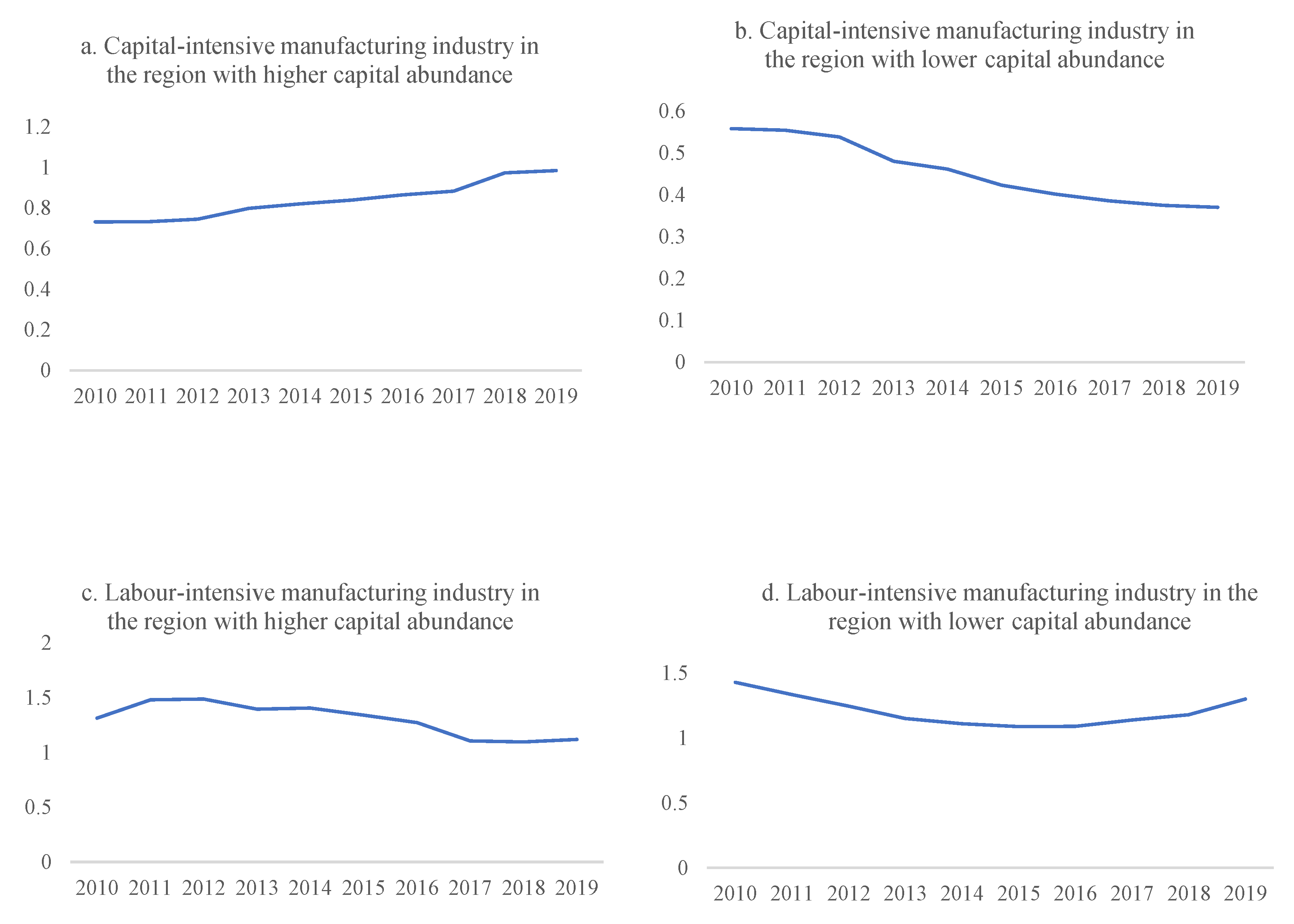
Figure 2.
Domestic trade costs and foreign trade costs in the eastern, central and western regions.
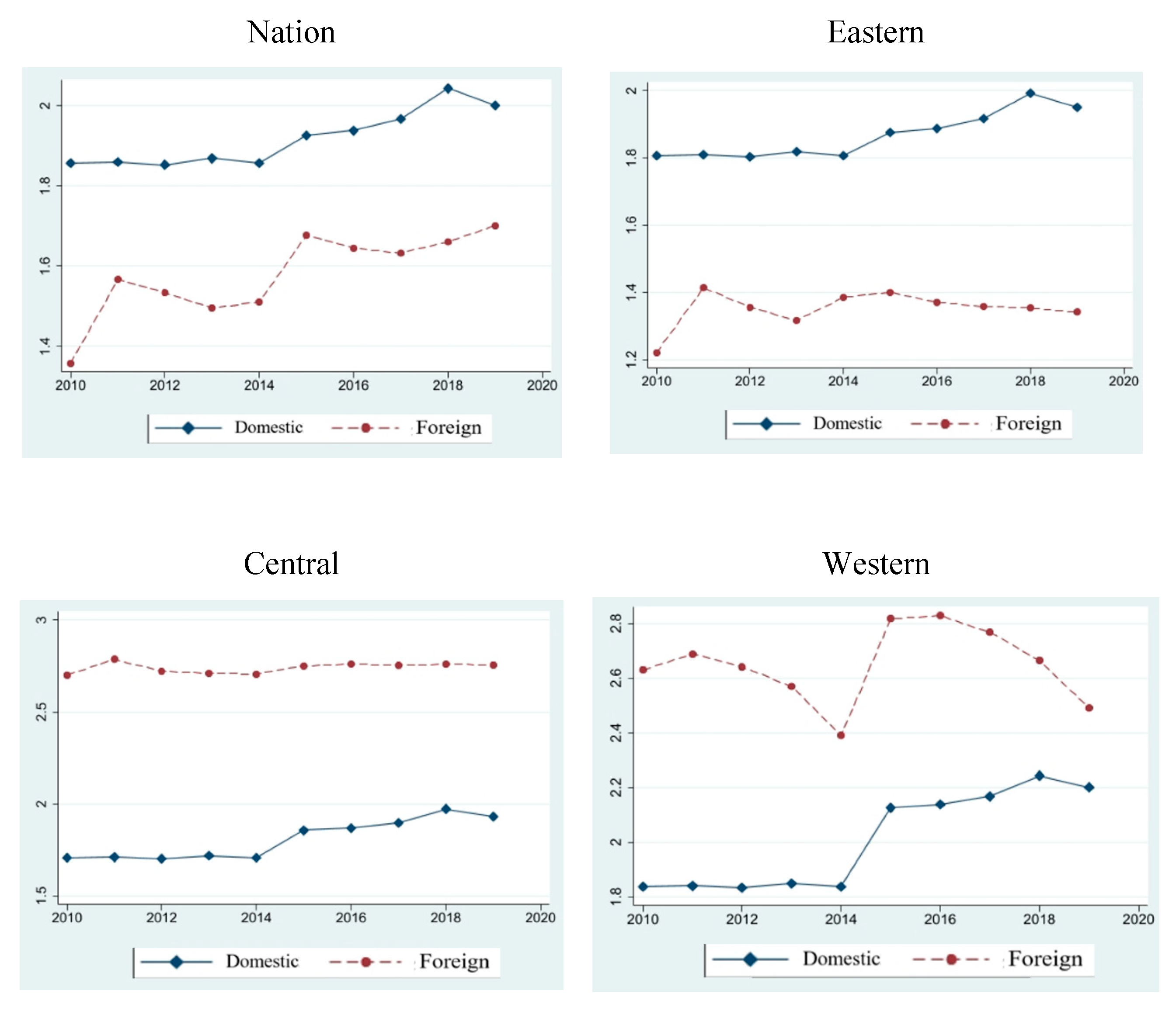

Table 1.
Dual Circulation Index.
| First grade | Second grade | Third grade | Indicator description | |
|---|---|---|---|---|
| Domestic Circulation | Intra-Province Circulation | Consumption | Consumption level | Consumption expenditure per capita / GDP per capita |
| Consumption structure | Immaterial consumption / Disposable income | |||
| Production | Production scale | Aggregate fixed investment /GDP | ||
| Production efficiency | Average productivity | |||
| Transportation | Logistics transportation | Transportation, warehousing, postal value added / GDP | ||
| Commodity turnover | Total retail sales / GDP | |||
| Distribution | Income distribution | Disposable income per capita / GDP per capita | ||
| Consumption investment balance | Overall payout / Aggregate fixed investment | |||
| Inter-Province Circulation | Integration | Domestic trade cost | Relative price index | |
| International Circulation | Trade | Trade balance | Net export / Total export-import volume | |
| Trade upgrading | High-tech industry introduction expenditure / Total export-import volume | |||
| Investment | FDI | FDI/GDP | ||
| OFDI | OFDI/GDP | |||
Table 2.
Provincial performance rankings.
| Rank | dual circulation index | Domestic circulation | International circulation | |||
|---|---|---|---|---|---|---|
| 1 | Beijing | 0.707 | Beijing | 0.894 | Hainan | 0.547 |
| 2 | Shanghai | 0.606 | Shanghai | 0.737 | Tianjin | 0.438 |
| 3 | Tianjin | 0.498 | Guangdong | 0.587 | Shanghai | 0.401 |
| 4 | Guangdong | 0.455 | Tianjin | 0.513 | Sichuan | 0.374 |
| 5 | Liaoning | 0.365 | Zhejiang | 0.478 | Beijing | 0.354 |
| 6 | Jiangsu | 0.364 | Liaoning | 0.418 | Chongqing | 0.351 |
| 7 | Zhejiang | 0.352 | Jiangsu | 0.415 | Shaanxi | 0.330 |
| 8 | Shandong | 0.336 | Shandong | 0.365 | Shanxi | 0.265 |
| 9 | Hainan | 0.323 | Fujian | 0.319 | Anhui | 0.260 |
| 10 | Sichuan | 0.305 | Heilongjiang | 0.310 | Jiangsu | 0.255 |
| 11 | Chongqing | 0.293 | Hebei | 0.294 | Hubei | 0.249 |
| 12 | Hubei | 0.281 | Inner Mongolia | 0.288 | Shandong | 0.244 |
| 13 | Anhui | 0.278 | Hubei | 0.284 | Guangdong | 0.234 |
| 14 | Fujian | 0.274 | Hunan | 0.281 | Guangxi | 0.231 |
| 15 | Shaanxi | 0.268 | Anhui | 0.274 | Guizhou | 0.226 |
| 16 | Guangxi | 0.265 | Guangxi | 0.263 | Zhejiang | 0.214 |
| 17 | Heilongjiang | 0.264 | Gansu | 0.262 | Liaoning | 0.210 |
| 18 | Hunan | 0.263 | Ningxia | 0.253 | Jiangxi | 0.199 |
| 19 | Hebei | 0.254 | Jilin | 0.253 | Hunan | 0.195 |
| 20 | Inner Mongolia | 0.254 | Jiangxi | 0.239 | Jilin | 0.192 |
| 21 | Gansu | 0.245 | Chongqing | 0.224 | Gansu | 0.184 |
| 22 | Henan | 0.244 | Yunnan | 0.217 | Fujian | 0.169 |
| 23 | Jilin | 0.242 | Sichuan | 0.212 | Ningxia | 0.166 |
| 24 | Shanxi | 0.242 | Shanxi | 0.211 | Henan | 0.160 |
| 25 | Jiangxi | 0.234 | Qinghai | 0.208 | Yunnan | 0.158 |
| 26 | Ningxia | 0.229 | Guizhou | 0.206 | Hebei | 0.141 |
| 27 | Guizhou | 0.221 | Xinjiang | 0.187 | Inner Mongolia | 0.139 |
| 28 | Yunnan | 0.205 | Henan | 0.186 | Qinghai | 0.101 |
| 29 | Qinghai | 0.184 | Shaanxi | 0.182 | Heilongjiang | 0.096 |
| 30 | Xinjiang | 0.162 | Hainan | 0.169 | Xinjiang | 0.074 |
Note: Due to the lack of some data, Xizang is not included in the calculation.
Table 3.
Benchmark regression results.
| DCI (Domestic weight 0.5) | DCI (Domestic weight 0.6) | DCI (Domestic weight 0.7) | DCI (Domestic weight 0.8) | DCI (Domestic weight 0.9) | Domestic circulation | International circulation | |
| Agg | 0.0116* (0.0067) |
0.0137** (0.0062) |
0.0201*** (0.0054) |
0.0214** (0.0102) |
0.0280** (0.0112) |
0.0177*** (0.0033) |
0.0025 (0.0208) |
| CV | Yes | Yes | Yes | Yes | Yes | Yes | Yes |
| Year Fixed | Yes | Yes | Yes | Yes | Yes | Yes | Yes |
| Individual Fixed | Yes | Yes | Yes | Yes | Yes | Yes | Yes |
| Obs. | 510 | 510 | 510 | 510 | 510 | 510 | 510 |
| R2 | 0.3446 | 0.4989 | 0.5965 | 0.5367 | 0.3728 | 0.3672 | 0.3765 |
Note: *, * *, * * * denote the significance level of 10 %, 5 % and 1 %, respectively, and the robust standard error is in parentheses.
Table 4.
IV-2SLS Estimation Results.
| IV-2SLS(IV: topographic relief) | IV-2SLS(IV: river density) | |||||
|---|---|---|---|---|---|---|
| First Stage | 0.7881*** (0.0022) |
0.6921*** (0.0004) |
||||
| F-value | 101.78 | 985.22 | ||||
| Second Stage | DCI | Domestic | International | DCI | Domestic | International |
| Agg | 0.0226*** (0.0036) |
0.0182*** (0.0009) |
-0.0015 (0.1217) |
0.0260** (0.0065) |
0.0191*** (0.0021) |
-0.0028 (0.2768) |
| CV | YES | YES | YES | YES | YES | YES |
| Year | YES | YES | YES | YES | YES | YES |
| Region | YES | YES | YES | YES | YES | YES |
| Obs. | 510 | 510 | 510 | 510 | 510 | 510 |
| R2 | 0.4036 | 0.4345 | 0.3575 | 0.3867 | 0.4708 | 0.4090 |
Note: *, * *, * * * denote the significance level of 10 %, 5 % and 1 %, respectively, and the robust standard error is in parentheses. The double circulation in the instrumental variable regression model is calculated by calculating the coupling coordination degree according to the domestic circulation weight of 0.7 and the international circulation weight of 0.3.
Table 5.
Regression results of subdivided samples.
| Domestic circulation | ||||
| (1) Aggku | (2) Aggkd | (3) Agglu | (4) Aggld | |
| 0.0180*** (0.0005) |
0.0093* (0.065) |
0.0184*** (0.0015) |
0.0097*** (0.0009) |
|
| CV | YES | YES | YES | YES |
| R2 | 0.5581 | 0.5172 | 0.4618 | 0.3713 |
| Intra-Province circulation | ||||
| (1) Aggku | (2) Aggkd | (3) Agglu | (4) Aggld | |
| 0.0178*** (0.0027) |
-0.0048 (0.0295) |
0.0180*** (0.0007) |
0.0134** (0.0051) |
|
| CV | YES | YES | YES | YES |
| R2 | 0.5396 | 0.4877 | 0.5145 | 0.3886 |
| Inter-Province circulation | ||||
| (1) Aggku | (2) Aggkd | (3) Agglu | (4) Aggld | |
| 0.0104*** (0.0021) |
0.0086** (0.0034) |
0.0272 (0.0415) |
0.0095* (0.0058) |
|
| CV | YES | YES | YES | YES |
| R2 | 0.5511 | 0.5221 | 0.4716 | 0.4339 |
Note: *, * *, * * * denote the significance level of 10 %, 5 % and 1 %, respectively, and the robust standard error is in parentheses.
Table 6.
The elasticity of returns to scale in manufacturing sub-sectors.
| Industry | Capital-output elasticity | Labour-output elasticity | Elasticity of returns to scale | Ratio of export delivery value to output value (%) |
|---|---|---|---|---|
| Agricultural and sideline food processing industry | 0.7566 | 0.2083 | 0.9649 | 4.90 |
| Food manufacturing industry | 0.6211 | 0.9771 | 1.5982 | 5.60 |
| Wine, beverage and refined tea manufacturing industry | 0.7227 | 0.5597 | 1.2824 | 1.60 |
| Tobacco products industry | 0.9404 | 0.1078 | 1.0482 | 0.45 |
| Textile industry | 1.1758 | 0.4210 | 1.5968 | 11.42 |
| Textile and clothing, clothing industry | 0.7329 | 0.3010 | 1.0339 | 23.36 |
| Leather, fur, feathers and their products and footwear | 0.8151 | 0.4783 | 1.2934 | 25.67 |
| Wood processing and wood, bamboo, rattan, brown, grass products industry | 0.8400 | 0.1888 | 1.0288 | 6.72 |
| Furniture manufacturing | 0.7544 | 0.5034 | 1.2578 | 23.05 |
| Papermaking and paper products industry | 0.9477 | 0.1376 | 1.0853 | 4.54 |
| Printing and Recording Media Reproduction | 1.0719 | 0.1885 | 1.2604 | 7.20 |
| Cultural and educational, industrial, sports and entertainment products manufacturing industry | 0.6857 | 1.0514 | 1.7371 | 32.43 |
| Petroleum processing, coking and nuclear fuel processing industries | 0.4022 | 0.1421 | 0.5443 | 1.76 |
| Chemical raw materials and chemical products manufacturing | 0.7082 | 0.6781 | 1.3863 | 5.59 |
| Pharmaceutical manufacturing industry | 0.5190 | 1.2212 | 1.7402 | 6.15 |
| Chemical fiber manufacturing industry | 0.6043 | 0.6269 | 1.2312 | 6.77 |
| Rubber and plastic products industry | 0.7007 | 0.4125 | 1.1132 | 13.82 |
| Non-metallic mineral products industry | 0.8154 | 0.5396 | 1.355 | 3.60 |
| Ferrous metal smelting and rolling processing industry | 0.3229 | 0.0893 | 0.4122 | 3.34 |
| Non-ferrous metal smelting and rolling processing industry | 0.7656 | 0.4437 | 1.2093 | 2.61 |
| Metal products industry | 0.7131 | 0.9239 | 1.637 | 10.99 |
| General equipment manufacturing industry | 0.4609 | 0.4406 | 0.9015 | 11.35 |
| Special equipment manufacturing industry | 0.5770 | 0.8350 | 1.412 | 9.45 |
| Transportation equipment manufacturing industry | 1.4134 | 0.0199 | 1.4333 | 8.61 |
| Electrical machinery and equipment manufacturing industry | 0.7430 | 0.5136 | 1.2566 | 16.11 |
| Computer, communications and other electronic equipment manufacturing | 0.6578 | 1.2625 | 1.9203 | 54.06 |
| Instrument and meter manufacturing industry | 0.7881 | 0.2708 | 1.0589 | 18.34 |
| Manufacturing average | 0.7502 | 0.5016 | 1.2518 | 11.83 |
| 1 | In fact, in the short-term equilibrium, due to the difference between the first nature and the second nature, there may be differences in the rate of return on capital and labor remuneration between region 1 and region 2, while in the long-term equilibrium, the rate of return on capital and labor remuneration will return to the same level. At this time, the employment of labor force in region 1 or region 2 can be regarded as undifferentiated, so the model setting does not restrict the flow of labor force between domestic regions in the long-term equilibrium. |
| 2 | In the process of solving, in order to make the form of the wage equation as simple as possible, the marginal cost of production , and the fixed cost are set. |
| 3 | Due to symmetry, near the equilibrium point, the total differential of the related expressions of region 1 and region 2 can be combined and abbreviated, and the corner markers 1 and 2 are omitted here. |
| 4 | Similarly, the total differential abbreviation omits the corner mark due to symmetry. In order to simplify the analysis, it is assumed that the transportation costs of Region 1 and 2 are equal, that is, τ12 = τ21, and expressed by τ. |
| 5 | The capital-intensive industries in this paper include chemical raw materials and chemical products manufacturing industry, other non-metallic minerals, mechanical and electrical industry, transportation equipment industry, water transportation industry, support and auxiliary transportation activity industry, and the remaining manufacturing sub-sectors are labor-intensive. |
Disclaimer/Publisher’s Note: The statements, opinions and data contained in all publications are solely those of the individual author(s) and contributor(s) and not of MDPI and/or the editor(s). MDPI and/or the editor(s) disclaim responsibility for any injury to people or property resulting from any ideas, methods, instructions or products referred to in the content. |
© 2025 by the authors. Licensee MDPI, Basel, Switzerland. This article is an open access article distributed under the terms and conditions of the Creative Commons Attribution (CC BY) license (http://creativecommons.org/licenses/by/4.0/).
Copyright: This open access article is published under a Creative Commons CC BY 4.0 license, which permit the free download, distribution, and reuse, provided that the author and preprint are cited in any reuse.


