Submitted:
01 July 2025
Posted:
07 July 2025
You are already at the latest version
Abstract
This study forecasted tax revenues by estimating Korea's national tax revenue functions using time series techniques to enhance methodological accuracy. Analysis results demonstrated that cointegration methods had superior predictive power, providing statistically significant estimates for tax revenue projections. Tax revenue projections estimated using the cointegration method of DOLS (Dynamic Ordinary Least Squares) and FMLS (Fully Modified Least Squares) demonstrated superior predictive accuracy, particularly outperforming government forecasts in tax categories with significant revenue shortfalls. However, changes in assumptions of explanatory variables were found to substantially alter tax revenue projections. This underscores the importance of accurate forecasting through appropriate model selection tailored to economic conditions and continuous updates of explanatory data.
Keywords:
cointegration
; corporate tax
; dynamic forecast
; income tax
; tax revenue projection
1. Introduction
Forecasting tax revenue is inherently complex and challenging due to ongoing economic uncertainties. Large or recurring tax revenue errors can lead to adverse effects on fiscal management and weaken public trust in government policies.
To improve forecasting accuracy, economic conditions and econometric methodologies are crucial [1]. Along with macroeconomic econometric models sensitive to business cycles, time-series forecasting approaches such as univariate Autoregressive integrated moving average (ARIMA) models [2], multivariate Vector autoregression (VAR) models [3], and Bayesian VAR models [4], are widely used in OECD countries due to their low forecasting errors [5]. On the other hand, machine learning techniques have been only somewhat effective in specific cases, such as land transfer taxes in Australia [6] and the U.S. [7], where business cycles are sensitive.
Accordingly, the purpose of this study was to investigate the current method of estimating national tax revenue based on a time-series approach. The tax revenue forecasting model was then modified by addressing its issues based on tax structure and changing economic conditions, aiming to minimize forecasting errors and contribute to improved efficiency of government fiscal operations. This study enhances the performance of tax revenue forecasting by analyzing its relationships with determining factors that exhibit time-series patterns similar to future values of tax revenue.
Germany considers the majority of tax revenue forecasting errors to be due to incorrect predictions of macroeconomic variables. It has reduced forecasting errors by improving predicted values of explanatory variables and estimation methodologies [8]. In particular, this study was conducted from the perspective that forecasting using the dynamic equilibrium relationship between tax revenues by category and their determining factors could be useful in an environment having a high uncertainty in tax revenue forecasts.
Therefore, in terms of improving research methodology, the study will add long-term relationships between time-series data to the macroeconomic tax revenue forecasting model, check key tax category models, and propose a new tax revenue forecasting approach. The model will be formulated by combining short-term forecasts of explanatory variables in a dynamic equilibrium state, with forecasted values of budget explanatory variables determined using both macroeconomic projections reflecting government policy effects and time-series forecasting. By introducing stable equilibrium time-series methods and adjusting in-sample forecasts, this study aimed to reduce forecasting errors and improve model performance.
As a means to effectively forecast the size and composition of future national tax revenues, the study will update parameter elasticity weights and biases for tax revenues by correcting forecasting errors using data reflecting the latest economic conditions through a probability loss function. During periods of economic shocks where forecasts are challenging, dummy variables or interval forecasts can be used, while factors such as non-compliance with tax regulations, decline of high-income corporate tax revenues, tax-avoidance revenues, and increase of revenue from collection convenience can be examined using information technology [9].
The goal of this study’s tax revenue forecasting model and empirical analysis for estimating its effectiveness is not only to review sources of uncertainty in tax revenue forecasts and propose solutions, but also to offer valuable insights for policy adjustments and significant academic implications.
2. Empirical Improvement of Tax Revenue Forecasting Loss
National taxes are imposed and collected according to standardized criteria. The method of forecasting these tax revenues is typically based on models using macroeconomic indicators as explanatory variables, which are derived from average values. Therefore, changes in economic conditions and policies can lead to forecasting errors. Since national taxes are estimated as the total revenue by summing individual tax revenue forecasts for a given year, although theoretical precision might be somewhat sacrificed, efforts are made to improve forecasting effectiveness. This section aims to review the methodology of tax revenue estimation through an empirical analysis of Korea’s GDP-based forecasting model and predictions from 2010 to 2023 following the financial crisis in order to identify areas for improvement. This study will analyze error losses from static forecasts using regression models and dynamic forecasts based on time-series historical patterns and explore ways to improve them.
To effectively apply the tax revenue model set for each tax category to the economic situation, it is necessary not only to continuously improve modeling and estimation methodologies, but also to establish forecasting assumptions through post-analysis of errors. Minimizing forecasting error loss in regression analysis can improve the model’s precision and reduce estimation bias, thereby increasing the robustness of forecasts. However, tax revenue forecasting is difficult because it also depends on future economic conditions, speculative behavior, and policy changes, which are hard to model. Tax revenue forecasting errors through the tax rate system include forecasting errors of macroeconomic variables due to business cycle fluctuations, policy forecasting errors resulting from unexpected tax law amendments, and remaining unexplained model prediction errors.
Forecasting error (et,h) is defined as the difference between the future observed value of tax revenue (yt+h) and its forecasted value (ft,h). Time-series forecasting models focus on using information up to the current time (t) to predict values after time t (h) as shown below:
et,h = yt+h − ft,h = yt+h − y^t+h
where ft,h represents the point forecast estimate (y^t+h) obtained through the regression model. To achieve optimal forecasting, the method that can reduce forecasting errors is by setting the loss function as the objective function and using the optimal forecast (f*t,h) that can minimize the expected value of the loss function as shown below:
where L(et,h) represents the loss function of the forecasting error, Et is the expectation operator, and argmin is the operation symbol for finding the argument that gives the minimum value of a function.
f*t,h = argmin Et(L(et,h))
ft,h
Errors (residuals) are calculated for in-sample forecasts, while forecasting errors can be calculated for out-of-sample forecasts. By making adjustments to reduce errors through in-sample forecasting, the loss of forecasting errors can be minimized. Since forecasting errors will lead to analysis errors, reducing the forecasting error in judgment can help adjust the optimal forecast [10]. To find the optimally adjusted forecast that can minimize the standard deviation of forecasting errors, estimating the variance of forecast errors is challenging. For convenience, one can use the forecast error loss function and set it to minimize the expected value so that the optimal forecast can be utilized.
In other words, linear regression analysis makes it easy to interpret causal relationships and calculate predictions once coefficients of explanatory variables are known. However, its accuracy may be low. Multiple regression models can predict average response of tax revenue using the intercept (bias) and explanatory variables predicted for parameters. Since time-series analysis generally has explanatory power and accuracy, it is necessary to compare predictions of univariate time-series tax revenue models.
Therefore, the optimal forecasting method involves setting up precise econometric models, obtaining static predictions for economic variables, and reducing forecasting errors in regression analysis to decrease biases. As a result, individual tax models will be initially checked using sample data. Through adjustments between static and dynamic forecasts, forecasting errors in judgments of explanatory variable predictions can be minimized, thus improving the model that can optimally adjust tax revenue estimates.
First, for individual tax functions, factors affecting tax revenue will be empirically re-examined. These factors include business cycle fluctuations, rapid changes in the economic situation, policy changes, technical disruptions such as e-commerce and other innovations, changes in consumer behavior, demographic trends such as low birth rates and an aging population, volatility in stock and energy markets, and external shocks such as geopolitical crises and natural disasters. Since tax revenue is influenced by economic conditions, adjustments are made by modifying or adding macroeconomic variables, especially for tax categories with large errors, to improve the model’s fit to reality. Accordingly, the selection of explanatory variables for income tax, corporate tax, and value-added tax, where errors are most significant, has been preliminarily checked through in-sample correlations.
Budget and final tax revenues show similar correlations among key tax categories. Additionally, correlations between key macroeconomic indicators (e.g., GDP, personal income, domestic demand) and tax revenues (both budget and final) are nearly identical. While budget tax revenues are slightly higher than final tax revenues, these two revenues are almost the same. Thus, correlations between budget tax revenues and macroeconomic indicators will be examined in detail.
By tax category, GDP, nominal wages, the number of wage earners, private consumption, the consumer price index, and exchange rates show very high correlations with income tax. Their correlations with specific taxes such as labor income tax, comprehensive income tax, and capital gains tax are around 0.9. Their correlations with interest and dividend taxes are about 0.6, whereas their correlations with other income taxes are very low. Similarly, GDP, nominal wages, the number of wage earners, private consumption, inflation, and exchange rates have high correlations (about 0.9) with corporate tax (both reported and withheld) and value-added tax. However, interest rates have very low correlations with income tax, corporate tax, and value-added tax.
Therefore, labor income tax, comprehensive income tax, capital gains tax, corporate tax, and value-added tax can tentatively use key macroeconomic variables (e.g., GDP, nominal wages, the number of wage earners, private consumption, consumer prices, exchange rates) as explanatory variables. However, interest tax, dividend tax, and other income taxes should be modeled and analyzed with other factors.
Second, we will check whether forecasts of macroeconomic indicator explanatory variables (i.e., static predictions) are accurate. A multiple regression model uses two or more explanatory variables to predict the average response of tax revenue, the dependent variable. Multivariate regression analysis predicts tax revenue by inputting predicted values of explanatory variables into the intercept (bias) and parameter estimates. By adding dynamic forecasts using univariate time-series for income tax and corporate tax, which are closely related to profits and wages but difficult to predict, we can improve prediction values and reduce tax revenue forecasting errors.
The forecasting accuracy of tax revenue based on errors in national tax and tax category forecasts (= actual outcome − budget forecast) and error rates (= forecasting error ÷ actual value or forecast value) is evaluated as follows. Table 1 shows results of analyzing central tendency, persistence, and forecasting accuracy of tax revenue forecasting errors.
In the case of national taxes, the average error rate indicating central tendency of tax revenue forecasts is 2.016 trillion KRW and the mean absolute percentage error (MAPE) indicating forecasting accuracy is 4.52%. Autocorrelation of errors, which tests the persistence of errors, is 0.14 for 1 lag, -0.29 for 2 lags, and 0.04 for 3 lags, indicating that errors are not persistent. For reference, the autocorrelation of national taxes is 0.79 for 1 lag, 0.50 for 2 lags, and 0.33 for 3 lags, showing persistence. Previous year’s national tax revenue had a significant effect on the current year’s tax revenue. The persistence of tax revenue gradually declined.
In contrast, for income tax, the average error rate is 2.209 trillion KRW, which is higher than that for total tax revenue, and the MAPE is 5.71%, showing a lower accuracy than that for total tax revenue. Among income taxes, the capital gains tax has an average error rate of 1.298 trillion KRW and an MAPE of 20.87%, showing a significantly high forecasting error with a very low accuracy. Meanwhile, for corporate tax, the average error rate is -1.348 trillion KRW and the MAPE is 6.84%, shower a lower accuracy than that for total tax revenue. Among corporate taxes, the reported amount has an average error rate of -1.683 trillion KRW and an MAPE of 9.09%, showing a very large forecasting error and a low accuracy. In contrast, the value-added tax has an average error rate of 0.223 trillion KRW and an MAPE of 3.56%, showing a higher accuracy than that for total tax revenue. The autocorrelation of errors by tax category is not strong or persistent.
Time series dynamic forecasting helps understand the fundamental structure of tax revenue data and predict future values based on past patterns, offering high explanatory power and accuracy. Therefore, as the uncertainty of tax revenue increases, particularly when capital gains tax and corporate income tax’ filing amounts have significant errors and low predictive accuracy, it is necessary to assess their forecasting capabilities.
Figure 1 compares static forecasts for capital gains tax and corporate income tax filing amounts, the most uncertain revenue categories, with dynamic forecasts from within-sample time series data. In the time series data processing process, white noise (residuals with a mean of zero, a normal distribution, and no autocorrelation) allows for dynamic analysis and forecasting. In the tax revenue model, the stable time series model ARMA(1,1) was preliminarily selected. The ARMA model had a model fit (R2) of 0.89, which was higher than that of ARIMA. Estimated coefficients were significant. In contrast, Box-Jenkins’ ARIMA(1,1,1) and AR(1) models showed that the coefficient of AR(1) was not significant. Additionally, based on an AIC value of 224.3, a lag length of 1 was selected for convenience.
Recently, for the year 2023, the forecast error for tax revenue was quite large and dynamic forecasting using ARMA(1,1) was more accurate than static forecasting. By tax category, the forecast error for capital gains tax was very large and the error for corporate income tax filings was somewhat larger. Moreover, dynamic forecasting for capital gains tax was far more accurate than static forecasting. Dynamic forecasting for corporate income tax filings was also more accurate than static forecasting.
The fact that static forecasts using a multivariate regression model have lower accuracy than dynamic forecasts suggests that dynamic adjustment is needed to reduce future discrepancies based on past prediction errors. As prediction errors in models such as those for income tax and corporate tax, which have lower forecasting power, lead to analytical errors, it becomes important to use a cointegration model that incorporates time-varying information to reduce prediction error losses and focus on dynamic forecasting.
3. Tax Revenue Model Specification in Long-Run Equilibrium
This section aims to suggest directions for improving forecast performance based on issues in tax revenue forecasting methods using macroeconomic regression analysis, which is traditionally known for its accuracy in short-term predictions. Empirical results indicate that predictions using cointegration have higher forecasting power than simple predictions based on dynamic past variables. This section discusses the necessity and effectiveness of forecasting through dynamic regression models that incorporate cointegration relationships.
In a simplified view of tax revenue forecasting methods, the tax revenue for the current year can be estimated by applying the expected economic growth rate for the following year, which helps determine the tax revenue forecast. The formula for simple tax revenue forecasting is shown as follows:
Tt+1 = Tt (1 + gt+1)
Where Tt+1 represents the forecasted tax revenue for the following year, Tt represents the current year’s tax revenue, and gt+1 represents the expected economic growth rate for the following year. National taxes can be calculated simply by summing estimated forecasted values for each tax category.
However, this approach has several issues. One issue with this approach is that it assumes a tax elasticity of 1 with respect to the economic growth rate. To improve this, the tax elasticity for each tax category, which can vary depending on the economic situation, will be empirically estimated to provide a more objective forecast. Another issue is that if the explanatory variable for each individual tax model is simplified to the economic growth rate, the explanatory power will be limited. Therefore, explanatory variables reflecting specific characteristics of determinants for each tax category will be selected and added for statistical processing. Additionally, it is necessary to explicitly reflect feedback effects between individual tax revenues.
In particular, the purpose of estimating the tax revenue model is to forecast tax revenues. Even if the theoretical model and statistical analysis are conducted precisely, there are constraints on forecasted values of explanatory variables needed for the prediction. To enhance effectiveness of the forecast, tax function will be determined using highly explanatory and significant determinants.
Furthermore, if predictions using dynamic regression models prove to be more effective than those using static regression models, the former will be used for forecasting. For example, since income tax and corporate tax are sensitive to economic fluctuations, while value-added tax and sales tax are more dependent on the previous year’s revenue, it is necessary to attempt forecasting using dynamic regression models.
The forecast formula using the static regression model is expressed as follows:
yt = β0 + β1xt + ut
Et(yt+1) = β0 + β1xt+1
Where yt is the tax revenue for the current period (t), xt is the explanatory variable, β0 and β1 are coefficients, Et is the expectation operator, and ut is the error term.
In the simple model of Equation (4), if the future explanatory variable xt+1 is known, xt+1 can be predicted. However, in reality, xt+1 is often not available, which leads to the complication of having to predict the explanatory variable as well.
On the other hand, forecasting through a dynamic regression model helps avoid this inconvenience. The forecast formula using a dynamic regression model can be expressed as follows:
yt = β0 + β1yt-1 + β2xt-1 + ut
Et(yt+1) = β0 + β1yt + β2xt
In this case, the error term’s mean should be zero. It should not be correlated with explanatory variables. In this analysis, both static and dynamic models will be estimated and compared.
Multivariate forecasting is often not more powerful than univariate forecasting. This is because when there are more estimated forecasted values for additional parameters, errors due to sampling variability will be introduced, model selection will become more difficult, and the influence of outliers will increase. However, if a cointegration relationship holds, the forecast from a multivariate cointegration model with fixed coefficients can have more forecasting power due to characteristics of the cointegration relationship.
Cointegration occurs when two or more time series share a common long-term trend or equilibrium relationship. It refers to the phenomenon where time series variables maintain a long-term equilibrium relationship. If economic variables are cointegrated, they will maintain an equilibrium relationship in the long run. When one economic variable regresses onto another, the error term remains within a stable range, which is helpful for forecasting.
Cointegration refers to a situation where linear combination of time series variables maintains a stable equilibrium relationship, even if there are short-term deviations, because these variable share a common trend and have economic relevance. This allows for the analysis of long-term relationships using traditional econometric theories. When analyzing unstable time series variables, differencing the series to remove unit roots can convert them into stable time series. However, this process can lead to a loss of long-term informational characteristics between variables. Therefore, it is important to maintain stability of regression analysis while considering long-term characteristics of economic statistics through cointegration.
When performing regression analysis of non-stationary time series variables that do not have a long-term equilibrium relationship, spurious regression issues can arise, making it necessary to check for cointegration. If cointegration exists, it means that residuals after estimation will form a stable time series. In this context, a cointegration vector representing a linear combination of time series variables can indicate their equilibrium relationship.
In Equation (4), an appropriate estimation depends on characteristics of explanatory variables and the error term included in the model. If the explanatory variable is an unstable I(1) stochastic process with a unit root and the error term is also I(1), then Equation (4) would result in a spurious regression model. In this case, it is not possible to obtain consistent estimators using the ordinary least squares (OLS) method. Therefore, as shown in the equation below, all variables must first be transformed into stable stochastic processes by taking the first difference (∆) so that coefficients can be estimated:
∆yt = β0 + β1∆xt + ∆ut
If the explanatory variable is an unstable I(1) stochastic process with a unit root and the error term is I(0), then Equation (4) becomes a cointegrated regression model. Even if there is endogeneity between the explanatory variable and the error term, consistent estimators for level variables can be obtained using the OLS method without needing instrumental variables.
When time series variables exhibit a cointegration relationship, an error correction model (ECM) can be used to analyze both long-term and short-term effects. The error correction term represents the adjustment effect of imbalances. If the actual value of the dependent variable in the previous period is greater than its predicted value (resulting in a positive prediction error), the actual value will be reduced in the following period to maintain the long-term relationship between dependent and explanatory variables. In other words, the error correction term is added to maintain the cointegration relationship. The error correction term is properly defined when time series variables are differenced at the same order and a cointegration relationship is established. Additionally, events such as economic crises can lead to an above-average volatility. Using dummy variables might not effectively address non-normality of the data. For this reason, cointegration relationships are estimated using data from periods following events such as the foreign exchange crisis and the financial crisis.
Furthermore, if there is no endogeneity between explanatory variables and the error term, consistent estimators can be obtained using the OLS method. However, if endogeneity exists, consistent estimators can be obtained using instrumental variables (IV) estimation or other estimation methods. When a cointegration relationship is established, consistent estimators can be obtained without using instrumental variables, even if there is endogeneity. In the case of tax revenue, if explanatory variables and the error term are stable, non-unit-root stochastic variables, the condition for no endogeneity between explanatory variables and the error term is then satisfied. This allows consistent estimators to be obtained using the OLS method.
In other words, the tax revenue function can be identified using the following least squares methods. Dynamic Ordinary Least Square (DOLS) approach can improve both the OLS procedure with super-consistent and serially correlated estimates and the maximum likelihood procedure by removing dynamic sources of bias [11]. DOLS is a single equation method that can correct for regressor endogeneity by adding leads and lags of first differences of regressors. It can also correct for serially correlated errors with a GLS procedure. Fully Modified OLS (FMLS) method can also correct for endogeneity in regressors and serial correlation resulting from a cointegration [12].
In summary, the classical method of OLS for finding actual weights is an effective way to determine the regression equation (regression coefficients) by minimizing the sum of squared residuals (errors). It assumes homoscedasticity, independence, a mean of zero for errors (no fixed errors), and a normal distribution. Therefore, to accurately estimate tax revenues from a long-term equilibrium perspective, DOLS and FMLS estimation methods are used together to complement the statistical testing of OLS estimates, incorporating endogeneity between explanatory variables and errors as well as serial correlation of error terms.
Data used in the empirical analysis of the tax revenue model consisted of Korea’s tax revenue and economic variables that could determine tax revenue. The analysis period spanned from 1999, following the Asian financial crisis, to 2024, using annual data officially released by sources such as the KOSIS National Statistical Portal, the Bank of Korea Economic Statistics System, and the Korea Customs Service.
4. Testing Results
This section empirically estimates the national tax revenue model and forecasts projected estimates empirically. In the empirical analysis, effective methodologies will be used to improve the performance of the regression analysis model and enhance the accuracy of numerical predictions despite insufficient data.
First, during the data processing stage, outliers were removed, missing values were handled by replacing them with the mean, and scale differences of input variables were reduced to improve the model’s performance, stability, and convergence speed. Second, in the variable selection stage, correlation coefficients and Variance Inflation Factors (VIF) were checked to remove unnecessary variables with low correlations or high multicollinearity, thereby improving the model’s performance. New variables were created through combinations of existing variables to enhance predictive power. Additionally, categorical variables were converted into dummy variables and interaction terms were added by multiplying variables to further increase prediction accuracy. Third, during the model estimation stage, stable equilibrium relationships were utilized by verifying unit roots and cointegration according to time-series econometric methods to identify optimal parameters. Furthermore, results of estimating static and dynamic cointegrated regression models were compared to select the optimal estimate. Fourth, in the prediction stage, dynamic predictions were used to supplement static forecasts made by experts. Data were divided into in-sample and out-of-sample segments. Both in-sample and out-of-sample predictions were conducted simultaneously to improve the prediction performance.
A time-series stability test was conducted to assess the stability of variables needed for the empirical analysis of the tax revenue model. The stability of the time-series variables used in the analysis was checked through unit root tests.
Table 2 shows results of the (Augmented) Dickey-Fuller unit root test. As a result of the Wald test for the unit root model, for most variables, we could not reject the null hypothesis that there is a unit root at the 5% significance level. It was found that unstable level variables became stationary after first differencing. Therefore, it is necessary to test whether a cointegrating relationship exists among level variables.
To confirm the long-term equilibrium relationship between dependent and explanatory variables in individual tax models, a cointegration test was conducted for the regression model below. The equilibrium relationship between time series variables to be used in the regression model was verified by cointegration tests.
Table 3 presents results of cointegration tests proposed by [13,14]. Results of testing the linear trend model with structural breaks, as proposed by [14], using the appropriate lag based on AIC, showed that for all individual tax models, the null hypothesis of the presence of a unit root in the residuals (indicating no cointegration) was rejected at the 5% significance level. Therefore, cointegration regression analysis was performed using level variables of tax models.
As it was confirmed earlier that individual variables in tax models exhibited unit roots without showing a cointegration relationship, a Granger causality test was first conducted to estimate the cointegration regression model. Based on a four-lag specification of explanatory variables, results of the test rejected the null hypothesis of no causality for most individual tax models, assuming the existence of causal relationships.
Now that a stable cointegration relationship was established, static and dynamic OLS estimators for regression models were used to estimate tax functions and discuss results. Estimated regression equations, cointegration regression model estimation results, and projections on tax revenue were discussed by separating them into individual tax categories.
From now on, we will specify the cointegration tax revenue regression model, assess its robustness, estimate it, and make predictions. We performed optimal estimation on cointegration regression models for each tax category and then made forecasts for tax revenue.
Analysis procedures were as follows. First, when determining the tax revenue estimation model, if there are many independent variables, overfitting will reduce errors but increase the variance of parameters, leading to lower prediction reliability. Conversely, if there are fewer independent variables, underfitting will increase errors (bias), although the standard deviation of parameters is lower. Therefore, endogenous variables were adjusted to reduce errors and increase reliability based on the economic theory.
Second, since time series data changed over time, the method to reduce prediction errors based on past information (learning) used the prediction that minimized expected value of the loss function. For optimal prediction, the tax revenue estimation error (= actual settlement value − budget forecast value) was used as a control variable for estimation.
Third, the method of adjusting the tax revenue loss function aimed to improve the model’s prediction performance by processing and utilizing the data according to the analysis objective and characteristics of the time series data, considering trend, seasonality, and outlier removal. Additionally, regularization techniques were used to prevent excessive weights in the linear regression model’s cost function. Regularization could control the model’s complexity, reduce data dimensions, and mitigate the risk of overfitting.
Fourth, the ideal tax revenue prediction strategy differed by country but depended on the availability of data information. It is important to predict each individual tax, as each tax category contributes differently to the forecast based on its taxable base. Since Korea’s estimation errors arose from asymmetric errors across tax categories, utilizing information from tax categories with significant weight and errors could improve prediction accuracy. However, predicting tax revenue is challenging due to complex interactions between economic fluctuations and government policies. Therefore, optimal forecasting values estimated were compared with those from a random simulation considering shocks as a forecasting method for single time series.
4.1. Income Tax
The estimation model for income tax revenue was divided into labor income tax, comprehensive income tax, capital gains tax, and interest and dividend income tax as shown below. Through principal component analysis and factor (covariance-correlation matrix) analysis, variables having low correlations with tax revenue were eliminated to reduce dimensionality of data. Multicollinearity checks were then performed to exclude explanatory variables having high correlations from the analysis. The estimated equation for level variables with realized prediction error (= actual value − realized forecast value) as a control variable is presented along with estimation results.
4.1.1. Labor Income Tax
Estimation results for level variable equation of labor income tax after adjustment considering key factors such as multicollinearity were obtained from y = f(X1, X2), where y was the labor income tax, X1 was the wage, X2 was the forecasting error of labor income tax, and f(.) was the functional form. Based on estimated values of the labor income tax cointegration model, in-sample labor income tax revenue predictions reflecting basic forecast values of labor income tax explanatory variables are shown in Table 4.
The comparison of model forecasting accuracy using RMSE for in-sample labor income tax revenue forecasts showed that, compared to the government’s forecast of 1,573,702 million KRW for the labor income tax, OLS had a forecast of 13,056,065 million KRW, DOLS had a forecast of 12,079,926 million KRW, and FMLS had a forecast of 12,634,118 million KRW. These results revealed that the government’s prediction method had the highest forecasting accuracy, followed by the DOLS method.
For the next year’s tax revenue, excluding the OLS method due to endogeneity issues, results comparing the DOLS method (which had the second highest forecasting accuracy after the government’s forecast) with other estimation techniques are shown in Table 5.
The forecast for labor income tax revenue in 2025 was estimated at 74,227,332 million KRW using the DOLS method and 68,123,375 million KRW using the dynamic model DOLS method. The actual time series forecast (random simulation) of 74,432,574 million KRW served as a reference estimate. However, the forecast from the labor income tax cointegration regression model could be sensitive to assumptions regarding predicted values of the explanatory variable such as salary, the chosen estimation model, the chosen estimation method, and shocks related to labor and labor income.
4.1.2. Comprehensive Income Tax
Estimation results for the level variable equation of comprehensive income tax after adjustment considering key factors such as multicollinearity were obtained from y = f(X1, X2), where y was the comprehensive income tax, X1 was the business income and real estate rental income, X2 was the forecasting error of comprehensive income tax, and f(.) was the functional form. Based on estimated values of the labor income tax cointegration model, in-sample comprehensive income tax revenue predictions reflecting the basic forecast values of the comprehensive income tax explanatory variables are shown in Table 6.
The comparison of model forecasting accuracy using RMSE for in-sample comprehensive income tax revenue forecasts showed that, compared to the government’s forecast of 2,870,935 million KRW, OLS had a forecast of 4,378,596 million KRW, DOLS had a forecast of 16,559,414 million KRW and FMLS had a forecast of 10,932,554 million KRW. These results showed that the government’s prediction method had the highest forecasting accuracy, followed by FMLS and then DOLS.
To estimate the tax revenue for the next year, the FMLS method’s forecast was then compared with forecasts of other estimation techniques. Results are shown in Table 7.
The forecast for comprehensive income tax revenue in 2025 was estimated at 17,173,790 million KRW using the FMLS method. The actual time series forecast (random simulation) of 25,177,055 million KRW served as a reference estimate. However, the forecast from the comprehensive income tax cointegration regression model could be sensitive to assumptions regarding predicted values of explanatory variables such as business income and real estate rental income, the chosen estimation model, the chosen estimation method, and shocks related to business income and real estate rental income.
4.1.3. Capital Gains Tax
Estimation results for the level variable equation of comprehensive income tax after adjustment considering key factors such as multicollinearity were obtained from y = f(X1, X2, X3), where y was the capital gains tax, X1 was the transfer price, X2 was the capital gain, X3 was the forecasting error of capital gains tax, and f(.) was the functional form. Based on estimated values of the capital gains tax cointegration model, in-sample capital gains tax revenue predictions reflecting basic forecast values of capital gains tax explanatory variables are shown in Table 8.
Comparison of model forecasting accuracy using RMSE for in-sample capital gains tax revenue forecasts showed that, compared to the government’s forecast of 8,715,320 million KRW, OLS had a forecast of 6,428,878 million KRW and FMLS had a forecast of 6,067,648 million KRW. These results revealed that the FMLS method had the highest forecasting accuracy, followed by the OLS method, while the government’s forecast had the lowest accuracy. This indicates that the forecasting error for capital gains tax has increased recently, leading to a larger shortfall in capital gains tax revenue.
To estimate tax revenue for the next year, the FMLS method’s forecast was then compared to forecasts with other estimation forecasts. Results are shown in Table 9.
The forecast for capital gains tax revenue in 2025 was 19,081,552 million KRW using the FMLS method, as it had the highest forecasting accuracy. The actual time series forecast (random simulation) of 20,551,933 million KRW served as a reference estimate. However, the forecast from the capital gains tax cointegration regression model could be sensitive to assumptions regarding predicted values of explanatory variables such as asset transfer price and capital gain, the chosen estimation model, the chosen estimation method, and shocks related to asset transfer price and capital gain.
4.1.4. Interest and Dividend Income Tax
Estimation results for the level variable equation of interest and dividend income tax after adjustment considering key factors such as multicollinearity were obtained from y = f(X1, X2, X3), where y was the interest and dividend income tax, X1 was the interest and dividend income, X2 was the balance of deposits and bonds, X3 was the forecasting error of interest and dividend income tax, and f(.) was the functional form. Based on estimated values of the interest and dividend income tax cointegration model, in-sample interest and dividend income tax revenue predictions reflecting basic forecast values of the interest and dividend income tax explanatory variables are shown in Table 10.
The comparison of model forecasting accuracy using RMSE for in-sample interest and dividend income tax revenue forecasts showed that, compared to the government’s forecast of 1,141,991 million KRW, OLS had a forecast of 2,172,656 million KRW and FMLS had a forecast of 1,302,785 million KRW. These results revealed that the government’s prediction method had the highest forecasting accuracy, followed by the FMLS method, whereas the OLS method had the lowest accuracy.
To estimate the tax revenue for the next year, the FMLS method’s forecast was compared with other estimation forecasts. Results are shown in Table 11.
The forecast for interest and dividend income tax revenue in 2025 was estimated at 8,016,698 million KRW using the FMLS method. The actual time series forecast (random simulation) of 11,040,117 million KRW served as a reference estimate. However, the forecast from the interest and dividend income tax cointegration regression model could be sensitive to assumptions regarding predicted values of explanatory variables such as interest and dividend income, the chosen estimation model, the chosen estimation method, shocks related to interest and dividend income, and balances of deposits and bonds.
4.2. Corporate Tax
Estimation results for the level variable equation of corporate tax after adjustment considering key factors such as multicollinearity were obtained from y = f(X1, X2, X3), where y was the corporate tax, X1 was the corporate net income, X2 was the capital investment, X3 was the corporate tax forecasting error, and f(.) was the functional form. Based on estimated values of the corporate tax cointegration model, in-sample corporate tax revenue predictions reflecting basic forecast values of corporate tax explanatory variables are shown in Table 12.
The forecasting accuracy of corporate tax revenue can be assessed using prediction error loss. The comparison of model prediction performance using the RMSE for in-sample corporate tax revenue predictions showed that the government’s forecast was 17,382,371 million KRW, whereas OLS’ forecast was 23,140,958 million KRW, DOLS’s forecast was 12,308,331 million KRW, and FMLS’s forecast was 20,905,217 million KRW. These results revealed that the DOLS method had higher forecasting accuracy than the government’s prediction method, suggesting that the recent increase in corporate tax forecasting errors might have led to a larger corporate tax deficit.
As the DOLS prediction showed a higher forecasting accuracy, the predicted corporate tax revenue for the following year compared with other time series forecasts is shown in Table 13.
The forecast for corporate tax revenue in 2025 was estimated at 81,549,804 million KRW using the DOLS method. The actual time series forecast for reference was estimated at 81,974,971 million KRW. However, the forecast from the corporate tax cointegration regression model could be sensitive to assumptions regarding predicted values of explanatory variables such as net income and capital investment, the chosen estimation model, the chosen estimation method, and shocks related to corporate sales or profits.
4.3. Inheritance and Gift Tax
Estimation results for the level variable equation of inheritance and gift tax after adjustment considering key factors such as multicollinearity were obtained from y = f(X1, X2, X3, X4), where y was the inheritance and gift tax, X1 was the value of inherited & donated property, X2 was the number of heirs, X3 was the forecasting error, X4 was the number of gift determiners, and f(.) was the functional form. Based on estimated values of the inheritance and gift tax cointegration model, the in-sample tax revenue predictions reflecting basic forecast values of explanatory variables are shown in Table 14.
To evaluate the forecasting accuracy of inheritance and gift tax, the RMSE for in-sample inheritance and gift tax revenue forecasts was used to compare different models’ predictive performances. Results showed that the government’s forecast was 1,991,453 million KRW, while OLS had a forecast of 2,327,545 million KRW, DOLS had a forecast of 1,341,686, million KRW, and FMLS had a forecast of 3,927,365. Therefore, the DOLS method had higher forecasting accuracy than the government’s method.
As the DOLS forecast showed higher accuracy, the next year’s tax revenue was compared with tax revenue of other time series forecasting methods. Results are shown in Table 15.
The forecast for inheritance and gift tax revenue in 2025 was estimated at 15,212,612 million KRW using the DOLS method. The actual time series forecast of 17,897,784 million KRW served as a reference estimate. However, the forecast from the inheritance and gift tax cointegration regression model could be sensitive to assumptions regarding predicted values of explanatory variables such as inherited and gifted property values, number of heirs, number of gift decisions, the chosen estimation model, the chosen estimation method, and shocks related to inheritance and gifts.
4.4. Securities Transaction Tax
Estimation results for the level variable equation of securities transaction tax after adjustment considering key factors such as multicollinearity were obtained from y = f(X1, X2, X3), where y was the securities transaction tax, X1 was the stock, X2 was the number of stock transaction, X3 was the forecasting error, and f(.) was the functional form. Based on estimated values of the tax cointegration model, in-sample tax revenue predictions reflecting the basic forecast values of the explanatory variables are shown in Table 16.
To evaluate the forecasting accuracy for securities transaction tax, the RMSE for in-sample securities transaction tax revenue forecasts was used to compare models’ predictive performances. Results showed that the government’s forecast was 1,172,516 million KRW, while OLS had a forecast of 1,823,285 million KRW, DOLS had a forecast of 889,078 million KRW and FMLS had a forecast of 1,166,516 million KRW. Therefore, the DOLS method had the highest forecasting accuracy, followed by FMLS, the government’s forecast, and OLS.
Since the DOLS forecast demonstrated a higher accuracy than others, the next year’s tax revenue was compared with other time series forecasts. Results are shown in Table 17.
The securities transaction tax revenue in 2025 was forecasted to be 6,346,607 million KRW based on the DOLS method. The reference estimate from the FMLS method was 6,522,208 million KRW. However, the forecast from the securities transaction tax cointegration regression model could be sensitive to assumptions regarding predicted values of explanatory variables such as KOSPI, KOSDAQ, other securities, the number of securities transactions, the chosen estimation model and method, and shocks related to securities and their transaction volumes.
4.5. Stamp Duty Tax
Estimation results for the level variable equation of stamp duty tax after adjustment considering key factors such as multicollinearity were obtained from y = f(X1, X2), where y was the stamp duty tax, X1 was the number of tax stamp documents, X2 was the forecasting error, and f(.) was the functional form. Based on estimated values of the tax cointegration model, in-sample tax revenue predictions reflecting basic forecast values of explanatory variables are shown in Table 18.
To assess the predictive power of the stamp duty, the prediction performance of the model was compared using RMSE based on in-sample stamp duty forecast values. As a result, compared to the government’s prediction of 106,358 million KRW, the OLS method predicted 50,672 million KRW, DOLS predicted 147,634 million KRW, and FMLS predicted 14,524 million KRW. Therefore, the FMLS method showed the highest predictive power, followed by the OLS method, the government’s prediction, and the DOLS method.
Since the FMLS prediction demonstrated the highest predictive power, its forecast for the following year’s tax revenue was compared with other time series forecasts. Results are shown in Table 19.
The 2025 stamp duty revenue forecast was estimated to be 793,055 million KRW based on the FMLS method. The government’s forecast of 629,011 million KRW was provided as a reference estimate. However, the forecast from the stamp duty cointegration regression model could be sensitive to assumptions regarding forecasted values of taxed documents, the chosen estimation model and method, and shocks related to the stamp duty tax.
4.6. Comprehensive Real Estate Tax
Estimation results for the level variable equation of comprehensive real estate tax after adjustment considering key factors such as multicollinearity were obtained from y = f(X1, X2, X3, X4), where y was the comprehensive real estate tax, X1 was the national asset, X2 was the real estate income, X3 was the number of real estate tax payers, X4 was the forecasting error, and f(.) was the functional form. Based on estimated values of the tax cointegration model, the in-sample tax revenue predictions reflecting basic forecast values of explanatory variables are shown in Table 20.
To assess the predictive accuracy of the Comprehensive Real Estate Tax, the Root Mean Square Error (RMSE) for predicted values of the tax in the sample was used to compare performances of different models. As a result, the RMSE was 1,510,862 million KRW for government’s prediction method, 1,289,866 million KRW for the OLS method, and 1,980,777 million KRW for the FMLS method. Therefore, the OLS prediction method demonstrated the highest predictive accuracy, followed by the government prediction method and then the FMLS method.
Tax estimates for the following year were predicted using the FMLS method. Results are shown in Table 21.
The 2025 estimate for the Comprehensive Real Estate Tax was projected to be 4,336,215 million KRW based on the FMLS method. The estimate from the single time-series forecasting method was 3,648,200 million KRW, which could be referred to as a benchmark estimate. However, the forecast from the cointegration regression model for the Comprehensive Real Estate Tax might be sensitive to changes in assumptions regarding explanatory variables such as national assets and business real estate income, the selected estimation model and method, shocks related to national assets, business real estate income, and the number of taxpayers for the Comprehensive Real Estate Tax.
4.7. Value-Added Tax
Estimation results for the level variable equation of value-added tax after adjustment considering key factors such as multicollinearity were obtained from y = f(X1, X2, X3), where y was the value-added tax, X1 was the revenue, X2 was the import, X3 was the forecasting error, and f(.) was the functional form. Based on estimated values of the tax cointegration model, in-sample tax revenue predictions reflecting basic forecast values of explanatory variables are shown in Table 22.
To evaluate the forecasting accuracy of VAT (Value Added Tax), we compared the model’s forecasting performance using the RMSE of VAT predictions within the sample. Results showed that, compared to the government forecast of 6,863,105 million KRW, the RMSE was 7,505,311 million KRW for OLS, 5,600,372 million KRW for DOLS, and 8,099,686 million KRW for FMLS. Therefore, the DOLS method exhibited the highest forecasting accuracy, followed by the government method, the OLS method, and the FMLS method.
Forecast results for the following year’s tax revenue using the DOLS method are presented in Table 23.
The 2025 forecast for Value Added Tax (VAT) revenue was estimated to be 80,494,634 million KRW based on the DOLS method. The dynamic model DOLS method estimated it at 79,326,416 million KRW and the single time series forecasting method estimated it at 76,822,040 million KRW. However, the forecast from the VAT cointegration regression model might be sensitive to assumptions regarding predicted values of explanatory variables such as sales and income, the chosen estimation model and method, and shocks related to business revenues and overseas income.
4.8. Liquor Tax
Estimation results for the level variable equation of liquor tax after adjustment considering key factors such as multicollinearity were obtained from y = f(X1, X2), where y was the liquor tax, X1 was the liquor revenue, X2 was the forecasting error, and f(.) was the functional form. Based on estimated values of the tax cointegration model, in-sample tax revenue predictions reflecting basic forecast values of explanatory variables are shown in Table 24.
To assess the predictive power of the liquor tax, we used the RMSE (Root Mean Square Error) of predicted values for liquor tax to compare performances of models. In comparison, the government’s forecast method had an RMSE of 20,607 million KRW, while the RMSE was 310,292 million KRW for the OLS method, 699,372 million KRW for the DOLS method, and 303,585 million KRW for the FMLS method. Therefore, the government’s forecast method had the highest predictive power, followed by the FMLS method, the OLS method, and the DOLS method.
The forecasted liquor tax revenue for the next year was predicted using the FMLS method. Results are shown in Table 25.
The 2025 liquor tax revenue forecast was estimated to be 3,599,901 million KRW using the FMLS method. The reference estimate using the single time series forecasting method was 3,594,276 million KRW. However, the forecast from the liquor tax cointegration regression model was sensitive to assumptions regarding predicted values of alcoholic beverage sales and import values, the chosen estimation model and method, and shocks related to domestic sales and imports of alcoholic beverages.
4.9. Transportation, Energy, and Environmental Tax
Estimation results for the level variable equation of transportation, energy, environmental tax after adjustment considering key factors such as multicollinearity were obtained from y = f(X1, X2, X3), where y was the transportation, energy, environmental tax, X1 was gasoline consumption, X2 was diesel consumption, X3 was the forecasting error, and f(.) was the functional form. Based on estimated values of the tax cointegration model, in-sample tax revenue predictions reflecting basic forecast values of explanatory variables are shown in Table 26.
To evaluate the predictive power of transportation, energy, and environmental tax models, we used the RMSE of predicted values within the sample to compare models’ performances. Results showed that the RMSE was 262,668 million KRW for the government’s forecast method, 3,749,250 million KRW for OLS, 209,574 million KRW for DOLS, and 3,574,776 million KRW for FMLS. Therefore, the DOLS method demonstrated the highest predictive accuracy, followed by the government’s forecast method, the FMLS method, and the OLS method.
Results of predicting the next year’s tax revenue using the DOLS method are shown in Table 27.
The 2025 forecast for the transportation, energy, and environmental tax was estimated at 10,908,554 million KRW using the DOLS method. The single time series forecasting method provided a reference estimate of 12,792,677 million KRW. However, the forecast from the transportation, energy, and environmental tax cointegration regression model might be sensitive to assumptions regarding predicted values of gasoline and diesel consumption, the chosen estimation model and method, and related shocks to transportation, energy, and environmental factors.
4.10. Excise Tax
Estimation results for the level variable equation of excise tax adjusted considering key factors such as multicollinearity were obtained from y = f(X1, X2, X3), where y was the excise tax, X1 was the final consumption, X2 was the taxable goods and place of sale, X3 was the forecasting error, and f(.) was the functional form. Based on estimated values of the tax cointegration model, in-sample tax revenue predictions reflecting basic forecast values of the explanatory variables are shown in Table 28.
To assess the predictive accuracy of the individual consumption tax, the model’s predictive performance was compared using the RMSE (Root Mean Square Error) based on forecasted values of the individual consumption tax in the sample. Results are shown as follows. The RMSE was 1,132,344 million KRW for the government’s prediction method, 1,106,527 million KRW for the OLS (Ordinary Least Squares), 2,423,149 million KRW for the DOLS (Dynamic Ordinary Least Squares), and 1,063,139 million KRW for the FMLS (Fully Modified Least Squares). Therefore, the FMLS method demonstrated the highest predictive accuracy, followed by the OLS method, the government’s forecast method, and the DOLS method.
The next year’s tax revenue was forecasted using the FMLS method. Results are shown in Table 29 below.
The 2025 individual consumption tax forecast was estimated to be 11,006,891 million KRW based on the FMLS method. The reference estimate using the single time series forecasting method was 8,805,095 million KRW. However, the forecast from the individual consumption tax cointegration regression model was sensitive to assumptions regarding predicted values of final consumption and sales of taxable goods and locations, as well as the adopted estimation model and techniques. It may change due to shocks related to final consumption in stores and sales of luxury taxable goods and locations.
4.11. Tariff
Estimation results for the level variable equation of tariff, adjusted considering key factors such as multicollinearity, were obtained from y = f(X1, X2, X3), where y was the tariff, X1 was the imports, X2 was the effective tariff rate, X3 was the term of trade, and f(.) was the functional form. Based on estimated values of the tax cointegration model, in-sample tax revenue predictions reflecting basic forecast values of explanatory variables are shown in Table 30.
To assess the predictive accuracy of tariffs, the RMSE (Root Mean Squared Error) was used to compare performances of various models for tariff predictions within the sample. Results show that, compared to the government’s RMSE of 2,436,291 million KRW, the OLS (Ordinary Least Squares) method had an RMSE of 1,315,168 million KRW and the FMLS (Fully Modified Least Squares) method had an RMSE of 1,388,382 million KRW. Therefore, the FMLS method showed the highest predictive accuracy, followed by the OLS method and then the government’s forecast method.
The tariff revenue for the following year was predicted using the FMLS method. Results are shown in Table 31.
The 2025 tariff revenue was estimated to be 8,776,880 million KRW using the FMLS method. The reference estimate from the univariate time series forecasting method was 5,946,109 million KRW. However, the forecast from the tariff cointegrated regression model might vary significantly based on assumptions about predicted values for customs import amounts, effective tariff rates, trade conditions, and chosen estimation models and techniques. Additionally, external import shocks, effective tariff rates, and trade condition changes can impact the forecast.
4.12. Projections for National Tax Revenue
Finally, based on estimated values from the cointegrated revenue model for each tax type, forecasted national tax revenues were compared with the government’s forecasts and actual revenues. Additionally, future tax revenue projections are provided. For convenience, projections for the tax revenue, excluding the education tax, agricultural and fishery special tax, and other income taxes, are presented in Table 32.
The government’s tax revenue forecasts for 2023 and 2024 were approximately 374,763,900 million KRW and 378,420,800 million KRW, respectively. However, the actual settled tax revenue was more than 50 trillion KRW lower. In comparison, the cointegration predicted tax revenue was much closer to the actual settled tax revenue. As a result, the forecast for 2025 was 341,524,525 million KRW.
Recent forecasting errors have been attributed more to long-term asymmetric errors by tax type than to temporary economic shocks. From this perspective, utilizing information about the weight and error in taxes with significant discrepancies can improve forecasting accuracy. Thus, national tax revenue was estimated by summing optimal DOLS or FMLS estimates for each tax type using the cointegration model.
For example, looking at large tax revenue shortfalls in income tax, corporate tax, and value-added tax, the corporate tax forecast using the cointegration DOLS method showed a high accuracy. The value-added tax forecast also performed well using the cointegration DOLS method. Among income taxes, the government’s forecast method performed the best for labor income tax, comprehensive income tax, and interest and dividend income taxes, with the cointegration method being the second best. However, for capital gains tax, the cointegration FMLS method had the highest prediction performance. These results suggest that optimizing tax forecasts by combining different estimation techniques for each tax type, especially considering asymmetric errors, can lead to more accurate tax revenue predictions.
5. Conclusions
This study focused on designing models at the revenue forecasting stage to improve the accuracy of tax revenue predictions. It has theoretical and practical implications.
The empirical analysis using the cointegration technique for Korea’s national tax revenue function revealed long-term equilibrium relationships between tax item functions and their explanatory variables. Estimated results from the cointegration model showed that signs of estimated coefficients were consistent with theory and statistically significant for all estimation methods. Notably, estimation methods based on cointegration such as DOLS and FMLS exhibited high predictive power. Tax revenue forecasts were provided using these statistically significant estimations. This suggested that large-scale estimation errors observed recently were primarily due to asymmetric errors between tax items rather than short-term economic shocks. Thus, utilizing the equilibrium information between tax items and explanatory variables can enhance prediction accuracy. When comparing revenue forecasts from the cointegration model, the DOLS method, and the FMLS estimation method to the government’s prediction method, it was found that cointegration-based forecasts generally performed better.
However, it was confirmed that changes in assumptions underlying the revenue forecasting model could lead to substantial differences in tax revenue projections. Key points emphasized for accurately forecasting tax revenues are as follows.
First, an optimal linear function needs to be applied. Linear regression is useful for identifying linear relationships between endogenous variables. It can be used to explain and predict dependent variable values based on estimates of explanatory variables. This study checked basic preconditions such as linearity between variables and normality of error terms, resolved issues such as multicollinearity in independent variables, and adjusted the model using continuous variables instead of categorical ones. Through this process, an appropriate estimation model was selected for each tax item.
Second, an appropriate time-series-based estimation model should be adopted. In multivariate linear regression analysis, creating the most suitable regression model is critical. This study introduced cointegrated time-series with high explanatory power for each tax item and used forecast values of explanatory variables to predict average tax responses. By setting up a model that adhered to both economic theory and statistical precision, this study aimed to reduce prediction errors by obtaining forecast values of explanatory variables and performing appropriate estimations.
Third, the best statistical estimation method should be adopted. In regression analysis, the choice of estimation method is crucial for predicting the dependent variable. This study used cointegration-based estimation methods to address the endogeneity issue between the dependent variable and error terms. Due to the time-lagged nature of tax revenue changes in response to economic variable changes, typical OLS estimates could exhibit biases in asymptotic distribution with invalid statistical tests, which was why cointegration estimation methods were applied. DOLS and FMLS estimates in the cointegration regression model resolved issues of endogeneity and autocorrelation in error terms.
Finally, how sensitive tax revenue forecasts are to changes in estimation methods and assumptions should be analyzed. Beyond sensitivity analysis, this study compared how tax revenue forecasts varied with different estimation techniques. This confirmed that changes in assumptions regarding forecast values of explanatory variables and the choice of estimation models and techniques could lead to significant differences in tax revenue projections. This study stressed the importance of using appropriate estimation models and techniques and forecast values of explanatory variables for each tax item. It also highlights the importance of continuous updates to data and information.
Currently, Korea’s economic challenge is to focus on creating dynamism through new industries rather than simply boosting the economy while ensuring sustainable economic growth. Additionally, economic stabilization policies that emphasize maintaining price stability, economic activation, and growth through interest rates, exchange rates, monetary (policy), and fiscal (policy) are essential. Thus, in tax revenue forecasting, cointegration-based models and estimation methods grounded in long-term equilibrium relationships between tax revenue and economic variables will improve forecasting accuracy.
However, this study has several limitations. First, the accuracy of tax revenue forecasting depends on the assumption that the relationship between endogenous variables persists based on the concept of cointegration. Second, due to difficulty of comparing with existing regression models, data collection for explanatory variables was insufficient and forecast values were hard to obtain. Thus, this study partially used large-scale data through single time-series estimation. Third, the methodology of this analysis did not account for the selection of various equilibria, short- and long-term time-series distinctions, or high-dimensional nonlinear relationships. As a result, providing a more refined empirical analysis model and precise estimation outcomes is difficult.
In future research to improve fiscal management, it seems necessary to address these limitations and shortcomings through empirical predictions using deep learning (artificial neural networks) models and move towards AI-based predictions.
References
- Jenkins, G.P., C.Y. Kuo, and G.P. Shukla. 2000. “Tax Analysis and Revenue Forecasting—Issues and Techniques.” Harvard Institute for International Development Harvard University June 2000.
- Makridakis, S., E. Spiliotis, and V. Assimakopoulous. 2018. “Statistical and Machine Learning Forecasting Methods: Concerns and Ways Forward.” PLOS ONE 13(3), e0194889. [CrossRef]
- Favero, C.A., M. Marcellino, and F. Neglia. 2005. “Principal Components at Work: the Empirical Analysis of Monetary Policy with Large Data Sets.” Journal of Applied Econometrics 20(5): 603-620. [CrossRef]
- Carriero, A., H. Mumtax, and A. Theophilopoulou. 2015, “Macroeconomic Information, Structural Change, and the Prediction of Fiscal Aggregates.” International Journal of Forecasting 31(2): 325-348. [CrossRef]
- Buettner, T., and B. Kauder. 2009. “Revenue Forecasting Practices: Differences across Countries and Consequences for Forecasting Performance.” CESIFO WP 2628. [CrossRef]
- Wang, C.H., and N. La. 2024. “Victoria’s Economic Bulletin: Applying Machine Learning in Tax Revenue Forecasting.” Victoria’s Economic Bulletin 8(2).
- Chung, I.H., D.W. Williams, and Do MR. 2022. “For Better or Worse? Revenue Forecasting with Machine Learning Approaches.” Public Performance & Management Review 45(5): 1133-1154. [CrossRef]
- Göttert, Marcell, and Robert Lehmann. 2021. “Tax Revenue Forecast Errors: Wrong Predictions of the Tax Base or the Elasticity?” CESifo Working Papers 9148.
- Sarin, N., and L.H. Summers. 2019. “Shrinking the Tax Gap: Approaches and Revenue Potential.” NBER WP 26475.
- Wickramasuriya, S.L., G. Athanasopoulos, and R.J. Hyndman. 2019. “Optimal forecast reconciliation for hierarchical and grouped time series through trace minimization.” Journal of the American Statistical Association 114(526): 804-19. [CrossRef]
- Stock, J., and M.W. Watson. 1993. “A Simple Estimator of Cointegrating Vectors in Higher Order Integrated Systems.” Econometrica 61(4): 783-820. [CrossRef]
- Phillips, P.C.B., and B.E. Hansen. 1990. “Statistical Inference in Instrumental Variables Regression with I(0) Processes.” The Review of Economic Studies 57: 99-125. [CrossRef]
- Engle, R.F., and C.W. Granger. 1987. “Co-integration and Error Correction: Representation, Estimation and Testing.” Econometrica 55. [CrossRef]
- Gregory, A.W., and B.E. Hansen. 1996. “Residual-based Tests for Cointegration in Models with Regime Shifts.” Journal of Econometrics 70. [CrossRef]
Figure 1.
Static and Dynamic Forecasting of Tax Revenue. Unit: Trillion KRW.
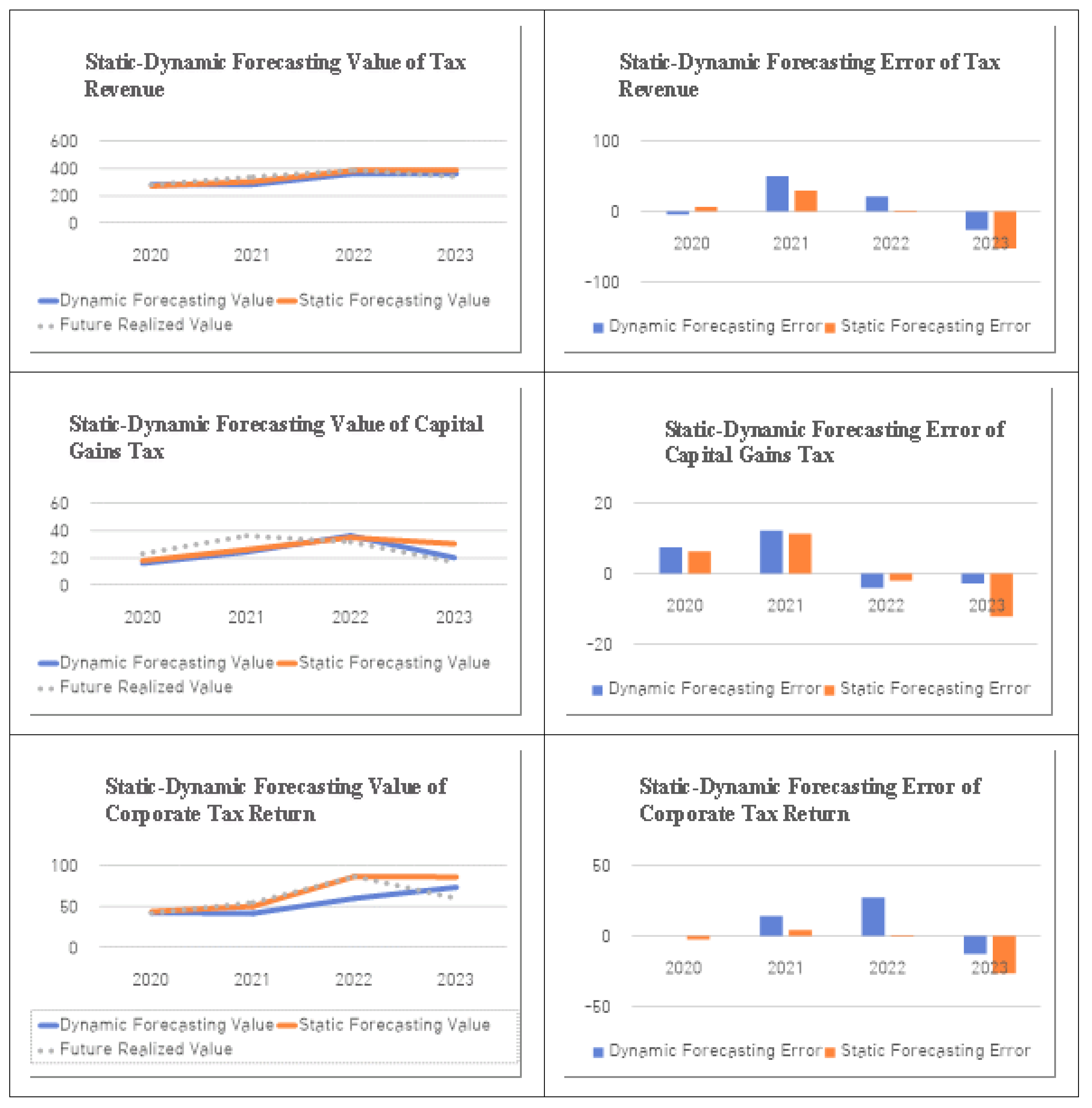

Table 1.
Forecasting Errors in Tax Revenue.
|
Average Error Rate (Trillion KRW) |
Mean Absolute Percentage Error (%) |
Autocorrelation of Errors (1.0) |
|
| National Tax | 2.016294 | 0.0452 | 0.14, -0.29, 0.04 |
| Income Tax | 2.209259 | 0.0571 | 0.17, -0.25, 0.10 |
| Labor Income Tax | 0.599985 | 0.0388 | - |
| Comprehensive Income Tax | 0.158278 | 0.0785 | - |
| Capital Gains Tax | 1.298696 | 0.2087 | - |
| Corporate Tax | -1.34889 | 0.0684 | -0.01, -0.26, 0.10 |
| Value Added Tax | 0.223954 | 0.0356 | 0.05, -0.05, 0.01 |
Table 2.
Results of Unit Root Tests.
| Variables Name | Level Variables | First Differenced Variables |
| National Tax | -1.630 | -4.812* |
| GDP | 0.146 | -4.451* |
| Domestic Assets | -2.362 | -2.534^ |
| Domestic Consumption | -3.430* | -3.896* |
| Wages | -1.392 | -4.765* |
| Number of Salaried Workers | -3.410* | -3.429* |
| Interest Income | -1.849 | -4.182* |
| Dividend Income | -2.190 | -6.314* |
| Business Income & Rental Income from Real Estate |
-3.816* | -2.915^ |
| Number of Non-Salaried Workers |
-0.307 | -4.240* |
| Transfer Price of Land | -1.782 | -4.472* |
| Transfer Price of Building | -2.441 | -4.922* |
| Transfer Price of Stocks | -0.356 | -3.231* |
| Transfer Price of Other Assets | -1.492 | -3.603* |
| Balance of Deposits & Bonds | -2.268 | -4.255* |
| Dividend on Stocks | -2.190 | -6.314* |
| Exchange Rate (Won-Dollar) | -1.680 | -4.221* |
| Short-term Interest Rate | -1.972 | -3.533* |
| Corporate Net Income | -2.656^ | -6.542* |
| Corporate Revenue | -0.946 | -4.178* |
| Capital Investment | -1.252 | -3.949* |
| Exports | -1.533 | -3.848* |
| Corporate Bond (3-year) Interest Rate |
-1.779 | -4.099* |
| Value of Inherited Assets | 1.086 | -4.702* |
| Value of Gifted Assets | -1.319 | -5.875* |
| Number of Decedents | -1.961 | -8.357* |
| Number of Gift Decisions | -1.318 | -8.080* |
| KOSPI Stocks | -1.835 | -4.760* |
| KOSDAQ Stocks | -0.633 | -5.808* |
| Other Stocks | -1.380 | -5.324* |
| Number of Stock Transactions | -1.924 | -5.326* |
| Stamp Duty Tax Payable | -1.584 | -4.100* |
| Issuance of stamped taxable documents |
-1.713 | -2.962^ |
| Individual property tax liability |
-1.264 | -3.168* |
| Corporate property tax liability |
-2.452 | -6.063* |
| Number of taxpayers for comprehensive real estate tax | -1.166 | -3.040^ |
| Business revenue | -1.077 | -3.668* |
| Imports | -1.765 | -4.227* |
| CPI | -1.760 | -2.646^ |
| Alcohol sales revenue | -1.121 | -3.791* |
| Alcohol Imports | -1.413 | -3.654* |
| Gasoline consumption | -1.497 | -4.732* |
| Diesel consumption | -0.679 | -3.721* |
| Sales of luxury taxed goods | -0.797 | -2.445 |
| Sales at taxable locations | -1.804 | -3.500* |
| Sales at taxable entertainment venues |
-1.279 | -3.443* |
| Effective tariff rate | 0.735 | -4.673* |
Note that each value represents the t-statistic. * and ^ indicate statistical significance at the 5% (critical value = -2.99 to -3.08) and 10% (critical value = -2.63 to -2.68) levels, respectively.
Table 3.
Results of Cointegration Tests.
| Models | Engle-Granger Test | Gregory-Hansen Test |
| National Tax Function | -4.720^ (1 lag) | -7.416* (2 lags) |
| Labor Income Tax Function | -3.596 (3 lags) | -5.739^ (0 lag) |
| Comprehensive Income Tax Function |
-3.856 (0 lag) | -8.067* (0 lag) |
| Capital Gains Tax Function | -5.724* (1 lag) | -7.101* (0 lag) |
| Interest & Dividend Income Tax Function |
-2.976 (1 lag) | -6.840* (1 lag) |
| Corporate Tax Function | -5.780^ (0 lag) | -8.169* (0 lag) |
| Inheritance & Gift Tax Function |
-3.748 (3 lags) | -6.653* (3 lags) |
| Securities Transaction Tax Function |
-2.474 (0 lag) | -8.740* (0 lag) |
| Stamp Duty Tax Function | -2.821 (0 lag) | -7.571* (3 lags) |
| Comprehensive Real Estate Tax Function |
-2.893 (0 lag) | -7.316* (5 lags) |
| Value-Added Tax Function | -3.314 (0 lag) | -6.022* (0 lag) |
| Liquor Tax Function | -4.799^ (1 lag) | -8.568* (5 lags) |
| Transportation, Energy, & Environmental Tax Function | -4.753* (0 lag) | -8.850* (0 lag) |
| Excise Tax Function | -3.158 (3 lags) | -7.473* (4 lags) |
| Tariff Function | -3.586 (1 lag) | -10.56* (5 lags) |
Each value represents the t-statistic. Asterisk (*) and caret (^) indicate statistical significance at the 5% level (critical values = -5.04 to -5.79 and -5.96 to -6.84) and the 10% level (critical values = -4.51 to -4.65), respectively, in the Engle-Granger and Gregory-Hansen tests, which account for structural changes.
Table 4.
Comparison of Forecasting Power for Labor Income Tax Revenue.
| Year | OLS | DOLS | FMLS | Government Forecast | Realized Values |
| 2022 | 47,454,983 | 73,080,548 | 48,682,097 | 61,255,200 | 60,370,406 |
| 2023 | 47,175,196 | 73,486,958 | 48,558,094 | 64,114,100 | 62,071,988 |
Unit of measurement = million KRW. DOLS and FMLS estimations selected leads/lags based on the AIC. Time-varying forecast values of explanatory variables in the in-sample tax revenue prediction model were forecasted using either actual values or predictions from the time series AR(1) model for convenience. Each value represents the estimated forecast of tax revenue.
Table 5.
Forecast for Labor Income Tax Revenue.
| Year | DOLS | FMLS | Random Simulation | Government Forecast |
| 2024 | 73,868,721 | 45,129,895 | 65,419,651 | - |
| 2025 | 74,227,332 | 45,036,277 | 74,432,574 | - |
Unit of measurement = million KRW. Time-varying forecast values of explanatory variables in the tax revenue prediction model were forecasted using predictions from the time series AR(1) model as a substitute for expert predictions. The dynamic model (DOLS) was based on forecasts derived from the DOLS lag model, while the single time series forecast was based on the AR(1) model. Each value represents the estimated forecast of tax revenue.
Table 6.
Comparison of Forecasting Power for Comprehensive Income Tax Revenue.
| Year | OLS | DOLS | FMLS | Government Forecast | Realized Values |
| 2022 | 20,247,079 | 40,278,892 | 13,784,847 | 23,706,600 | 26,011,631 |
| 2023 | 21,478,486 | 42,310.713 | 14,276,997 | 27,082,300 | 23,739,939 |
Unit of measurement = million KRW. DOLS and FMLS estimations selected leads/lags based on the AIC. Time-varying forecast values of explanatory variables in the in-sample tax revenue prediction model were forecasted using either actual values or predictions from the time series AR(1) model for convenience. Each value represents the estimated forecast of tax revenue.
Table 7.
Forecast for Comprehensive Income Tax Revenue.
| Year | DOLS | FMLS | Random Simulation | Government Forecast |
| 2024 | - | 15,899,180 | 24,438,323 | - |
| 2025 | - | 17,173,790 | 25,177,055 | - |
Unit of measurement = million KRW. Time-varying forecast values of explanatory variables in the tax revenue prediction model were forecasted using predictions from the time series AR(1) model as a substitute for expert predictions. The dynamic model (DOLS) was based on forecasts derived from the DOLS lag model, while the single time series forecast was based on the AR(1) model. Each value represents the estimated forecast of tax revenue.
Table 8.
Comparison of Forecasting Power for Capital Gains Tax Revenue.
| Year | OLS | DOLS | FMLS | Government Forecast | Realized Values |
| 2022 | 24,007,652 | - | 25,093,685 | 34,222,800 | 32,233,279 |
| 2023 | 21,428,994 | - | 22,316,145 | 29,719,700 | 17,556,007 |
Unit of measurement = million KRW. DOLS and FMLS estimations selected leads/lags based on the AIC. Time-varying forecast values of explanatory variables in the in-sample tax revenue prediction model were forecasted using either actual values or predictions from the time series AR(1) model for convenience. Each value represents the estimated forecast of tax revenue.
Table 9.
Forecast for Capital Gains Tax Revenue.
| Year | DOLS | FMLS | Random Simulation | Government Forecast |
| 2024 | - | 20,400,238 | 25,221,911 | - |
| 2025 | - | 19,081,552 | 20,551,933 | - |
Unit of measurement = million KRW. Time-varying forecast values of explanatory variables in the tax revenue prediction model were forecasted using predictions from the time series AR(1) model as a substitute for expert predictions. The dynamic model (DOLS) was based on forecasts derived from the DOLS lag model, while the single time series forecast was based on the AR(1) model. Each value represents the estimated forecast of tax revenue.
Table 10.
Comparison of Forecasting Power for Interest & Dividend Income Tax Revenue.
| Year | OLS | DOLS | FMLS | Government Forecast | Realized Values |
| 2022 | 6,296,667 | - | 8,263,376 | 6,996,000 | 6,785,436 |
| 2023 | 6,235,657 | - | 8,169,046 | 7,667,900 | 9,269,134 |
Unit of measurement = million KRW. DOLS and FMLS estimations selected leads/lags based on the AIC. Time-varying forecast values of explanatory variables in the in-sample tax revenue prediction model were forecasted using either actual values or predictions from the time series AR(1) model for convenience. Each value represents the estimated forecast of tax revenue.
Table 11.
Forecast for Interest and Dividend Income Tax Revenue.
| Year | DOLS | FMLS | Random Simulation | Government Forecast |
| 2024 | - | 8,087,387 | 10,348,028 | - |
| 2025 | - | 8,016,698 | 11,040,117 | - |
Unit of measurement = million KRW. Time-varying forecast values of explanatory variables in the tax revenue prediction model were forecasted using predictions from the time series AR(1) model as a substitute for expert predictions. The dynamic model (DOLS) was based on forecasts derived from the DOLS lag model, while the single time series forecast was based on the AR(1) model. Each value represents the estimated forecast of tax revenue.
Table 12.
Comparison of Forecasting Power for Corporate Tax Revenue.
| Year | OLS | DOLS | FMLS | Government Forecast | Realized Values |
| 2022 | 115,882,002 | 86,331,110 | 113,924,418 | 104,066,200 | 103,570,360 |
| 2023 | 110,741,642 | 78,011,548 | 108,111,567 | 104,996,900 | 80,419,515 |
Unit of measurement = million KRW. DOLS and FMLS estimations selected leads/lags based on the AIC. Time-varying forecast values of explanatory variables in the in-sample tax revenue prediction model were forecasted using either actual values or predictions from the time series AR(1) model for convenience. Each value represents the estimated forecast of tax revenue.
Table 13.
Forecast for Corporate Tax Revenue.
| Year | DOLS | FMLS | Random Simulation |
Government Forecast |
| 2024 | 79,805,321 | 117,995,029 | 87,459,557 | 77,700,000 |
| 2025 | 81,549,804 | 119,983,137 | 81,974,971 | - |
Unit of measurement = million KRW. Time-varying forecast values of explanatory variables in the tax revenue prediction model were forecasted using predictions from the time series AR(1) model as a substitute for expert predictions. The dynamic model (DOLS) was based on forecasts derived from the DOLS lag model, while the single time series forecast was based on the AR(1) model. Each value represents the estimated forecast of tax revenue.
Table 14.
Comparison of Forecasting Power for Inheritance & Gift Tax Revenue.
| Year | OLS | DOLS | FMLS | Government Forecast | Realized Values |
| 2022 | 14,565,350 | 12,951,035 | 10,526,439 | 15,903,600 | 14,594,019 |
| 2023 | 11,342,532 | 13,684,923 | 10,852,096 | 17,127,400 | 14,634,054 |
Unit of measurement = million KRW. DOLS and FMLS estimations selected leads/lags based on the AIC. Time-varying forecast values of explanatory variables in the in-sample tax revenue prediction model were forecasted using either actual values or predictions from the time series AR(1) model for convenience. Each value represents the estimated forecast of tax revenue.
Table 15.
Forecast for Inheritance & Gift Tax Revenue.
| Year | DOLS | FMLS | Random Simulation |
Government Forecast |
| 2024 | 14,438,605 | 12,822,476 | 15,938,336 | 14,700,000 |
| 2025 | 15,212,612 | 13,729,379 | 17,897,784 | - |
Unit of measurement = million KRW. Time-varying forecast values of explanatory variables in the tax revenue prediction model were forecasted using predictions from the time series AR(1) model as a substitute for expert predictions. The dynamic model (DOLS) was based on forecasts derived from the DOLS lag model, while the single time series forecast was based on the AR(1) model. Each value represents the estimated forecast of tax revenue.
Table 16.
Comparison of Forecasting Power for Securities Transaction Tax Revenue.
| Year | OLS | DOLS | FMLS | Government Forecast | Realized Values |
| 2022 | 7,075,899 | 6,084,432 | 5,869,009 | 7,538,000 | 6,302,867 |
| 2023 | 8,540,173 | 7,318,489 | 7,671,893 | 4,973,900 | 6,080,262 |
Unit of measurement = million KRW. DOLS and FMLS estimations selected leads/lags based on the AIC. Time-varying forecast values of explanatory variables in the in-sample tax revenue prediction model were forecasted using either actual values or predictions from the time series AR(1) model for convenience. Each value represents the estimated forecast of tax revenue.
Table 17.
Forecast for Securities Transaction Tax Revenue.
| Year | DOLS | FMLS | Random Simulation |
Government Forecast |
| 2024 | 6,766,729 | 6,842,655 | 4,823,444 | 5,400,000 |
| 2025 | 6,346,607 | 6,522,208 | 3,523,887 | - |
Unit of measurement = million KRW. Time-varying forecast values of explanatory variables in the tax revenue prediction model were forecasted using predictions from the time series AR(1) model as a substitute for expert predictions. The dynamic model (DOLS) was based on forecasts derived from the DOLS lag model, while the single time series forecast was based on the AR(1) model. Each value represents the estimated forecast of tax revenue.
Table 18.
Comparison of Forecasting Power for Stamp Duty Tax Revenue.
| Year | OLS | DOLS | FMLS | Government Forecast | Realized Values |
| 2022 | 739,322 | 933,881 | 778,234 | 948,000 | 798,775 |
| 2023 | 756,922 | 956,112 | 796,760 | 815,800 | 796,932 |
Unit of measurement = million KRW. DOLS and FMLS estimations selected leads/lags based on the AIC. Time-varying forecast values of explanatory variables in the in-sample tax revenue prediction model were forecasted using either actual values or predictions from the time series AR(1) model for convenience. Each value represents the estimated forecast of tax revenue.
Table 19.
Forecast for Stamp Duty Tax Revenue.
| Year | DOLS | FMLS | Random Simulation |
Government Forecast |
| 2024 | 953,683 | 794,736 | 696,338 | 900,000 |
| 2025 | 951,667 | 793,055 | 629,011 | - |
Unit of measurement = million KRW. Time-varying forecast values of explanatory variables in the tax revenue prediction model were forecasted using predictions from the time series AR(1) model as a substitute for expert predictions. The dynamic model (DOLS) was based on forecasts derived from the DOLS lag model, while the single time series forecast was based on the AR(1) model. Each value represents the estimated forecast of tax revenue.
Table 20.
Comparison of Forecasting Power for Comprehensive Real Estate Tax Revenue.
| Year | OLS | DOLS | FMLS | Government Forecast | Realized Values |
| 2022 | 4,978,436 | - | 4,116,194 | 8,620,400 | 6,798,810 |
| 2023 | 4,713,769 | - | 3,789,957 | 5,713,300 | 4,596,509 |
Unit of measurement = million KRW. DOLS and FMLS estimations selected leads/lags based on the AIC. Time-varying forecast values of explanatory variables in the in-sample tax revenue prediction model were forecasted using either actual values or predictions from the time series AR(1) model for convenience. Each value represents the estimated forecast of tax revenue.
Table 21.
Forecast for Comprehensive Real Estate Tax Revenue.
| Year | DOLS | FMLS | Random Simulation |
Government Forecast |
| 2024 | - | 4,054,696 | 4,849,347 | 4,100,000 |
| 2025 | - | 4,336,215 | 3,648,200 | - |
Unit of measurement = million KRW. Time-varying forecast values of explanatory variables in the tax revenue prediction model were forecasted using predictions from the time series AR(1) model as a substitute for expert predictions. The dynamic model (DOLS) was based on forecasts derived from the DOLS lag model, while the single time series forecast was based on the AR(1) model. Each value represents the estimated forecast of tax revenue.
Table 22.
Comparison of Forecasting Power for Value-Added Tax Revenue.
| Year | OLS | DOLS | FMLS | Government Forecast | Realized Values |
| 2022 | 81,872,915 | 73,718,715 | 82,226,998 | 79,323,300 | 81,626,608 |
| 2023 | 84,386,117 | 74,214,848 | 85,213,803 | 83,203,500 | 73,774,862 |
Unit of measurement = million KRW. DOLS and FMLS estimations selected leads/lags based on the AIC. Time-varying forecast values of explanatory variables in the in-sample tax revenue prediction model were forecasted using either actual values or predictions from the time series AR(1) model for convenience. Each value represents the estimated forecast of tax revenue.
Table 23.
Forecast for Value-Added Tax Revenue.
| Year | DOLS | FMLS | Random Simulation |
Government Forecast |
| 2024 | 77,330,783 | 88,386,792 | 72,961,110 | 81,400,000 |
| 2025 | 80,494,634 | 88,170,229 | 76,822,040 | - |
Unit of measurement = million KRW. Time-varying forecast values of explanatory variables in the tax revenue prediction model were forecasted using predictions from the time series AR(1) model as a substitute for expert predictions. The dynamic model (DOLS) was based on forecasts derived from the DOLS lag model, while the single time series forecast was based on the AR(1) model. Each value represents the estimated forecast of tax revenue.
Table 24.
Comparison of Forecasting Power for Liquor Tax Revenue.
| Year | OLS | DOLS | FMLS | Government Forecast | Realized Values |
| 2022 | 3,330,650 | 4,344,958 | 3,569,676 | 3,737,400 | 3,766,531 |
| 2023 | 3,619,343 | 4,370,925 | 3,950,186 | 3,215,100 | 3,568,637 |
Unit of measurement = million KRW. DOLS and FMLS estimations selected leads/lags based on the AIC. Time-varying forecast values of explanatory variables in the in-sample tax revenue prediction model were forecasted using either actual values or predictions from the time series AR(1) model for convenience. Each value represents the estimated forecast of tax revenue.
Table 25.
Forecast for Liquor Tax Revenue.
| Year | DOLS | FMLS | Random Simulation |
Government Forecast |
| 2024 | 4,393,914 | 3,581,606 | 3,387,817 | 3,600,000 |
| 2025 | 4,414,268 | 3,599,901 | 3,594,276 | - |
Unit of measurement = million KRW. Time-varying forecast values of explanatory variables in the tax revenue prediction model were forecasted using predictions from the time series AR(1) model as a substitute for expert predictions. The dynamic model (DOLS) was based on forecasts derived from the DOLS lag model, while the single time series forecast was based on the AR(1) model. Each value represents the estimated forecast of tax revenue.
Table 26.
Comparison of Forecasting Power for Transportation, Energy, and Environmental Tax Revenue.
Table 26.
Comparison of Forecasting Power for Transportation, Energy, and Environmental Tax Revenue.
|
Year |
OLS | DOLS | FMLS | Government Forecast | Realized Values |
| 2022 | 14,926,271 | 10,820,812 | 14,737,361 | 10,902,200 | 11,116,375 |
| 2023 | 14,531,197 | 10,821,555 | 14,371,551 | 11,147,100 | 10,843,590 |
Unit of measurement = million KRW. DOLS and FMLS estimations selected leads/lags based on the AIC. Time-varying forecast values of explanatory variables in the in-sample tax revenue prediction model were forecasted using either actual values or predictions from the time series AR(1) model for convenience. Each value represents the estimated forecast of tax revenue.
Table 27.
Forecast for Transportation, Energy, and Environmental Tax Revenue.
| Year | DOLS | FMLS | Random Simulation |
Government Forecast |
| 2024 | 10,866,490 | 14,634,396 | 8,648,887 | 15,300,000 |
| 2025 | 10,908,554 | 14,669,421 | 12,792,677 | - |
Unit of measurement = million KRW. Time-varying forecast values of explanatory variables in the tax revenue prediction model were forecasted using predictions from the time series AR(1) model as a substitute for expert predictions. The dynamic model (DOLS) was based on forecasts derived from the DOLS lag model, while the single time series forecast was based on the AR(1) model. Each value represents the estimated forecast of tax revenue.
Table 28.
Comparison of Forecasting Power for Excise Tax Revenue.
| Year | OLS | DOLS | FMLS | Government Forecast | Realized Values |
| 2022 | 10,366,284 | 11,150,489 | 10,386,234 | 10,141,800 | 9,318,244 |
| 2023 | 9,982,999 | 11,716,815 | 9,879,189 | 10,194,300 | 8,820,924 |
Unit of measurement = million KRW. DOLS and FMLS estimations selected leads/lags based on the AIC. Time-varying forecast values of explanatory variables in the in-sample tax revenue prediction model were forecasted using either actual values or predictions from the time series AR(1) model for convenience. Each value represents the estimated forecast of tax revenue.
Table 29.
Forecast for Excise Tax Revenue.
| Year | DOLS | FMLS | Random Simulation |
Government Forecast |
| 2024 | 11,385,895 | 10,710,858 | 9,218,981 | 10,200,000 |
| 2025 | 11,773,296 | 11,006,891 | 8,805,095 | - |
Unit of measurement = million KRW. Time-varying forecast values of explanatory variables in the tax revenue prediction model were forecasted using predictions from the time series AR(1) model as a substitute for expert predictions. The dynamic model (DOLS) was based on forecasts derived from the DOLS lag model, while the single time series forecast was based on the AR(1) model. Each value represents the estimated forecast of tax revenue.
Table 30.
Comparison of Forecasting Power for Tariff Revenue.
| Year | OLS | DOLS | FMLS | Government Forecast | Realized Values |
| 2022 | 9,166,752 | - | 9,269,158 | 10,061,300 | 10,324,100 |
| 2023 | 8,744,282 | - | 8,944,291 | 10,723,700 | 7,288,300 |
Unit of measurement = million KRW. DOLS and FMLS estimations selected leads/lags based on the AIC. Time-varying forecast values of explanatory variables in the in-sample tax revenue prediction model were forecasted using either actual values or predictions from the time series AR(1) model for convenience. Each value represents the estimated forecast of tax revenue.
Table 31.
Forecast for Tariff Revenue.
| Year | DOLS | FMLS | Random Simulation |
Government Forecast |
| 2024 | - | 9,088,959 | 6,972,267 | 8,900,000 |
| 2025 | - | 8,776,880 | 5,946,109 | - |
Unit of measurement = million KRW. Time-varying forecast values of explanatory variables in the tax revenue prediction model were forecasted using predictions from the time series AR(1) model as a substitute for expert predictions. The dynamic model (DOLS) was based on forecasts derived from the DOLS lag model, while the single time series forecast was based on the AR(1) model. Each value represents the estimated forecast of tax revenue.
Table 32.
National Tax Revenue Forecast.
| Year |
Government Budget Tax Revenue |
Cointegration Model Predicted Tax Revenue |
Actual Settled Tax Revenue |
| 2022 | 373,516,400 | 338,248,056 | 372,597,472 |
| 2023 | 374,763,900 | 329,660,892 | 322,355,548 |
| 2024 | 378,420,800 | 335,694,309 | 324,000,000* |
| 2025 | - | 341,524,525 | - |
The actual settled tax revenue was measured in millions of KRW. For convenience, national tax was calculated as total revenue minus education tax, rural development tax, and other income taxes. * indicates the predicted value. For the 2024 fiscal year, values for other income taxes, education tax, and rural development tax were based on the 2023 figures. Specifically, the 2024 budgeted and settled amounts for other income taxes, education tax, and rural development tax used the same values as those from 2023.
Disclaimer/Publisher’s Note: The statements, opinions and data contained in all publications are solely those of the individual author(s) and contributor(s) and not of MDPI and/or the editor(s). MDPI and/or the editor(s) disclaim responsibility for any injury to people or property resulting from any ideas, methods, instructions or products referred to in the content. |
© 2025 by the authors. Licensee MDPI, Basel, Switzerland. This article is an open access article distributed under the terms and conditions of the Creative Commons Attribution (CC BY) license (http://creativecommons.org/licenses/by/4.0/).
Copyright: This open access article is published under a Creative Commons CC BY 4.0 license, which permit the free download, distribution, and reuse, provided that the author and preprint are cited in any reuse.


