
Submitted:
01 July 2025
Posted:
03 July 2025
You are already at the latest version
Abstract
Multimodal optimization is to find multiple global and local optimal solutions of a function, rather than a single solution. This study proposes a harmony search algorithm with iterative optimizing operators to solve the NP-hard distributed permutation flowshop scheduling for multimodal optimization. First, the initial solution set is constructed by using a distributed NEH operator. Second, after generating new candidate solutions, efficient iterative optimizing operators are applied to optimize these solutions and the worst solutions in the harmony memory(HM) are replaced. The proposed operations are repeated until the stopping condition of the algorithm is met. Finally, the solutions satisfying multimodal optimization in the harmony memory are obtained. The constructed method is compared with two meta-heuristics, the iterative greedy meta-heuristic algorithm with a bounded search strategy and the improved Jaya algorithm, on 600 newly generated datasets. The results show that it runs stably and outperforms the two algorithms compared.
Keywords:
distributed permutation flowshop
; harmony search
; iterative optimizing operator
; multimodal optimization
; makespan
I. Introduction
Compared to the single workshop’s processing mode of traditional manufacturing system, the distributed manufacturing system (DMS) fully utilizes the resources in the workshops of distributed factories. By realizing effective allocation of raw materials, optimal combination of productivity, scientific and reasonable resource sharing etc., the goal of quickly achieving product manufacturing at reasonable costs in DMS is fulfilled.
Distributed scheduling plays a crucial role in DMS, it has the characteristics of large-scale, nonlinear, strong constraints, multi-objective, uncertainty, and has always been a hot topic in the fields of optimization and manufacturing. Its scientific optimization directly affects the efficiency and long-term development of production enterprises. Therefore, developing efficient optimization scheduling algorithms is one of the keys for improving the production efficiency, saving energy, reducing emissions, decreasing production costs, and solving the bottleneck problem.
In DMS, the distributed flowshop scheduling problem (DFSP) is a very important problem. Due to the presence of multiple factories, the DFSP encounters many challenges, such as the coupling relationship between processing factories, allocation of machines within the factory, and sorting of jobs to be processed [1]. Compared with the traditional NP-hard flowshop scheduling problem in a single factory, the DFSP has a larger solution space, and involves greater difficulty in arriving at the optimal solution. It imposes more stringent requirements on the accuracy and speed of the algorithm. Therefore, research on the problem has theoretical and applicative importance.
Many researchers have proposed various algorithms for solving the DFSP in different scenarios and under different constraints by focusing on different objectives of multimodal optimization. Li and Wu [2] proposed Heuristic for no-wait flow shops with makespan minimization based on total idle-time increments. Gogos [3] addressed the DFSP by using constraint programming and its special scheduling features for makespan minimization. Hao, Li, Du, Song, Duan and Zhang [4] studied the distributed hybrid flowshop scheduling (DHFS) problem for makespan minimization and established a mathematical model. Geng and Li [5] studied an improved hyperplane-assisted evolutionary algorithm to solve a distributed mixed flowshop scheduling problem in a glass manufacturing system with two objectives: minimizing makespan and the total energy consumption. Zhang and Geng et al. [6] proposed an effective Q-learning-based multi-objective particle swarm optimization algorithm to solve the DFSP problem, with the total completion time and total energy consumption minimization. Bai and Liu et al. [7] studied a heterogeneous distributed permutation flowshop scheduling problem to minimize the makespan. Zhao, Zhuang, Wang and Dong [8] investigated the distributed no-idle permutation flowshop scheduling problem (DNIPFSP). The makespan and total tardiness are optimized simultaneously considering the variety of scales of the problems with introducing an improved iterative greedy (IIG) algorithm. Li, Pan, Sang, Jing, Framiñán and Li [9] addressed a distributed permutation flowshop scheduling problem with part of jobs subject to a common deadline, established a mathematical model and proposed a self-adaptive population-based iterated greedy algorithm with the objective of minimizing the total completion time. Song, Lin and Chen [10] studied the distributed assembly permutation flowshop scheduling problem with sequence dependent setup times. An effective two-stage heuristic was proposed with the optimization objective of minimizing makespan.
The harmony search (HS) algorithm, proposed by Geem, Kim, and Loganathan [11], is a simple but effective meta-heuristic. It is based on the processes involved in musical performance when a composer searches for a better musical harmony, such as during jazz improvisation. Jazz improvisation seeks to find musically pleasing harmonies as determined by an aesthetic standard, just as the process of optimization seeks to find a global optimal solution as determined by an objective function. The pitch of each musical instrument determines the overall aesthetic quality, just as the value of the objective function is determined by the set of values assigned to each decision variable. HS has been widely applied to various optimization problems in science and engineering, including tour planning, Internet routing, and the design of water networks and hearing aids [12].
The distributed permutation flowshop scheduling problem(DPFSP) is considered in this study, as it is one of the most widely studied problems in the field of scheduling. Because HS is a simple but effective meta-heuristic, a hybrid algorithm based on HS is proposed to solve this problem for multimodal optimization with its objective of makespan minimization.
The remaining part of this paper is organized as follows: Section II provides an objective of minimizing makespan and a mathematical model for the considered problem. Combined with iterative optimization algorithms, Section III presents a hybrid harmony search algorithm, named IOHS. Section IV conducts simulation experiments based on experimental data to verify the effectiveness of the algorithm, and compares its performance with other algorithms. Section V provides conclusions and prospects for future research contents and directions.
II. Problem Description
The DPFSP can be described as follows: assume that a batch of sequentially numbered jobs are first assigned to some distributed homogeneous factories, and then, the jobs in each factory are scheduled and processed sequentially on the machines. The goal is to provide the (approximately) optimal job–factory allocation and sequence of jobs within the factory for multimodal optimization.
The main assumptions are as follows:
- All jobs are ready when processing starts.
- The number of jobs and their processing times on machines are known, and are non-negative.
- Each job can be processed only on one machine in a given factory at a given time, and cannot be pre-empted.
- Each machine can process only one job at a time, and completes all jobs in sequence.
- The preparation time for each job is sequence independent, and is included in its processing time.
The symbols and definitions used in this paper are as follows:
F: Number of factories.
f: Index for factories, .
M: Number of machines in each factory.
m: Index for machines, .
: Number of jobs in factory f.
J: Total number of jobs, .
: The n-th job assigned to factory f, .
: The processing time of the n-th job in factory f on machine m.
A solution can then be given by Equation (1):
Equation (1) shows that is composed of two parts: The first part shows the number of jobs assigned to each factory while the second part displays the sequence of jobs processed in each factory.
The formulae for calculating the completion time of each job on the machines in the factory are given by Equations (2)–(5):
Equation (2) shows the completion time of the first job on the first machine in each factory. This is the processing time for this job on the given machine. Equation (3) shows the completion time of the first job on the m-th machine in each factory, and this is the sum of the processing times of the job from the first machine to the m-th machine. Equation (4) shows the completion time of the n-th job on the first machine in each factory. This is the sum of processing times of the previous n jobs on the first machine. Equation (5) shows the completion time of the n-th job on the m-th machine in each factory. This is the sum of processing times of job on the m-th machine, and is the maximum value of the completion time of job on the (m-1)-th machine, or the completion time of job on the m-th machine:
The makespan of factory f is the completion time of the last job on the last machine and is shown in Equation (6). The makespan for collaborative processing in DMS is the maximum value among and is shown in Equation (7).
The solution in the solution space that has the minimum makespan, can be depicted by Equation (8):
Based on the above analysis and formulae, the aim of this paper is to propose an algorithm to find multiple global and local optima of a function, thus the user can have a better knowledge about different optimal solutions in the search space and when needed, the current solution may be switched to a more suitable one while still maintaining the optimal system performance [13].
III. Proposed Algorithm
A. Harmony Search Algorithm
The basic process for HS is shown in Algorithm 1.
| Algorithm 1. Harmony search algorithm(HS) |
| Initialize parameters , , , ; For (i =1 to ){ Select values within the range of the decision variable to generate a harmony solution; Put the solution into HM; } Repeat Set ; For ( i =1 to n ){ Generate a random number ; If ( ){ Select a value as the i-th decision variable of from the historical solution of HM; Generate a random number ; If( ) Adjust this decision variable according to the adjustment bandwidth bw to obtain a new decision variable; }Else{ Select a value as the i-th decision variable of within the range of values of the decision variable; } } According to the objective function, find the worst solution in HM; If ( is better than Replace with ; Until (the stopping condition is satisfied); Return; |
In HS algorithm, is the rate of consideration of HM, and is the probability of taking a value from HM. is the rate of pitch adjustment, and is the probability of adjusting a value. is the size of HM, bw is the bandwidth of adjustment. and are two random numbers in range (0, 1). The algorithm consists of three main parts: (1) initialization of HM, (2) generation of a new solution, (3) update of HM.
(1) Initialization of HM
The initialization of HM is used to generate the initial solution set, and is the first stage of this evolutionary computing algorithm. In HS algorithm, the initial solution set of HM is randomly generated. In other words, harmony solutions are randomly generated from the solution space with n variables, and are placed in HM. The form of HM is given in Equation (9):
(2) Generation of a New Solution
It involves two stages to generate a new solution: the construction stage and the adjustment stage. In the construction stage, a random number is generated and compared with . If is smaller than , a harmony variable is selected from HM, otherwise, a harmony variable is generated from the solution space. For each harmony variable obtained from HM, another random number is generated in the adjustment stage and compared with . If is smaller than , the variable needs to be adjusted according to the adjustment bandwidth bw to obtain a new value. Otherwise, no adjustment is carried out. By performing this process n times, a new harmony is obtained.
(3) Update of HM
The new generated solution is evaluated based on the objective function of optimization. If is better than the worst solution in HM, then the solution is replaced by the new solution , otherwise, there is no update.
B. Harmony Search with Iterative Optimization
HS algorithm was originally developed for continuous functions of n variables, and it has the essence of continuity [11]. However the problem studied here involves decision variables with discrete characteristics. Therefore, a hybrid HS algorithm is proposed by modifying HS algorithm suitable for solving the considered problem.
(1) Initialization of HM
Due to the homogeneity of DMS, whereby all factories have the same number and sequence of machines with identical characteristics of processing, there is no need to optimize the order of factories, and they can be arranged in numerical order. Each solution in HM consists of two parts: The first part stores the number of jobs allocated by each factory in order, which displays the structure of the solution. The second part deals with the jobs and their arrangement within a given factory. Assigning different numbers of jobs to a factory and scheduling them can significantly influence the makespan of that factory. The two factors, job–factory allocation, and job ordering within that factory, thus influence the objectives of scheduling. These factors cannot be simply separated, and need to be studied as a whole.
Assuming that there are 9 sequentially numbered jobs assigned to 3 distributed manufacturing factories, Table 1 shows an example of a HM. This example contains two harmony solutions represented as and respectively. For the second solution ={{4,2,3}|{1,3,4,9},{2,5},{6, 7,8}}, the first part of the solution {4,2,3} indicates that there are 3 processing factories, and there are 4 jobs in the first factory,2 jobs in the second one and 3 jobs in the third one. The second part shows in detail that the first 4 jobs {1,3,4,9} are assigned to the first factory, the next 2 jobs {2,5} are assigned to the second one, and the last 3 jobs {6,7,8} are assigned to the third one.
The quality of the initial solution set is important for the evolution of the algorithm because it determines whether the algorithm can quickly find the (approximately) optimal solution or not. The NEH algorithm [14] is an efficient and widely used heuristic algorithm to obtain an initial solution for scheduling problems with makespan minimization. Its main idea is as follows: First, arrange the n jobs in descending order according to the processing times on machines of each job. Second, pick the first two jobs from the list and find the best sequence for these two jobs by calculating makespan for the two possible sequences, set i=2. Third, pick the job in the (i+1)-th position of the list and find the best sequence by placing it at all possible (i+1) positions in the partial sequence found previously. Repeat the third step till i=n.
However, the problem considered in this paper is distributed permutation flowshop scheduling with multiple factories, the NEH algorithm cannot be directly used to obtain the initial solution set. Thus a distributed NEH algorithm (D-NEH) is constructed to obtain the initial solution set. It can be obtained by the following procedure: First, generate a job sequence by arranging the J jobs in descending order according to their processing times on the machines, and randomly generate the other job sequences. Then, for each of the job sequences, assign the first F jobs to F factories (each factory contains one job), pick the next job from the job sequence, and find the best position by placing it in all possible positions in the partial sequence of each factory, repeat the pick–find operation until all the jobs have been arranged to its proper factory and the best position in that factory. Finally, the initial solution set HM is generated.
The D-NEH algorithm for initial solution generation is shown in Algorithm 2.
| Algorithm 2. D-NEH algorithm |
| Initialize the parameter
; Generate the first job sequence by arranging the J jobs in descending order according to their processing times on the machines; Randomly generate the other job sequences; For (i = 1 to ){ Assign the first F jobs to F factories; For(j=F; j<J; j++){ Pick the job in the (j+1)-th position of the job sequence Find the best sequence by placing it in all possible positions in the partial sequence of each factory; } } Return; |
(2) Generation of New Solution
The process of generating new solutions can be divided into three stages. The first two stages are identical to those in HS algorithm, while the third one is an optimization stage. Unlike the case in which there is one solution sequence for only one factory, a DMS in the construction stage has at least two factories, each of which may not necessarily contain the same number of jobs. Therefore, before constructing a new solution sequence, the number of different solution structures contained in HM should first be obtained. Then, based on the number of jobs in each factory in the solution structure, if the random number is smaller than the parameter , a new solution is constructed by selecting jobs from HM, otherwise, the solution is constructed by selecting jobs from a range of possible values for each decision variable. It is clear that, in the stage of construction of the new solution, solutions are generated instead of one. The construction stage essentially combines the architecture of certain meta-heuristic algorithms. For example, it preserves the historical traces of past vectors, similarly to the taboo search algorithm [15]. It can have a varying probability of fitness from the beginning to the end of the calculation, similarly to the simulated annealing algorithm [16]. At the same time, it can retain several vectors like genetic algorithms to enable the newly generated solution to evolve.
The adjustment stage in this algorithm involves a certain variation based on the parameter while the solution is obtained by considering convergence and divergence in the generation of the new solution by the algorithm. That is, the algorithm constructs the solution while performing mutation on each decision variable by relying on . The main idea of this adjustment operation is that when it is executed, a decision variable is selected from the current solution sequence and exchanged with a randomly selected decision variable that is close to it. The solution with the best value of the objective function is used as the new solution. This idea is similar to that of the genetic algorithm, which creates a small random disturbance to avoid premature convergence.
In the optimization stage, an iterative optimization algorithm (IOA) which is composed of RZ and PE operators [2] is used to further search the neighborhood of the candidate solution to find more and better solutions. RZ and PE algorithms are commonly used and relatively efficient among heuristic algorithms. The main idea of RZ algorithm is as follows: For a given job sequence with n jobs, select a job from the sequence and insert it into n possible positions to find the best sequence, Repeat this select-insert operation for the next job in the job sequence until all of the jobs be selected/optimized. The main idea of PE algorithm is as follows: For a given job sequence with n jobs, pick a job from it and exchange this job with other n-1 jobs to find the best sequence, Repeat this pair-wise exchange operation for the next unpicked job until all of the jobs be picked/optimized.
The IOA operator can be described as follows: For each new candidate solution , select one job from the sequence with the largest makespan value (if there is more than one sequences, select one randomly) and insert it into other possible positions to find the best sequence . For , pick this job and exchange it with other jobs to find the best sequence . Repeat the select–insert and pairwise-exchange operations for the next unselected job until all the jobs have been optimized; at this point, the (approximately) optimal solution has been finally obtained. The IOA operator used to optimize a new candidate solution is presented in Algorithm 3.
| Algorithm 3. Iterative optimization algorithm (IOA) |
| Set
; Repeat Find the factory with the largest value of makespan in and record it as ; Set global false; For (j=1 to ){ For (f =1 to F){ If ( f = ) continue; Insert job j into factory f; Apply the select–insert operation to optimize the job sequence of factory f and get the best sequence ; Apply the pairwise exchange operation to further optimize the job sequence of factory f and get the best solution ; If( < ){ Replace with ; Set global true; } If (global=true) break; } If (global=true) break; } Until global=false; Set ; Return; |
After the construction and adjustment stages as well as the optimization of the candidate solution, new candidate solutions are generated, and are sorted in descending order according to the value of the objective function to facilitate the subsequent update of HM.
The proposed algorithm to generate and optimize new solutions is detailed in Algorithm 4.
| Algorithm 4. New solution generation algorithm (NSGA) |
| Initialize parameters ,,
; Set ; Obtain the total number of solution structures of HM; For (i =1 to ){ Let the i-th solution structure be the structure of the new solution ; Set ; For (j=1 to J ){ Generate two random numbers and ; If ( ){ Select a new job from column in HM and insert it into the j-th position of the new solution ; }Else{ Select a new job from the job set and insert it into the j-th position of the new solution ; } If ( ){ Adjust the job to within the range (max{0, j- bw}, min{ j+bw, J} ); } } Applying the IOA operator to optimize the new solution ; Set ; } Sort the new candidate solutions in descending order according to values of the objective function, and obtain the new solution set { }; Return; |
In the NSGA algorithm, the IOA operator is used to further optimize the candidate solutions for better ones. This not only increases the diversity of solutions in HM, but also enables the algorithm to expand the search space, and find more and better solutions. Therefore, this algorithm has a good ability to search the solution space and find more (approximately) optimal solutions while maintaining their diversity.
(3) Update of HM
The update operation enables the algorithm to obtain more and better solutions, which can guide it to search for a better solution space and accelerate the convergence of the solution. Therefore, the update operation plays an important role in maintaining high-quality solutions and ensuring the convergence of the algorithm.
According to the objective function, the main idea of the update operation is as follows: For each new generated harmony solution and the worst harmony solution found in HM, if is worse than , then replace with .
The update algorithm is detailed in Algorithm 5.
| Algorithm 5. Update algorithm |
| For (i =1 to t) { Set pos -1;-1; For (h =1 to ){ If ( { Set pos h, ; } } If ( and { Replace with ; } } Return; |
(4) Algorithm Description
The algorithm proposed in this paper is a hybrid meta-heuristic based on HS and iterative optimization, called IOHS. Following the generation of the initial solution set, the NSGA algorithm is used in this algorithm to construct new solutions. While constructing a new solution, it may select a new job from HM or a job set based on the parameter , and adjusts it to avoid local convergence based on the parameter . The IOA operator is used to further optimize the quality of the new solution and obtain the final candidate solution. The worst solutions in HM are replaced if they are poorer than the candidate solutions. The construction, optimization, and update operations are repeated until the algorithm satisfies its stopping condition. And finally, the solutions that satisfying the multimodal optimization are output.
IOHS algorithm is shown in Algorithm 6.
| Algorithm 6. IOHS algorithm |
| Generate the initial solution set of HM by using D-NEH; Repeat Construct a new solution set by using the NSGA algorithm; Use the Update algorithm to update HM; Until (the stopping condition is satisfied) Calculate the objective function values based on Equation (7); Output the solutions satisfying multimodal optimization based on Equation (8); Return; |
IV. Simulations
In this section, the test dataset used to assess the performance of the proposed method is first described. Then Statgraphics is used to analyze the parameters and , and finally the simulations are detailed. All the algorithms were coded in Java and executed on a Windows PC with an Intel® i5 core, 2.5 GHz CPU, and 4 GB RAM.
A. Test Dataset
The Taillard benchmark [17] has been widely used in scenarios involving single and multiple manufacturing factories. However, when the number of factories increases in the application of a distributed manufacturing system, the average number of jobs assigned to each factory may be very small. For example, if there exists a DMS consisting of 10 factories and 200 jobs, the average job allocation for each factory is only 10. Although the solution space is huge, the size of the problem for each factory is relatively small. Therefore, to faithfully simulate job allocation in distributed scenarios, a new dataset is generated which is based on the main idea of the data generation algorithm developed by Taillard.
The stopping condition of the algorithm is described in Section 5.2. The generated dataset was as follows: The processing time of each job on machines was randomly generated in the interval [5, 99]. The numbers of jobs J were set to 60, 150, 330, 510, and 600. The numbers of factories F were set to 2, 3, 5, and 10, respectively. The numbers of machines in each factory were set to 5, 10, and 20, respectively.
B. Parameter Analysis
The parameter represents the size of HM, i.e., the number of solutions in HM. Based on the total number of jobs to be sorted, is set to 0.2 × J. The parameter is used to increase the range of the search space, prevent the algorithm from prematurely converging, and improve the probability of finding a better solution. In this paper, is set as . To evaluate the algorithm fairly based on the number of machines and the average number of jobs per factory, the runtime of all the algorithms considered here are set as ms [18], where is the number of machines in each factory, J is the total number of jobs to be processed, F is the number of factories, and was set to 120.
The rates of consideration and pitch adjustment are two important parameters in HS algorithm. determines the probability of randomly generating a solution based on the historical variables in HM. As HM stores the best solutions obtained by the algorithm at any given time, the algorithm tends to find more optimized solutions (leading to faster convergence) when the value of increases. determines the probability of adjusting the values selected from among the historical values in HM, which means that it determines the probability of adjusting some vectors of a solution (probability of divergence). As the value of increases, the algorithm tends to generate solutions by selecting from global variables, that is, by expanding the search range (divergence) to find more optimized solutions. To determine appropriate values of and , they were tested with different values: was set to 0.70, 0.75, 0.80, 0.85, 0.90, and 0.95, while was set to 0.10, 0.15, 0.20, 0.25, 0.30, and 0.35. To test the parameter values fairly and quickly, M is set to 10, J to 330, and F to 5. For each parametric combination, a total of 20 instances were generated, each of which was executed three times, and the minimum value of the objective function was obtained. The average values of each parameter combination are shown in Table 2.
The analysis of the parameter combinations listed in Table 2 yielded the results shown in Figure 1, Figure 2 and Figure 3.
Figure 1 shows the results of a multivariate analysis of variance. As the value of increased and that of decreased, the solution obtained by the algorithm improved. This indicates that the larger the value of was and the smaller the value of was, the better was the performance of the algorithm. It is clear from Figure 2 that when =0.95 and =0.1, the algorithm obtained the best solution.
Figure 2 shows the results of a one-way analysis of variance for . Clearly, as the value of increased, the solution obtained by the algorithm improved. When was 0.95, the algorithm achieved the best solution.
Figure 3 shows the results of a one-way analysis of variance for , from which it is clear that as the value of decreased, the solution obtained by the algorithm improved. When was 0.1, the algorithm obtained the best solution.
It can be concluded that setting and can enable IOHS algorithm to obtain the best value of makespan.
C. Experimental Verification
(1) Comparison of HS and IOHS
HS and IOHS algorithm are compared from three perspectives, i.e., job, factory and machine, to show whether the optimization operator (named IOA) of IOHS algorithm gives the most contribution or not. The average makespan obtained by HS and IOHS algorithms are shown in Table 3.
Similarly, by conducting parameter analysis on the data in the Table 3, the following results can be drawn which are shown from Figure 4, Figure 5 and Figure 6.
Seen from Figure 4, it is obvious that as the number of jobs increases, the objective value obtained by the algorithm becomes larger and larger. Under the same number of jobs, IOHS algorithm outperforms HS algorithm.
Figure 5 shows that, as the number of factories increases, the number of jobs in each factory becomes smaller resulting in the fact that the objective value obtained by the algorithm becomes smaller and smaller. Under the same number of factories, IOHS algorithm outperforms HS algorithm.
Seen from Figure 6, it is obvious that as the number of machines increases, the objective value obtained by the algorithm becomes larger and larger. Under the same number of machines, IOHS algorithm outperforms HS algorithm.
In conclusion, IOHS algorithm is better than HS algorithm by using the optimization operator, thus the IOA operator gives a remarkable contribution to IOHS algorithm.
(2) Algorithms comparison
Many effective meta-heuristic algorithms have been developed in research, including PSO [19], DE [20], and CMA-ES [21], that can be compared with the proposed IOHS algorithm in the context of the DPFSP. However, only the iterative greedy meta-heuristic algorithm with a bounded search strategy(BSIG) [22] and the improved Jaya algorithm(Jaya)[23] are suitable for solving the problem considered here. They are implemented along with the proposed algorithm on a new dataset, with the aim of multimodal optimization. BSIG and the improved Jaya algorithms used the stopping condition described in Section 5.2. The average values of makespan obtained by these algorithms are shown in Table 4.
Table 4 shows that IOHS algorithm obtained the best results. For further analysis, the performance of these algorithms based on the average relative percentage deviation (ARPD) are compared, as defined in Equation (10):
Table 5 shows that BSIG algorithm delivered the worst performance, and that IOHS algorithm was slightly better than Jaya algorithm. To facilitate comparison, and visually display the trends of the solutions to the DPFSP obtained by different algorithms at different scales, the results of the multi-factor ANOVA are shown from Figure 7, Figure 8, Figure 9.
Figure 7 shows that as the number of jobs increased, the values of the objective function obtained by IOHS and Jaya algorithms both slightly increased, while the values obtained by BSIG algorithm decreased. This is because as the number of jobs increased, BSIG algorithm expanded its search range and found better solutions. However, owing to its significant randomness in searching for the (approximately) optimal solution, BSIG algorithm still delivered the worst results. It is clear that IOHS algorithm delivered the best performance of the three algorithms, regardless of the number of jobs.
Figure 8 shows that as the number of factories increased, the values of the objective function obtained by IOHS and Jaya algorithms both exhibited a downward trend, while those obtained by BSIG algorithm fluctuated. This is because as the number of factories increased, the number of jobs per factory decreased, and this enabled IOHS and Jaya algorithms to find better solutions. It is clear that IOHS algorithm delivered the best performance of the three algorithms, regardless of the number of factories.
Figure 9 shows that as the number of machines increased, the values of the objective function obtained by all three algorithms exhibited a decreasing trend. This is because the processing time for each job increased with the number of machines. It is clear that IOHS algorithm delivered the best performance of the three algorithms, regardless of the number of machines.
- Although the ARPD values obtained by BSIG algorithm fluctuated, they generally showed a downward trend. The ARPD values obtained by Jaya and IOHS algorithms both slightly decreased.
- Jaya algorithm was superior to BSIG algorithm, while the results obtained by IOHS algorithm were slightly better than those of Jaya algorithm.
- The results obtained by IOHS algorithm, shown in Table 5 and the corresponding figures, reveal that it delivered the best and most stable performance in solving the DPFSPs at all scales.
In summary, the proposed IOHS algorithm is an efficient and effective method, and it should be used to solve DPFSPs.
V. Conclusion
This study analyzed distributed permutation flowshop scheduling, provided a detailed description of the problem, and proposed a hybrid harmony search for multimodal optimization. The proposed algorithm initializes HM, continuously constructs and adjusts new solutions while optimizing them, and updates HM until the stopping condition is met. A comparison between this method, and two classic and recently developed algorithms showed that it is suitable for solving DPFSPs.
The development and empirical evaluations of the algorithm reported in this paper also reveal some fruitful directions for future research in the scheduling field. First, researchers should seek to enhance the capability of the proposed algorithm to search large-scale problem spaces. Second, as novel kinds of bionic algorithms, such as PSO, DE, and CMA-ES, are developed, devising effective and efficient algorithms for the DPFSP should persist as the major aim of research in the area. Third, the performance of the algorithms considered in this study should be compared by considering other criteria than those provided here, particularly criteria involving different production environments with varying purposes, on various DMS-related scheduling problems. The DPFSP that involves more realistic issues, such as no wait, parallel batching, and set-up and transmission times, is a more complex problem that is commonly encountered in production environments. Therefore, assessing the performance of the relevant methods on such scheduling problems is important in future research. Finally, researchers should consider a number of problems in different production environments, including the flowshop, open-shop, and job-shop. This is a promising opportunity to explore the development and application of scheduling theory in DMS and services.
Author Contributions
Validation, Yuwei Cheng; Writing – original draft, Yazhi Li; Writing – review & editing, Hong Shen.
Acknowledgment
The authors would like to thank Jiangsu Key Laboratory of audit information engineering for their support and anyone who supported the publication of this paper.
References
- J. Zheng, L.Wang, and J.J.Wang, A cooperative coevolution algorithm for multi-objective fuzzy distributed hybrid flowshop[J],Knowledge-Based Systems,2020,194: 105536. [CrossRef]
- X.P. Li, C. Wu. Heuristic for no-wait flow shops with makespan minimization based on total idle-time increments[J], Science in China Series F: Information Sciences, 2008,51(7): 896–909. [CrossRef]
- C. Gogos. Solving the distributed permutation flow-shop scheduling problem using constrained programming [J]. Applied Sciences, 2023, 13(23): 12562. [CrossRef]
- J.H. Hao, J.Q. Li, Y. Du, M.X. Song, P. Duan, Y.Y. Zhang. Solving distributed hybrid flowshop scheduling problems by a hybrid brainstorm optimization algorithm[J]. IEEE Access, 2019, 7: 66879-66894. [CrossRef]
- Y. Geng, J. Li. An improved hyperplane assisted multiobjective optimization for distributed hybrid flowshop scheduling problem in glass manufacturing systems[J]. CMES-Computer Modeling in Engineering & Sciences, 2023, 134(1):241-266. [CrossRef]
- W. Zhang, H. Geng, C. Li, M. Gen, G. Zhang, M. Deng. Q-learning-based multi-objective particle swarm optimization with local search within factories for energy-efficient distributed flow-shop scheduling problem[J]. Journal of Intelligent Manufacturing, 2023: 1-24. [CrossRef]
- D. Bai, T. Liu, Y. Zhang, F. Chu, H. Qin, L. Gao, Y. Su, M. Huang. Scheduling a Distributed Permutation Flowshop With Uniform Machines and Release Dates[J].IEEE Transactions on Automation Science and Engineering,2024. [CrossRef]
- F. Zhao, C. Zhuang, L. Wang, C. Dong. An Iterative Greedy Algorithm With Q-Learning Mechanism for the Multiobjective Distributed No-Idle Permutation Flowshop Scheduling[J].IEEE Transactions on Automation Science and Engineering,2024,54(5):3207-3219. [CrossRef]
- Q.Y. Li, Q.K. Pan, H.Y. Sang, X.L. Jing, J.M. Framiñán, W.M. Li. Self-Adaptive Population-Based Iterated Greedy Algorithm for Distributed Permutation Flowshop Scheduling Problem with Part of Jobs Subject to a Common Deadline Constraint[J].Expert Systems with Applications,2024, 248:123278. [CrossRef]
- H.B.Song, J. Lin, Y.R.Chen. An effective two-stage heuristic for scheduling the distributed assembly flowshops with sequence dependent setup times [J].Computers&Operations Research,2024,173:106850. [CrossRef]
- Z.W. Geem, J.H. Kim, G.V. Loganathan. A new heuristic optimization algorithm: Harmony search. Simulation 2001, 76(2): 60–68. [CrossRef]
- T.H.Zhang, Z.W.Geem. Review of harmony search with respect to algorithm structure[J].Swarm and Evolutionary Computation,2019,48:31-43. [CrossRef]
- B.Y.Qu, P.N. Suganthan, S.Das.A distance-based locally informed particle swarm model for multi-modal optimization[J].IEEE Transactions on Evolutionary Computation, 2013, 17(3):387-402. [CrossRef]
- M. Nawaz, J.E.E. Enscore, I. Ham. A heuristic algorithm for the m-machine, n-job flow shop sequencing problem[J]. OMEGA:International Journal of Management Science, 1983,11(1): 91–95. [CrossRef]
- Ta, Q.C.; Pham, P.M. Integrated flowshop and vehicle routing problem based on tabu search algorithm. International Journal of Computers (IJC) 2022, 43, 24–35. [Google Scholar]
- Y. Zhou, W. Xu, Z.H. Fu, M.C. Zhou. Multi-neighborhood simulated annealing-based iterated local search for colored traveling salesman problems[J]. IEEE Transactions on Intelligent Transportation Systems, 2022, 23(9): 16072-16082. [CrossRef]
- E.Taillard, Benchmarks for basic scheduling problems[J] European Journal of Operational Research, 1993,64(2):278-285. [CrossRef]
- Y.Z. Li, X.P. Li, J.N.D. Gupta. Solving the multi-objective flowline manufacturing cell scheduling problem by hybrid harmony search[J]. Expert Systems with Applications, 2015, 42(3):1409-1417. [CrossRef]
- Kennedy, J.; Eberhart, R. Particle swarm optimization. Proceedings of ICNN'95 - International Conference on Neural Networks, Perth, WA, Australia 1995, 4, 1942–1948. [Google Scholar]
- R. Storn, K. Price. Differential evolution – A simple and efficient heuristic for global optimization over continuous spaces[J]. Journal of Global Optimization 1997,11: 341–359. [CrossRef]
- N. Hansen, S.D. Müller, and P. Koumoutsakos. Reducing the time complexity of the derandomized evolution strategy with covariance matrix adaptation (CMA-ES). Evolutionary Computation, 11(1):1–18, 2003. [CrossRef]
- Victor, F.V.; Framinan, J.M. A bounded-search iterated greedy algorithm for the distributed permutation flowshop scheduling problem. International Journal of Production Research 2015, 53, 1111–1123. [Google Scholar]
- Y. Pan, K.Gao, Z. Li and N. Wu, Solving biobjective distributed flow-shop scheduling problems with lot-streaming using an improved Jaya algorithm[J], IEEE Transactions on Cybernetics, 2023,53(6):3818-3828. [CrossRef]
Figure 1.
Multivariate analysis(rh and rp).
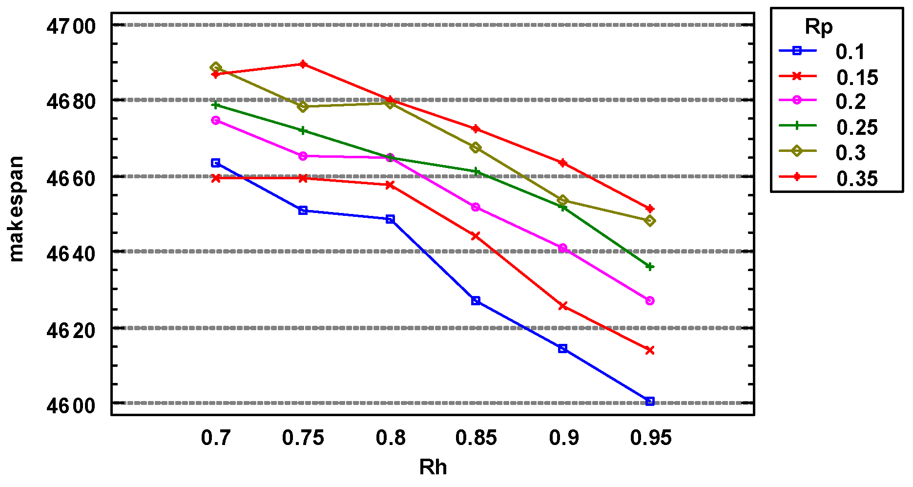
Figure 2.
Analysis of parameter rh.
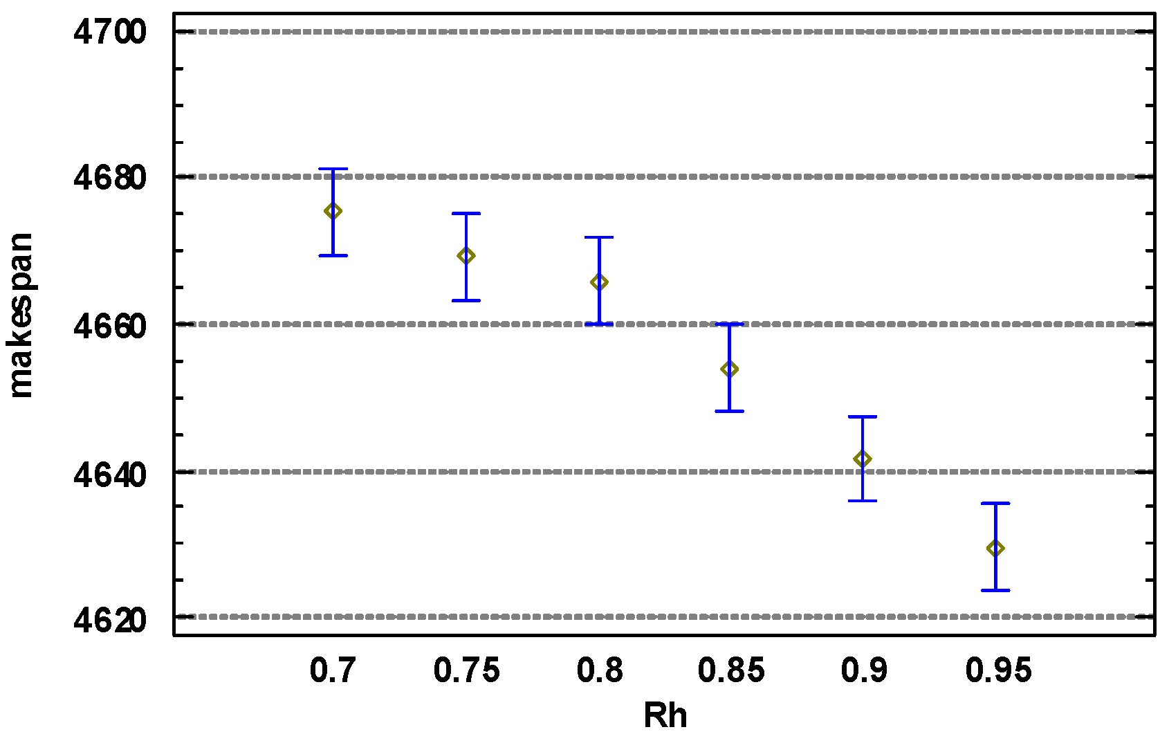
Figure 3.
Analysis of parameter rp.
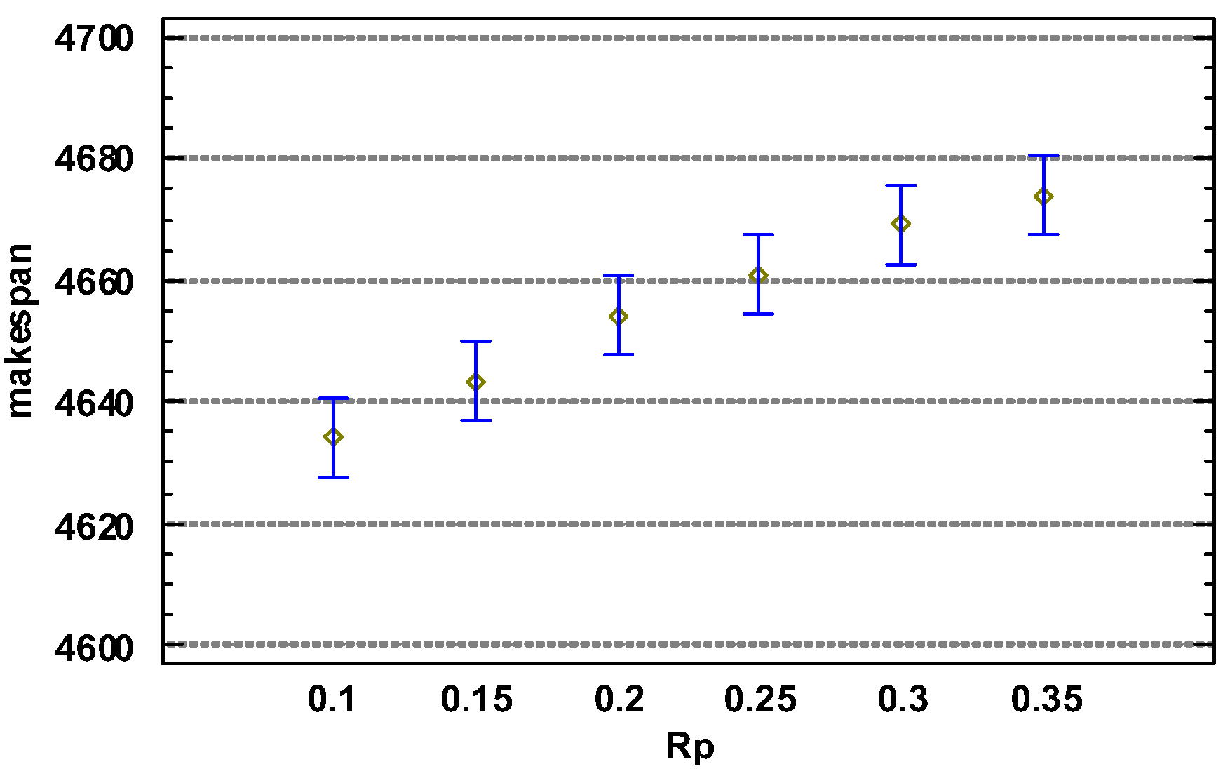
Figure 4.
Multivariate analysis of variance for job and algorithm.
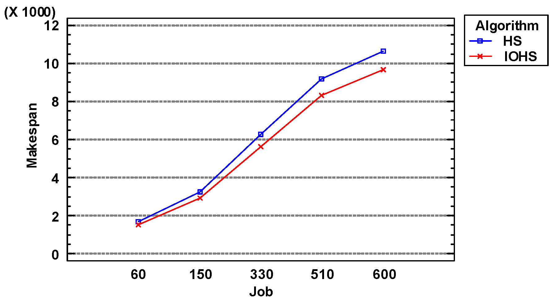
Figure 5.
Multivariate analysis of variance for factory and algorithm.
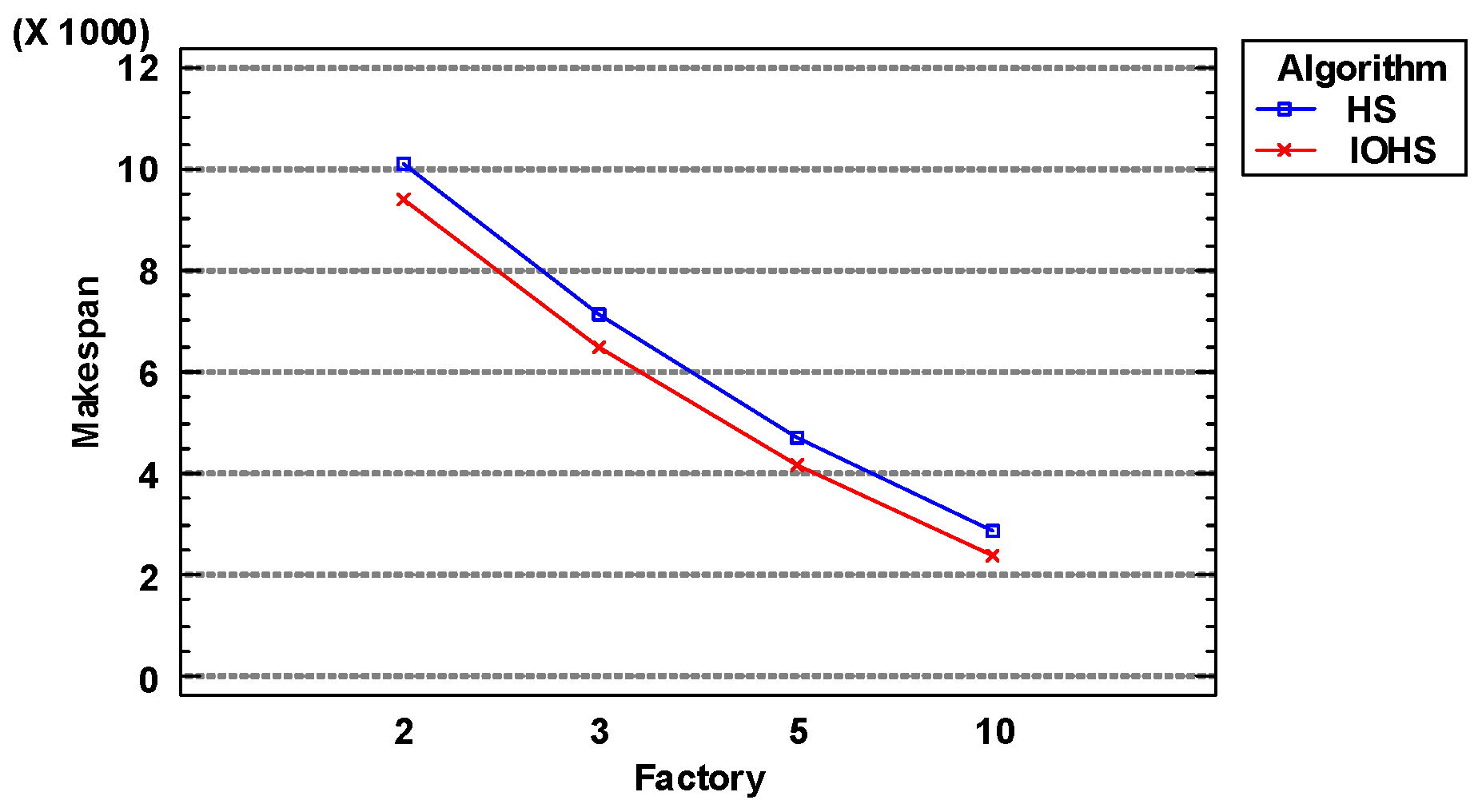
Figure 6.
Multivariate analysis of variance for machine and algorithm.
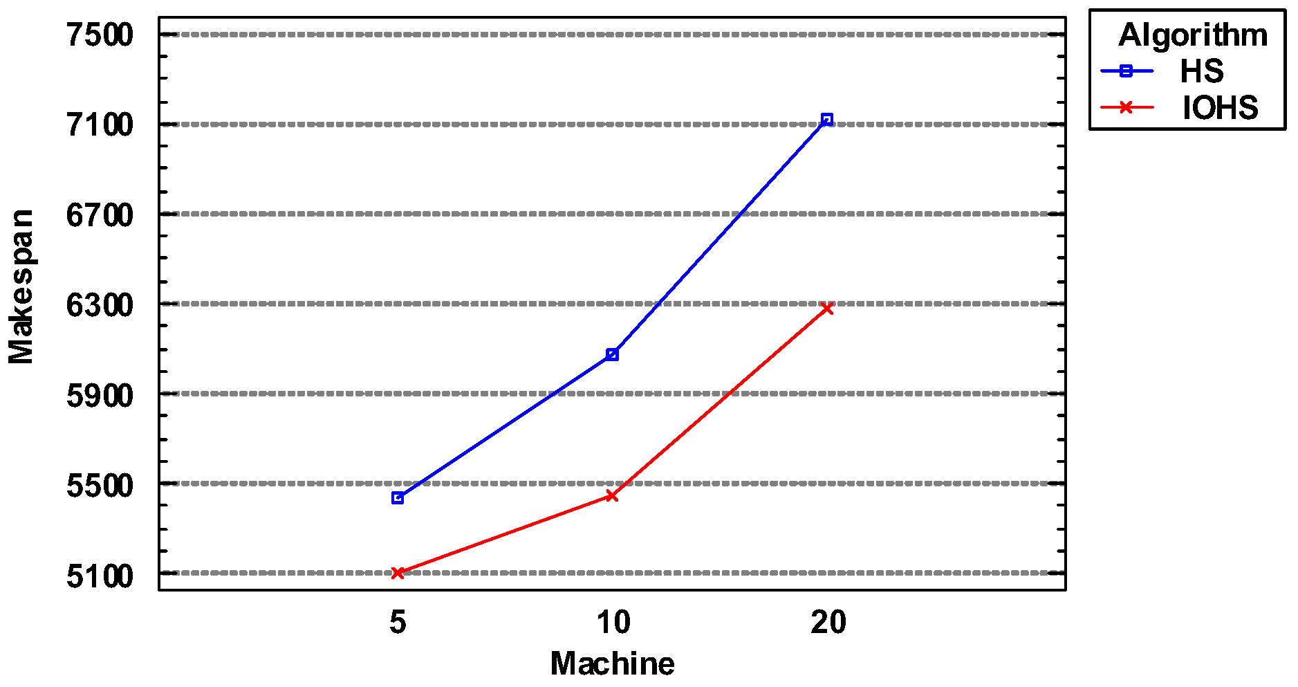
Figure 7.
The multi-factor ANOVA(Job and algorithm).
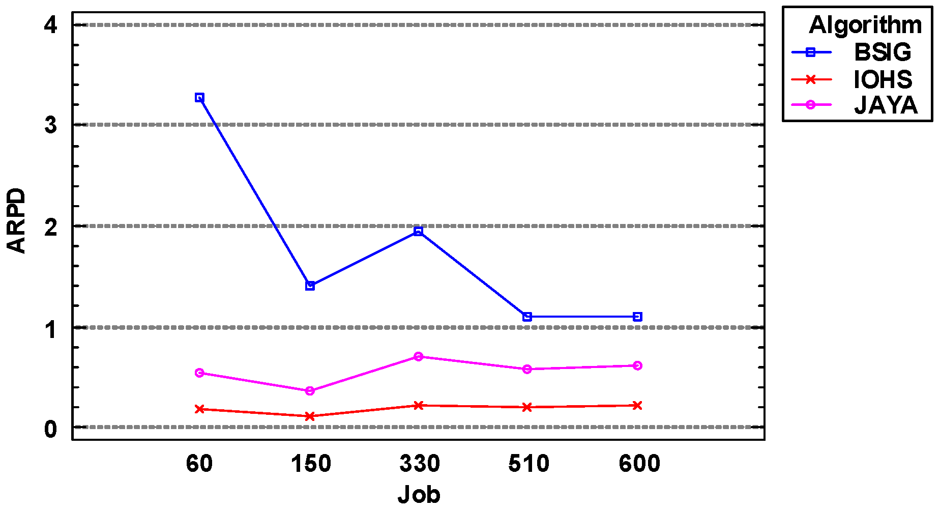
Figure 8.
The multi-factor ANOVA(Factory and algorithm).
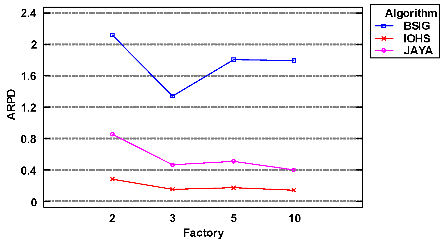
Figure 9.
The multi-factor ANOVA(Machine and algorithm).
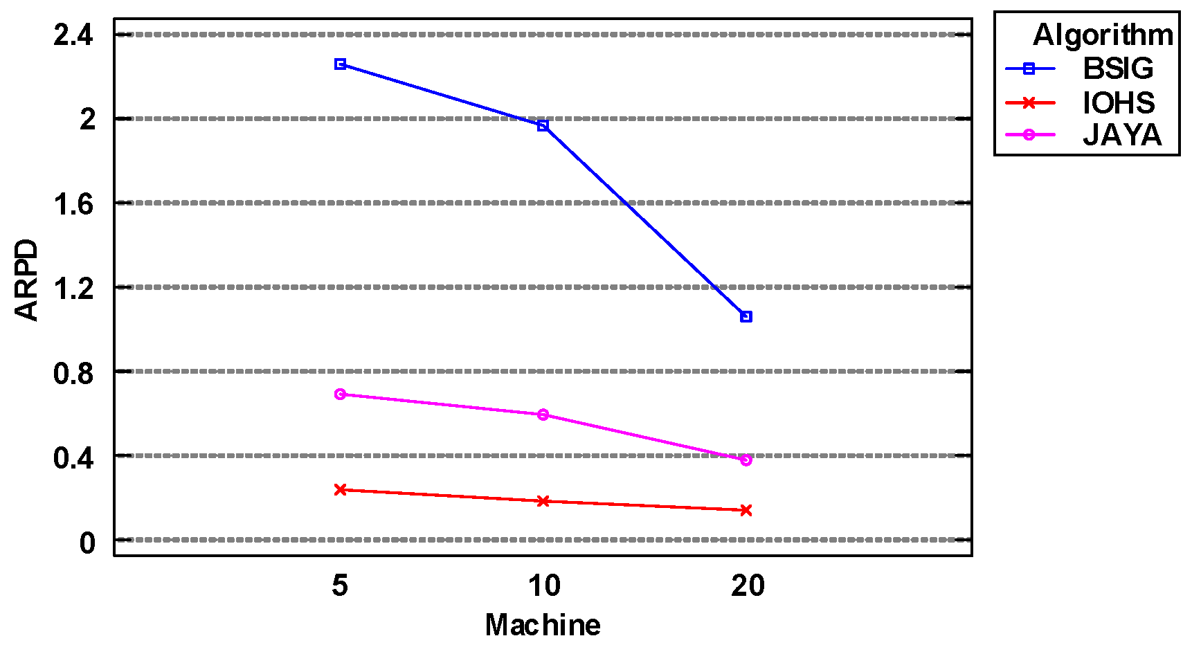

Table 1.
An example of HM.
| solution structure | job sequence | ||
| Processing Factory 1 | Processing Factory 2 | Processing Factory 3 | |
| {3,3,3} | {1,3,4} | {2,5,9} | {6,7,8} |
| {4,2,3} | {1,3,4,9} | {2,5} | {6,7,8} |
Table 2.
Comparison of parameter combinations.
| , | MSave | , | MSave | , | MSave |
| 0.7, 0.1 | 4663 | 0.8, 0.1 | 4648 | 0.9, 0.1 | 4614 |
| 0.7, 0.15 | 4659 | 0.8, 0.15 | 4658 | 0.9, 0.15 | 4626 |
| 0.7, 0.2 | 4675 | 0.8, 0.2 | 4665 | 0.9, 0.2 | 4641 |
| 0.7, 0.25 | 4679 | 0.8, 0.25 | 4665 | 0.9, 0.25 | 4652 |
| 0.7, 0.3 | 4689 | 0.8, 0.3 | 4679 | 0.9, 0.3 | 4654 |
| 0.7, 0.35 | 4687 | 0.8, 0.35 | 4680 | 0.9, 0.35 | 4663 |
| 0.75, 0.1 | 4651 | 0.85, 0.1 | 4627 | 0.95, 0.1 | 4601 |
| 0.75, 0.15 | 4659 | 0.85, 0.15 | 4644 | 0.95, 0.15 | 4614 |
| 0.75, 0.2 | 4666 | 0.85, 0.2 | 4652 | 0.95, 0.2 | 4627 |
| 0.75, 0.25 | 4672 | 0.85, 0.25 | 4661 | 0.95, 0.25 | 4636 |
| 0.75, 0.3 | 4678 | 0.85, 0.3 | 4667 | 0.95, 0.3 | 4648 |
| 0.75, 0.35 | 4689 | 0.85, 0.35 | 4673 | 0.95, 0.35 | 4651 |
Table 3.
Comparison of HS and IOHS.
| J,M,F | MSave | J,M,F | MSave | J,M,F | MSave | |||
| HS | IOHS | HS | IOHS | HS | IOHS | |||
| 60, 2, 5 | 1847 | 1774 | 150, 5, 20 | 3285 | 2858 | 510, 3, 10 | 10483 | 9442 |
| 60, 2, 10 | 2318 | 2119 | 150, 10, 5 | 1203 | 965 | 510, 3, 20 | 11782 | 10365 |
| 60, 2, 20 | 3102 | 2871 | 150, 10, 10 | 1618 | 1333 | 510, 5, 5 | 6049 | 5528 |
| 60, 3, 5 | 1349 | 1237 | 90, 10, 20 | 2333 | 2009 | 510, 5, 10 | 6748 | 5837 |
| 60, 3, 10 | 1751 | 1587 | 330, 2, 5 | 9159 | 8866 | 510, 5, 20 | 7913 | 6789 |
| 60, 3, 20 | 2485 | 2284 | 330, 2, 10 | 10007 | 9230 | 510, 10, 5 | 3351 | 2834 |
| 60, 5, 5 | 937 | 817 | 330, 2, 20 | 11374 | 10195 | 510, 10, 10 | 3893 | 3200 |
| 60, 5, 10 | 1308 | 1166 | 330, 3, 5 | 6314 | 5932 | 510, 10, 20 | 4846 | 4053 |
| 60, 5, 20 | 1977 | 1810 | 330, 3, 10 | 7078 | 6322 | 600, 2, 5 | 16347 | 15977 |
| 60, 10, 5 | 626 | 525 | 330, 3, 20 | 8237 | 7223 | 600, 2, 10 | 17485 | 16365 |
| 60, 10, 10 | 962 | 838 | 330, 5, 5 | 4020 | 3615 | 600, 2, 20 | 19138 | 17279 |
| 60, 10, 20 | 1593 | 1450 | 330, 5, 10 | 4651 | 3974 | 600, 3, 5 | 11205 | 10692 |
| 150, 2, 5 | 4373 | 4214 | 330, 5, 20 | 5667 | 4857 | 600, 3, 10 | 12137 | 11008 |
| 150, 2, 10 | 4907 | 4477 | 330, 10, 5 | 2280 | 1881 | 600, 3, 20 | 13560 | 11979 |
| 150, 2, 20 | 5923 | 5293 | 330, 10, 10 | 2787 | 2264 | 600, 5, 5 | 7060 | 6478 |
| 150, 3, 5 | 3037 | 2819 | 330, 10, 20 | 3634 | 3039 | 600, 5, 10 | 7806 | 6819 |
| 150, 3, 10 | 3571 | 3137 | 510, 2, 5 | 14136 | 13810 | 600, 5, 20 | 9002 | 7745 |
| 150, 3, 20 | 4502 | 3972 | 510, 2, 10 | 14994 | 13997 | 600, 10, 5 | 3863 | 3295 |
| 150, 5, 5 | 1998 | 1733 | 510, 2, 20 | 16599 | 14947 | 600, 10, 10 | 4464 | 3687 |
| 150, 5, 10 | 2465 | 2102 | 510, 3, 5 | 9528 | 9057 | 600, 10, 20 | 5437 | 4529 |
Table 4.
Comparison of algorithms.
| J,F,M | MSave | J,F,M | MSave | J,F,M | MSave | ||||||
| BSIG | Jaya | IOHS | BSIG | Jaya | IOHS | BSIG | Jaya | IOHS | |||
| 60,2,5 | 1828 | 1782 | 1774 | 150,5,20 | 3004 | 2887 | 2858 | 510,3,10 | 9719 | 9503 | 9442 |
| 60,2,10 | 2249 | 2144 | 2119 | 150,10,5 | 972 | 992 | 965 | 510,3,20 | 10761 | 10445 | 10365 |
| 60,2,20 | 3024 | 2897 | 2871 | 150,10,10 | 1342 | 1365 | 1333 | 510,5,5 | 5640 | 5556 | 5528 |
| 60,3,5 | 1248 | 1254 | 1237 | 90,10,20 | 2024 | 2044 | 2009 | 510,5,10 | 6085 | 5912 | 5837 |
| 60,3,10 | 1613 | 1618 | 1587 | 330,2,5 | 8941 | 8867 | 8866 | 510,5,20 | 7084 | 6853 | 6789 |
| 60,3,20 | 2318 | 2321 | 2284 | 330,2,10 | 9451 | 9244 | 9230 | 510,10,5 | 2940 | 2881 | 2834 |
| 60,5,5 | 828 | 841 | 817 | 330,2,20 | 10575 | 10217 | 10195 | 510,10,10 | 3354 | 3258 | 3200 |
| 60,5,10 | 1182 | 1193 | 1166 | 330,3,5 | 6036 | 5939 | 5932 | 510,10,20 | 4234 | 4094 | 4053 |
| 60,5,20 | 1833 | 1845 | 1810 | 330,3,10 | 6567 | 6363 | 6322 | 600,2,5 | 16042 | 15980 | 15977 |
| 60,10,5 | 534 | 544 | 525 | 330,3,20 | 7530 | 7277 | 7223 | 600,2,10 | 16647 | 16399 | 16365 |
| 60,10,10 | 855 | 867 | 838 | 330,5,5 | 3713 | 3641 | 3615 | 600,2,20 | 17773 | 17379 | 17279 |
| 60,10,20 | 1472 | 1484 | 1450 | 330,5,10 | 4181 | 4028 | 3974 | 600,3,5 | 10804 | 10707 | 10692 |
| 150,2,5 | 4270 | 4215 | 4214 | 330,5,20 | 5081 | 4894 | 4857 | 600,3,10 | 11299 | 11065 | 11008 |
| 150,2,10 | 4655 | 4482 | 4477 | 330,10,5 | 1973 | 1920 | 1881 | 600,3,20 | 12389 | 12062 | 11979 |
| 150,2,20 | 5544 | 5295 | 5293 | 330,10,10 | 2386 | 2308 | 2264 | 600,5,5 | 6601 | 6512 | 6478 |
| 150,3,5 | 2897 | 2828 | 2819 | 330,10,20 | 3180 | 3072 | 3039 | 600,5,10 | 7065 | 6894 | 6819 |
| 150,3,10 | 3325 | 3176 | 3137 | 510,2,5 | 13899 | 13811 | 13810 | 600,5,20 | 8065 | 7808 | 7745 |
| 150,3,20 | 4164 | 4008 | 3972 | 510,2,10 | 14225 | 14006 | 13997 | 600,10,5 | 3402 | 3343 | 3295 |
| 150,5,5 | 1823 | 1765 | 1733 | 510,2,20 | 15393 | 15016 | 14947 | 600,10,10 | 3871 | 3763 | 3687 |
| 150,5,10 | 2225 | 2141 | 2102 | 510,3,5 | 9160 | 9073 | 9057 | 600,10,20 | 4742 | 4580 | 4529 |
Table 5.
Comparison of algorithms based on ARPD.
| J,F,M | ARPD (%) | J,F,M | ARPD (%) | J,F,M | ARPD (%) | ||||||
| BSIG | Jaya | IOHS | BSIG | Jaya | IOHS | BSIG | Jaya | IOHS | |||
| 60,2,5 | 5.04 | 2.37 | 1.12 | 150,5,20 | 0.90 | 0.19 | 0.06 | 510,3,10 | 1.15 | 0.53 | 0.16 |
| 60,2,10 | 7.69 | 2.15 | 0.37 | 150,10,5 | 3.12 | 0.23 | 0.06 | 510,3,20 | 0.79 | 0.49 | 0.18 |
| 60,2,20 | 0.87 | 0.24 | 0.10 | 150,10,10 | 2.15 | 0.21 | 0.08 | 510,5,5 | 1.77 | 0.88 | 0.29 |
| 60,3,5 | 2.14 | 0.13 | 0.04 | 150,10,20 | 1.52 | 0.19 | 0.07 | 510,5,10 | 1.43 | 0.66 | 0.18 |
| 60,3,10 | 2.32 | 0.24 | 0.10 | 330,2,5 | 4.14 | 1.60 | 0.35 | 510,5,20 | 0.70 | 0.44 | 0.16 |
| 60,3,20 | 1.61 | 0.17 | 0.06 | 330,2,10 | 2.31 | 0.63 | 0.20 | 510,10,5 | 0.82 | 0.54 | 0.20 |
| 60,5,5 | 3.67 | 0.22 | 0.07 | 330,2,20 | 1.09 | 0.51 | 0.20 | 510,10,10 | 0.86 | 0.56 | 0.26 |
| 60,5,10 | 2.78 | 0.26 | 0.09 | 330,3,5 | 2.62 | 0.84 | 0.27 | 510,10,20 | 0.56 | 0.35 | 0.15 |
| 60,5,20 | 2.01 | 0.18 | 0.05 | 330,3,10 | 2.04 | 0.62 | 0.20 | 600,2,5 | 1.23 | 0.59 | 0.21 |
| 60,10,5 | 4.72 | 0.25 | 0.09 | 330,3,20 | 1.10 | 0.52 | 0.19 | 600,2,10 | 1.04 | 0.55 | 0.18 |
| 60,10,10 | 3.87 | 0.21 | 0.05 | 330,5,5 | 3.18 | 0.87 | 0.30 | 600,2,20 | 0.66 | 0.41 | 0.17 |
| 60,10,20 | 2.66 | 0.17 | 0.07 | 330,5,10 | 2.28 | 0.76 | 0.28 | 600,3,5 | 1.31 | 0.83 | 0.30 |
| 150,2,5 | 1.64 | 0.28 | 0.07 | 330,5,20 | 1.24 | 0.57 | 0.21 | 600,3,10 | 1.17 | 0.64 | 0.24 |
| 150,2,10 | 1.33 | 0.87 | 0.28 | 330,10,5 | 1.31 | 0.59 | 0.20 | 600,3,20 | 0.69 | 0.49 | 0.20 |
| 150,2,20 | 1.06 | 0.79 | 0.26 | 330,10,10 | 1.00 | 0.50 | 0.18 | 600,5,5 | 1.58 | 0.78 | 0.30 |
| 150,3,5 | 0.62 | 0.39 | 0.15 | 330,10,20 | 0.99 | 0.37 | 0.12 | 600,5,10 | 1.29 | 0.71 | 0.24 |
| 150,3,10 | 0.66 | 0.30 | 0.07 | 510,2,5 | 1.56 | 0.68 | 0.23 | 600,5,20 | 0.79 | 0.49 | 0.17 |
| 150,3,20 | 0.55 | 0.19 | 0.07 | 510,2,10 | 1.29 | 0.66 | 0.27 | 600,10,5 | 1.45 | 0.77 | 0.25 |
| 150,5,5 | 1.94 | 0.40 | 0.11 | 510,2,20 | 0.78 | 0.50 | 0.17 | 600,10,10 | 1.27 | 0.64 | 0.23 |
| 150,5,10 | 1.44 | 0.22 | 0.07 | 510,3,5 | 1.39 | 0.55 | 0.13 | 600,10,20 | 0.67 | 0.41 | 0.15 |
Disclaimer/Publisher’s Note: The statements, opinions and data contained in all publications are solely those of the individual author(s) and contributor(s) and not of MDPI and/or the editor(s). MDPI and/or the editor(s) disclaim responsibility for any injury to people or property resulting from any ideas, methods, instructions or products referred to in the content. |
© 2025 by the authors. Licensee MDPI, Basel, Switzerland. This article is an open access article distributed under the terms and conditions of the Creative Commons Attribution (CC BY) license (http://creativecommons.org/licenses/by/4.0/).
Copyright: This open access article is published under a Creative Commons CC BY 4.0 license, which permit the free download, distribution, and reuse, provided that the author and preprint are cited in any reuse.


