
Submitted:
01 July 2025
Posted:
02 July 2025
You are already at the latest version
Abstract
The purpose of the present paper is to present an efficient numerical model for the study of a nonlinear solid mechanics problem: the wrinkling in film/substrate systems, either planar or spherical. This numerical model will be based both on the Finite Element Method (FEM) and the Asymptotic Numerical Method (ANM). The mathematical and numerical aspects of ANM are given. ANM is a robust continuation method for solving nonlinear problems depending on a loading parameter. This technique has already been applied successfully to various fields in solid and fluid mechanics. We will present, with both theoretical and algorithm aspects, how ANM is used for solving nonlinear mechanical and nonlinear thermo-mechanical problems involving elastic behavior and geometrical nonlinearities. Then we propose the technical implementation of ANM for FEM in the framework of FreeFEM++. FEM software development platform, called FreeFEM++, because of its natural way to deal with variational formulations, is well adapted to implement ANM for instability problems in solid mechanics. In order to illustrate the great efficiency of FreeFEM++, we will show how to write elegant FreeFEM++ scripts to compute the different steps of ANM continuation for solid elastic structures considering simple geometries subjected to conservative loading. For validation purpose, we will show first the case of simple geometries, like a cantilever subjected to an applied force. The case of planar or spherical film/substrate systems will be studied in great details using the new developed numerical model. More precisely, we will show that this numerical model allows for the accurate prediction of equilibrium path in buckling analysis.
Keywords:
implicit function theorem
; partial differential equations
; asymptotic numerical method
; finite element method
; domain-specific language
; FreeFEM++
; film/substrate system
; wrinkling
1. Introduction
The wrinkle phenomena of thin membranes [1] or film-substrate systems [2] are very common in the recent literature. The numerical modeling of these instabilities may be highly complicated due to the existence of many equilibrium solutions and the poor stiffness of unloaded membranes. In such a situation, it is not easy to apply a continuation algorithm that may fails [1,3] or undergoes back-and-forth loops [4]. Such a difficulty may be avoided by using a pseudo-dynamic algorithm, e.g. [3,5,6]. In order to assess the limit of validity of continuation techniques in the quasi-static regime, we consider in this paper ANM with applications to film-substrate systems.
ANM is a continuation method based on Taylor series. It is associated with classical discretization techniques, generally the Finite Element Method (FEM). The coupling between a perturbation technique and FEM was first proposed by Thompson and Walker [7]. In [8,9,10], a continuation method was introduced together with an efficient procedure to build the Taylor series and the convergence acceleration using Padé approximants. Then ANM has been successfully applied to various engineering and scientific problems in solid and fluid mechanics [11,12,13,14,15,16,17]. It is rather different from classical incremental-iterative methods such as Riks strategy [18], because full solution paths are computed and not only pointwise solutions and because the a posteriori estimation of the radius of convergence ensures an optimal loading step size.
ANM has been implemented using various computer languages: FORTRAN 77, FORTRAN 90, MATLAB, C++. Many home-made implementations were established. For example, the open source software MANLAB [19] is widely used in the field of nonlinear vibrations. Lejeune et al. [20] described a full object-oriented implementation within C++. Nonetheless, the home-made software is difficult to maintain and often provides a framework that is not enough user-friendly. Application in fluid mechanics within the open source finite element platform ELMER has been done and results were presented in [21].
FreeFEM++ [22] is a very efficient environment to implement variational formulations. As we will show in this paper, FreeFEM++ uses a high level language that allows to derive very easily variational formulation and to implement the ANM algorithm. The main idea is to develop a general, and easy to use, environment to implement the ANM algorithm for solving solid mechanical problems. FreeFEM++ also offers MPI parallel solvers and multigrid or domain decomposition tools that enables to reduce the CPU time and gives the opportunity to take into account large number of degrees of freedom. In this paper, the implementation of ANM in the FreeFEM++ code is discussed. Let us mention a publication regarding the analysis of infinite periodic surface acoustic waves transducers using FreeFEM++ [23] and a recent publication about fluid-structure interaction problems solved using FreeFEM++ [24].
The second section will present the main mathematical aspects of ANM. The third section the application of ANM in the case of nonlinear solid elastic problems. And the fourth section is dedicated to thermo-elastic nonlinear problems. The fifth section we will show what makes FreeFEM++ an efficient tool to implement ANM for various nonlinear mechanical problems, and will describe the implementation of the ANM algorithm in FreeFEM++. The sixth section presents the simulation results, using the FreeFEM++ implementation of ANM, of the nonlinear mechanical behavior of a clamped cantilever and subjected to a vertical surface force at its right surface, of a planar film/substrate system under uni-axial loading [25,26], and of a spherical film/substrate system subjected to a thermo-mechanical shrinkage of its core [3].
2. Theoretical Aspects of ANM
Let us recall the mathematical aspects of the Asymptotic Numerical Method (ANM) [27][28]. Let us begin with the resolution of the equation (1) in the case of a finite n-dimensional vectorial space:
with, , , and
Generally, the problem (1) is formulated for belonging to a Banach space, but here we will considered problems coming from engineering, and physics, formulated in a discretized space using a numerical method like the Finite Element Method or using only a finite number of degrees of freedom.
Let us now assume that the function is a class function (with ) from where H is an open set of and I is an open segment of and that for , the partial differential is a bi-continuous isomorphism. The implicit function theorem [29] states that the equation (1) has a unique solution branch from a neighborhood of in I to H, which is also a class function.
Furthermore, if we assume that is an analytic function, the function is also analytic and it is possible to expand both and into serial using the parameter a called path parameter within a given radius of convergence [28][30][31]:
Let us explain the algebraic properties of the ANM. If we consider a given function , as detailed in [28], the i-th derivative of is a function of all the derivative of up to order i. Furthermore, we have the general expression:
Let us notice that there is a linear relationship between and with the same Jacobian matrix for each order, and, that is a multilinear function of previous orders. As a consequence, the expression (3) for allows to obtain the matrix since , and, at order , by assuming , the expression is given by .
3. ANM for Elastic Nonlinear Problems
3.1. Theory
Let us explain how the Asymptotic Numerical Method (ANM) can be applied in the case of quasi static geometrically nonlinear elastic problems [8,9,10].
The considered elasticity model, known as the Saint Venant-Kirchhoff law, is a linear relation between the second Piola-Kirchhoff stress tensor and the Green-Lagrange strain tensor defined by the following:
and its variation is given by:
The formulation of the full boundary value problem is quite classical and combines the elastic constitutive law with the virtual work equation
where is the elastic stiffness tensor, is a scalar load parameter and represents the given force on the part of the boundary .
Each step of ANM relies on a Taylor series according to a well chosen path parameter a:
Several efficient choices of the path parameter are available [32]. The most popular one is a linearized arc-length parameter that permits us to easily bypass all the extrema of the response curves. It is given by [27]:
where (resp. ) are normalized displacement vector (resp. loading parameter). Here, by default, we will use (resp. ).
When the Taylor series (7) are substituted into Eqs.(6-8). Identifying mathematical expressions related to a given order p in a results in a linear system. Here, the boundary value problem in Eq.(6) has a simple structure, the equations involving only linear and quadratic terms with respect to the unknown fields and this system can be deduced from the usual Leibniz rule to compute high-order derivatives, or equivalently, the Taylor coefficients of a product: . First of all, let us identify the coefficients at order 1 in a, which yield the classical tangent variational problem, as in Newton-Raphson’s method:
where the bilinear form is the classical tangent stiffness operator given by:
And the linear form related to the virtual work of external forces is given by:
The definition in Eq. (8) of the path parameter gives an additional equation:
At the order in a, we get also a variational formulation involving the same bilinear form :
The last term is a linear depends on the variables at orders . It is given by:
while the stress on order p is:
The last is the arc-length condition in Eq. (8) yields the load parameter as a function of the displacement :
Usually, the Taylor expansion order is chosen between 15 and 50 to take advantage of the exponential convergence of power series. Of course, the path parameter a is required to be inferior to the convergence radius of the series 7. In fact, We will ask the truncated Taylor series to verify a given accuracy: the normalized norm of the difference between the two last order in the Taylor series is asked to be inferior to a given parameter which results for the following inequality to be verified: . This will leads to the expression of the path parameter called validity parameter:
In this way, the Taylor expansion (7) gives a part of the solution path in the interval . The continuation procedure may be very simple by chaining several series, the end point of this path being the starting point of the next step. It is also possible to improve the accuracy of the end point by using a corrective step via Newton method or the high-order method [33] or by applying a convergence acceleration technique [34]. The Newton-Riks correction method can be easily implemented in the FreeFem++ environment.
3.2. Numerical Algorithm
Let us now describe how to derive a numerical model from the variational formulation established in the previous chapter using the Finite Element Method (FEM). The finite element implementation of the ANM is described in the section 7 of [27].
Let us now describe the main steps for the implementation of the resolution of a mechanical problem with geometrical nonlinearities using the ANM algorithm in the FreeFEM++ language. The ANM algorithm is detailed below (Algorithm 1):
| Algorithm 1 Algorithm ANM |
|
The FEM stiffness matrix is the implementation of the bilinear form (10), the FEM right-hand side vector is the implementation of the linear form (11), and the FEM right-hand side vector is the implementation of the linear form (14). The main details of the implementation in FreeFEM++ will be given in the Section 5. The algorithm A3 of the Newton-Riks correction is given in the Appendix (B) as well as the algorithm A2 of Newton-Raphson predictions which will be used later for comparison purpose.
4. ANM for Thermo-Elastic Nonlinear Problems
4.1. Theory
In this section, we show that it is possible to take into account an isotropic thermal expansion (or shrinkage) of an elastic domain with the ANM. As in the previous section, we assume that the domain is a Saint Venant-Kirchhoff material and we will consider nonlinear geometric elasticity, as in previous section. This domain will be subjected to isotropic thermal expansion (or shrinkage), driven by the scalar parameter .
We will assume that the thermomechanical effects result in an additional contribution to the Green-Lagrange strain tensor (4)), and its expression is (where is the identity matrix). Notice that the expression of (5) is not changed.
Incorporating thermal effects, the virtual work equation (6) results in the following:
means a thermo-elastic shrinkage.
Let us present how to incorporate the thermo-elastic formulation within the ANM algorithm. We can easily derive the expression of at the order :
The additional equation for the path parameter is the same than Eq. 12.
The bilinear form is the classical tangent stiffness operator already given in (10), and the linear form that accounts for the thermomechanical shrinkage is given by:
Notice that the integrand on the right member of (21) is the trace of the second-rank tensor .
At order , we obtain a variational form involving the same bilinear form, and the linear form accounting for the nonlinear second member has the same expression as in Section 3 (see equation (14)).
The additional equation for the path parameter is the same than Eq. 16.
4.2. Numerical Algorithm
The ANM numerical algorithm for the thermo-elastic nonlinear problem is very close to the algorithm (1) presented in Section 3.2. The only difference relies in the FEM right-hand side vector , which is now the implementation of the linear form (21).
5. Some Aspects of the FreeFEM++ Implementation
FreeFEM++ is based on an efficient Domain-Specific Language (DSL) which allows partial differential equations and more generally nonlinear multiphysics systems in 2D, 3D, and on surface to be solved. The FreeFEM++ language is typed, polymorphic and reentrant with macro generation. The kernel of FreeFEM++ is written in C++.
Let us now resume the main characteristics of FreeFEM++:
- FreeFEM++ has a high level user friendly typed input language with an algebra of analytic and finite element functions.
- The finite element problems are described by their variational formulations, and are easily implemented. It is possible to have access to the internal vectors and matrices if needed.
- Many kinds of problems can be solved: multi-variables, multi-equations, one, two or three dimensional static or time dependent, linear or nonlinear coupled systems.
- An automatic mesh generator is available, based on the Delaunay-Voronoï algorithm.
- A large variety of triangular finite elements: linear and quadratic Lagrangian finite elements and more, discontinuous P1, and Raviart-Thomas elements.
- A large variety of linear direct and iterative solvers (LU, Cholesky, Crout, CG, GMRES, UMFPACK, MUMPS, SuperLU, ...), eigenvalue and eigenvector solvers (ARPACK) are available.
Most of these characteristics are of great interest for simulating nonlinear mechanical problems using the ANM continuation algorithm. As we will see in more detail in the following, the mesh generator is very easy to use for simple geometries, the macro generation enables us an easy implementation of the differential operators useful in nonlinear solid mechanics, and the variational formulation oriented commands in FreeFEM++ allows us to implement very efficiently the weak form of nonlinear solid mechanical differential equations, discretized using the Finite Element Method.
Let us present the main steps of the Finite Element Method discretization by getting closer to the FreeFEM++ implementation. In order to set these ideas down, let us begin with the Laplacian problem, a basic problem for applied mathematics.
We would like to find u a real function defined on a domain of such that:
with . The boundary condition on (resp. on ) is called Dirichlet (resp. Neumann) boundary conditions.
Let us define the functional space by:
Using the Green’s formula that generalizes the integration by part, an equivalent weak form (or variational form) of the previous problem (23) is obtained: Find such that:
The Finite Element Method starts with the partitioning of the initial domain into subdomains called elements. It results in the spatial discretization of the domain (mesh). In FreeFEM++ the 2D (resp. 3D) mesh, is partitioned into triangles (resp. tetrahedra).
FEM approximates all functions w as:
where N is the number of nodes of the mesh, depending on the FEM interpolation, detailed below. The restriction of the basis functions to each tetrahedron is called shape function.
The finite element space is defined by:
The list of finite elements available in the FreeFEM++ environment is wide: (piecewise constant discontinuous finite element), (piecewise linear continuous finite element), (piecewise linear discontinuous finite element), (piecewise continuous finite element), ...
First, let us focus on the elementary Laplacian problem (23). We will assume that the 3D mesh has already been generated and saved in the file "Th3D.msh". Let us load the mesh and build the finite element interpolation space on this mesh. This is done in FreeFEM++ with the two command lines:
- msh3 Th("Th3D.msh");
- fespace Vh(Th,P1);
Then, the differential operator gradient will be defined with the following commands macro:
- macro Grad(u) [dx(u), dy(u), dz(u)] //
Let us define u the solution function, v the test function, belonging to the finite element space , and implement the equivalent variational formulation of the Laplacian problem:
- Vh u,v;
- problem Poisson(u,v) =
- int3d(Th)(Grad(u)’*Grad(v))-int3d(Th)(f*v)
- -int2d(Th,LN)(g*v)
- +on(LD,u=0);
The first (resp. second) operator int3d is used for the bilinear part (resp. linear part) of the variational formulation (25). The operator int2d allows to take into account the Neumann boundary conditions (LN is the label of the mesh concerned with the Neumann boundary conditions), and the operator on(.) is used to describe the Dirichlet boundary conditions (here LD is the label of the mesh concerned with the Dirichlet boundary conditions).
The numerical solution of the problem (25) is obtained using the following command:
- Poisson;
It is also possible to plot the solution field u using the command:
- plot(u,wait=1);
It is easy to generalize the FreeFEM++ implementation of the Laplacian problem to the resolution of nonlinear mechanical problem using ANM. FreeFEM++ enables to generate directly the sparse Finite Element matrices, and the right-hand sides, and this is usefull regarding the implementation of ANM algorithm.
Let us now describe the main steps for the implementation of the resolution of a mechanical problem with geometrical nonlinearities using the ANM algorithm in the FreeFEM++ language. We will assume that the material is elastic with a Saint Venant-Kirchhoff constitutive law,
The FEM stiffness matrix is the implementation of the bilinear form (10), the FEM right-hand side vector is the implementation of the linear form (11), and the FEM right-hand side vector is the implementation of the linear form (14).
Differential operators, needed to define Green-Lagrange tensor and its variation are easily implemented in the FreeFEM++ language using a command macro. It represents one of the strength of FreeFEM++ for variational formulation implementation. For this purpose, let us present the main macro commands:
- macro GammaL(u,v,w) [dx(u),dy(v),dz(w),(dy(u)+dx(v)),
- (dz(u)+dx(w)),(dz(v)+dy(w))] //
- macro GammaNL(u1,v1,w1,u2,v2,w2)
- [(dx(u1)*dx(u2)+dx(v1)*dx(v2)+dx(w1)*dx(w2))*0.5,
- (dy(u1)*dy(u2)+dy(v1)*dy(v2)+dy(w1)*dy(w2))*0.5,
- (dz(u1)*dz(u2)+dz(v1)*dz(v2)+dz(w1)*dz(w2))*0.5,
- (dy(u1)*dx(u2)+dx(u1)*dy(u2)+dy(v1)*dx(v2)
- +dx(v1)*dy(v2)+dy(w1)*dx(w2)+dx(w1)*dy(w2))*0.5,
- (dz(u1)*dx(u2)+dx(u1)*dz(u2)+dz(v1)*dx(v2)
- +dx(v1)*dz(v2)+dz(w1)*dx(w2)+dx(w1)*dz(w2))*0.5,
- (dz(u1)*dy(u2)+dy(u1)*dz(u2)+dz(v1)*dy(v2)
- +dy(v1)*dz(v2)+dz(w1)*dy(w2)+dy(w1)*dz(w2))*0.5] //
- macro Gamma(u,v,w) (GammaL(u,v,w)+GammaNL(u,v,w,u,v,w)) //
- macro dGammaNL(u,v,w,uu,vv,ww) (2.0*GammaNL(u,v,w,uu,vv,ww)) //
- macro dGamma(u,v,w,uu,vv,ww) (GammaL(uu,vv,ww)+dGammaNL(u,v,w,uu,vv,ww)) //
Here, the classical Voigt notation has been used for the Green-Lagrange tensor.
GammaL(u,v,w) represents the linear part of the Green Lagrange tensor, and GammaNL(u1,v1,w1,u2,v2,w2)) ) its nonlinear part (4). The tensor dGammaNL(u,v,w,uu,vv,ww) is the variation of the non linear part of the Green Lagrange tensor (5).
Then, the elasticity matrix is easily implemented:
- real E = 1.e5; nu = 0.;
- real lambda = E*nu/(1.0+nu)/(1.0-2.0*nu); mu = E/2.0/(1.0+nu);
- func D = [
- [ (lambda+2.0*mu), lambda, lambda,0.0,0.0,0.0 ],
- [ lambda,(lambda+2.0*mu), lambda,0.0,0.0,0.0 ],
- [ lambda, lambda,(lambda+2.0*mu),0.0,0.0,0.0 ],
- [ 0.0,0.0,0.0,mu,0.0,0.0 ],
- [ 0.0,0.0,0.0,0.0,mu,0.0 ],
- [ 0.0,0.0,0.0,0.0,0.0,mu ]
- ];
E, nu are Young’s modulus and Poisson ratio, lambda, mu are Lamé’s coefficients and D is the elasticity matrix.
Let us now describe how to implement in the language FreeFEM++ the variational formulation which will lead to the computation of both stiffness matrix, and right-hand side vector.
P2 Lagrange FEM interpolation is assumed and defined on the mesh Th3D via the fespace command:
- fespace Vh(Th3D,[P2,P2,P2]);
Let us declare the displacement fields for each ANM order:
- Vh[int] [u,v,w](Norder+1);
Here, we will not use the previous command problem but the key command varf, which facilitates the computation of the tangent matrix and the linear right-hand side, while taking into account the Dirichlet boundary conditions (using the keyword on).
- varf PbTg ([u1,v1,w1],[uu,vv,ww]) =
- int3d(Th3D) ( (dGamma(u[0],v[0],w[0],uu,vv,ww))’*
- (D*(GammaL(u1,v1,w1)+2*GammaNL(u[0],v[0],w[0],u1,v1,w1)))
- +(dGammaNL(u1,v1,w1,uu,vv,ww))’*(D*(GammaL(u[0],v[0],w[0])
- +GammaNL(u[0],v[0],w[0],u[0],v[0],w[0]))) )
- +on(lencasmid,u1=0.,v1=0.,w1=0.);
- varf PbF ([u1,v1,w1],[uu,vv,ww]) = int2d(Th3D,lrigthmid) (Pa*ww)
- +on(lencasmid,u1=0.,v1=0.,w1=0.);
lrigthmid (resp. lencasmid) is the label of the mesh concerned with the vertical pressure (resp. Dirichlet boundary conditions).
The first varf PbTg is used to assemble the tangent matrix:
- matrix Kt = PbTg(Vh,Vh,solver=sparsesolver);
The second varf PbF is used to assemble the nodal vector of the linear right-hand side:
- Vh [Fu,Fv,Fw];
- Fu[] = PbF(0,Vh);
Let us now mention the important points appearing in the loop on the ANM orders for one ANM step.
First of all, the finite element displacement field is computed using a linear system resolution (we used the MUMPS direct solver, which has proven is efficiency).
- Vh [u1hat,v1hat,w1hat];
- u1hat[] = Kt^-1*Fu[];
It is now necessary to assemble the nonlinear right-hand side vector . Like it is done in the ANM algorithm (1), we define intermediate tensors (written in a vectorial form) and defined at the Gauss points:
- fespace QFh6(ThL3D,
- [FEQF53d,FEQF53d,FEQF53d,FEQF53d,FEQF53d,FEQF53d]);
- QFh6[int] [Sxx,Syy,Szz,deuxSxy,deuxSxz,deuxSyz](Norder+1);
- QFh6[Snlxx,Snlyy,Snlzz,deuxSnlxy,deuxSnlxz,deuxSnlyz](Norder+1);
The first step is to compute :
- [Sxx[1],Syy[1],Szz[1],deuxSxy[1],deuxSxz[1],deuxSyz[1]] =
- DL*(GammaL(u[1],v[1],w[1])+2*GammaNL(u[0],v[0],w[0],u[1],v[1],w[1]));
Then, we obtain :
- [Snlxx,Snlyy,Snlzz,deuxSnlxy,deuxSnlxz,deuxSnlyz] =
- DL*(GammaNL(u[1],v[1],w[1],u[1],v[1],w[1]));
It is now possible to assemble the nonlinear second member :
- varf PbFnl2 ([u1,v1,w1],[uuu,vvv,www]) = - int3d(Th3D) (
- (dGammaNL(u[1],v[1],w[1],uuu,vvv,www))’*
- ([Sxx[1],Syy[1],Szz[1],deuxSxy[1],deuxSxz[1],deuxSyz[1]])
- + (dGamma(u[0],v[0],w[0],uuu,vvv,www))’*
- ([Snlxx,Snlyy,Snlzz,deuxSnlxy,deuxSnlxz,deuxSnlyz]) )
- + on(lencasmid,u1=0.,v1=0.,w1=0.);
- Fnlu[]=PbFnl2(0,Vh);
Let us now enter the loop with respect to the order . All the FreeFEM++ implementation details are given in .
Let us now compute the norm of and to determine (17):
- real Norm1 = sqrt(int3d(Th3D) (u[1]’*u[1]+v[1]’*v[1]+w[1]’*w[1]));
- real NormNo = sqrt(int3d(Th3D) (u[Norder]’*u[Norder]+
- v[Norder]’*v[Norder]+
- w[Norder]’*w[Norder]));
- amax = (delta*Norm1/NormNo)^(1.0/(Norder-1.0));
The final task consists in evaluating the Taylor series of the displacement nodal vector, computing the residual error, and actualizing both and .
Let us mention that the FreeFEM++ scripts for the FEM simulation of non linear solid mechanics using ANM will be available soon in the FreeFEM++ web site (https://freefem.org/).
6. Numerical Results
In order to validate the FreeFEM++ program, the first section will focus on a simulation example based on a simple geometry. This is a clamped beam subjected to a vertical conservative surface traction. This problem has already been studied by Zahrouni [37] in the case of shell finite elements and a concentrated force. For validation purpose, we will add some simulation results obtained with the commercial software Abaqus. In the following section, we will briefly show that the FreeFEM++ simulation tool is able to simulate more complex structures like film/substrate systems under axial compression.
6.1. Clamped Beam Subjected to a Conservative Vertical Surface Traction
Consider a clamped beam subjected to a conservative load at its free end. The length of the beam is 10 mm, its width is 1 mm, and the thickness is 1 mm. The left face of the beam is clamped, and a conservative vertical traction is applied to the left face (see Figure 1).
The beam has been meshed using tetraedral P2 Lagrangian finite elements (see Figure 2).
The beam is supposed to be an homogeneous isotropic elastic material with Young’s modulus of , and 0 Poisson’s ratio. A FreeFEM++ script has been developed in order to simulate the non linear elastic behavior of the clamped beam. For building the finite element mesh of the beam, we choose 40 elements for its length, and 4 elements for its width and height. The ANM order is 15 and the ANM branch length is determined by . The amplitude of the surface traction is . Let us recall that the loading parameter appears in the weak form related to the applied force (right term of the second equation of (6)). Figure 3 shows the plot of the load parameter versus the vertical displacement of the center of the right face. We can see that FreeFEM++ and Abaqus computations are in a very good agreement. Large deflection up to have been obtained with only 7 ANM steps. At the end of each step, the normalized residual error is close to . Figure 3 shows the plot of the FreeFEM++ computations for the ANM orders 15, and 30. We can notice that, for the ANM order 30, the step length is greater than for the ANM order 15. Only 4 steps are needed for the whole curve when the ANM order is equal to 30.
When we choose the step length increases but the residual error increases roughly to .
6.2. Film-Substrate Systems Under Uniaxial Compression
We are now going to consider a more complex nonlinear mechanical problem: the film-substrate system. Surface morphological instabilities of a soft material with a stiff thin surface layer have been extensively studied over the past years.
When depositing a stiff thin film on a polymeric soft substrate, the developed residual compressive stresses in the film during the cooling process due to the large mismatch of thermal expansion coefficient between the film and the substrate, are relieved by buckling with wrinkling patterns, which was pioneered by Bowden et al. [38] in 1998. Let us notice that wrinkles of a thin stiff film deposited on a soft substrate can be widely used in industry for lots of applications, like the micro/nano fabrication of flexible electronic devices with controlled morphological patterns [39] [40], to the mechanical property measurement of material characteristic [41].
The film-substrate system being studied consists of a stiff film deposited on a soft rectangle parallelepiped substrate (Figure 4).
Film substrate systems has already been studied with the help of ANM using a coupling between shell finite element (Büchter-Ramm [42]) and hexahedron finite elements by Fan Xu et al. ([25,26]). In this section we will present a numerical model with ANM using only tetrahedron finite element (because of the FreeFEM++ implementation).
As in Fan Xu’s research, we will assume geometrical nonlinear elasticity for the stiff film, and linear elasticity for the soft substrate. The planes , , are symmetry planes of the modelled film-substrate system (only one fourth of the structure will be modelled). Moreover, on the interfaces , and, the vertical displacement is supposed zero. The length, width, and height of the substrate are respectively , , and, . The thickness of the film is .
The substrate and the film are supposed to be homogeneous isotropic and elastic materials. Young’s modulus of the substrate (resp. film), is (resp. ), and Poisson ratio of the substrate (resp. film) is (resp. ). Let us notice that the Young’s modulus of the film is much larger than that of the substrate (), which will allow to assume linear elasticity for the substrate domain while nonlinear geometrical elasticity will be assumed for the film domain [43]. The number of elements for both length and width of the film/substrate system is 100. We consider one element in the film thickness, and 5 elements in the substrate thickness. P2 Lagrange finite element interpolation is assumed. The mesh consists in 360000 tetraedra, and 1575639 degrees of freedom. We choose an ANM strategy with quite small steps (), and the ANM order is 15. One ANM step requires almost 40 minutes of CPU time when the FreeFEM++ program is parallized on 6 MPI processors while using the multifrontal MUMPS solver.
According to recent works [34] regarding acceleration convergence improvement of the ANM algorithm, MMPE extrapolation, adaptatives steps, and Newton Riks correction have been used. Let us give some details about these improvements. First, the total number of Newton’s corrections according to the parameter is presented in Table 1. We can see that both acceleration convergence and step adaptation are very efficient to reduce Newton Riks’s corrections.
The residual before and after the application of the acceleration MMPE are presented in (Table 2). Seven starting points with are considered. Step 34 has been chosen, with the full algorithm and . We can notice again the great efficiency of the MMPE convergence acceleration to improve the normalized residual error.
The bifurcation diagram is shown in Figure 5 which represents the vertical displacement of the center of the film-substrate system as a function of the load parameter . The accumulation of small steps in the diagram shows the presence of a bifurcation. Figure shows the comparison between the bifurcation diagram obtained with ANM (full algorithm) and a classical Newton-Raphson continuation algorithm with Newton-Riks correction.
Many bifurcations can be seen on the diagram of Figure (Figure 5). At the first bifurcation for , uniformly distributed one-dimensional wrinkles appears. Next the curve goes back for and five limit points are obtained that corresponds to the increase of a single wrinkle near the boundary and to a change of the number of wrinkles [34]. Small steps accumulate close to the limit points, which indicates that these singularities are in fact perturbed bifurcation points [44].
Figure 5.
Bifurcation diagram: vertical displacement of the center of the film-substrate system (top surface) with .
Figure 5.
Bifurcation diagram: vertical displacement of the center of the film-substrate system (top surface) with .
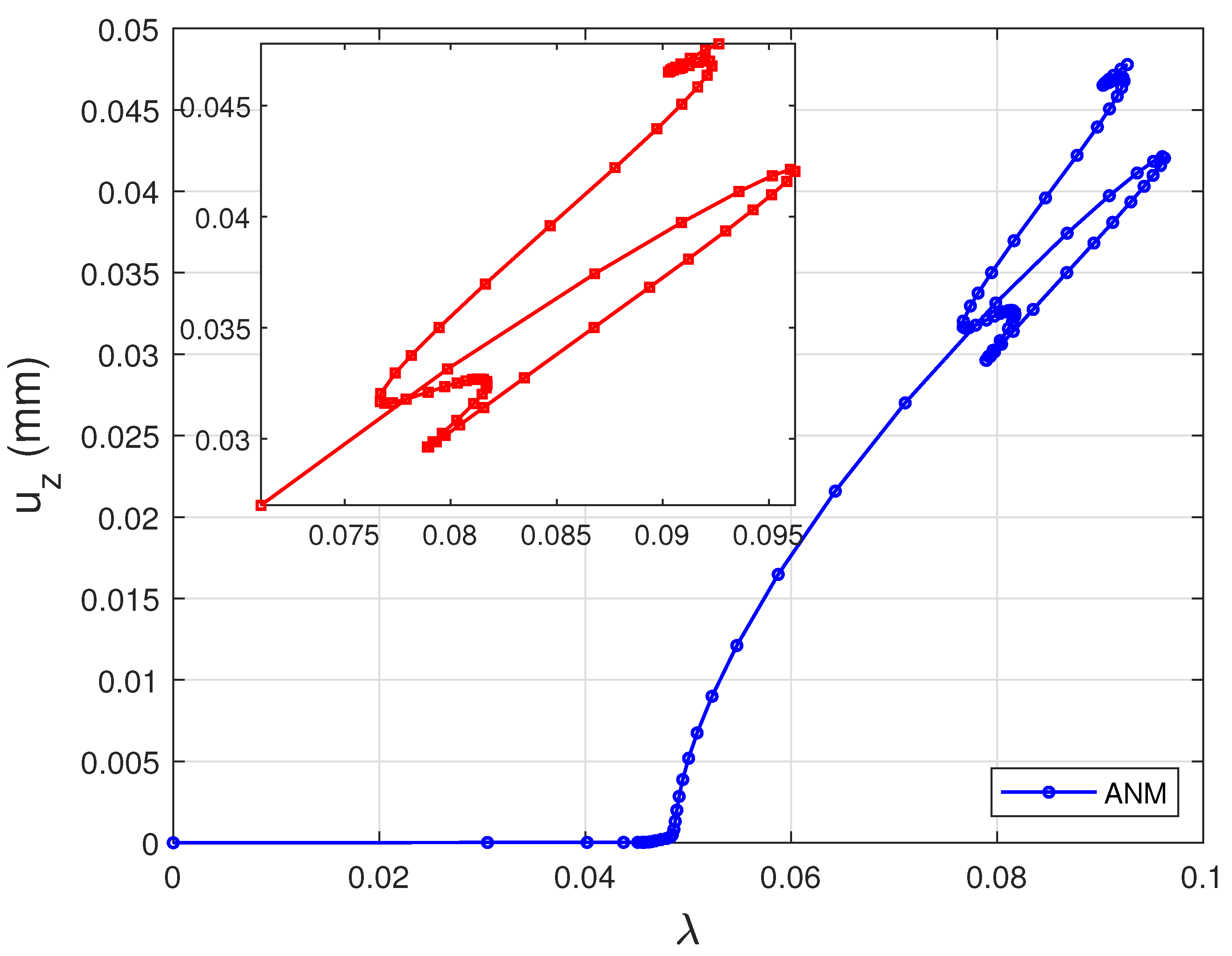
Figure 6.
Bifurcation diagram: vertical displacement of the center of the film-substrate system (top surface) with : comparison ANM full algorithm and Newton-Raphson continuation algorithm wit Newton-Riks like corrections.
Figure 6.
Bifurcation diagram: vertical displacement of the center of the film-substrate system (top surface) with : comparison ANM full algorithm and Newton-Raphson continuation algorithm wit Newton-Riks like corrections.
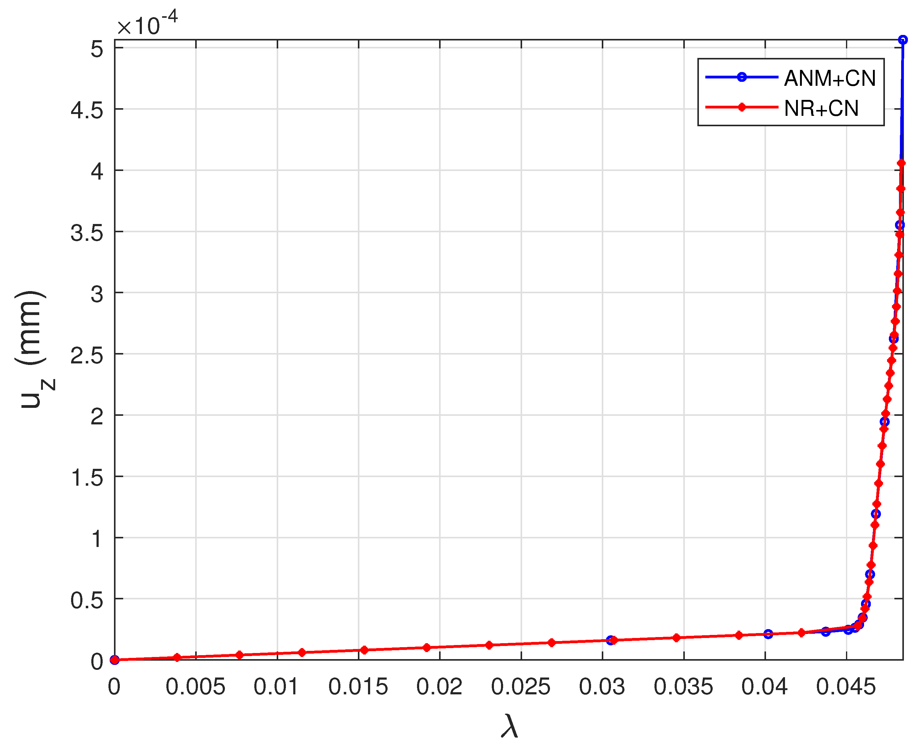
Figure 7.
Deformed of the film top surface just before the first bifurcation (ANM step 20).
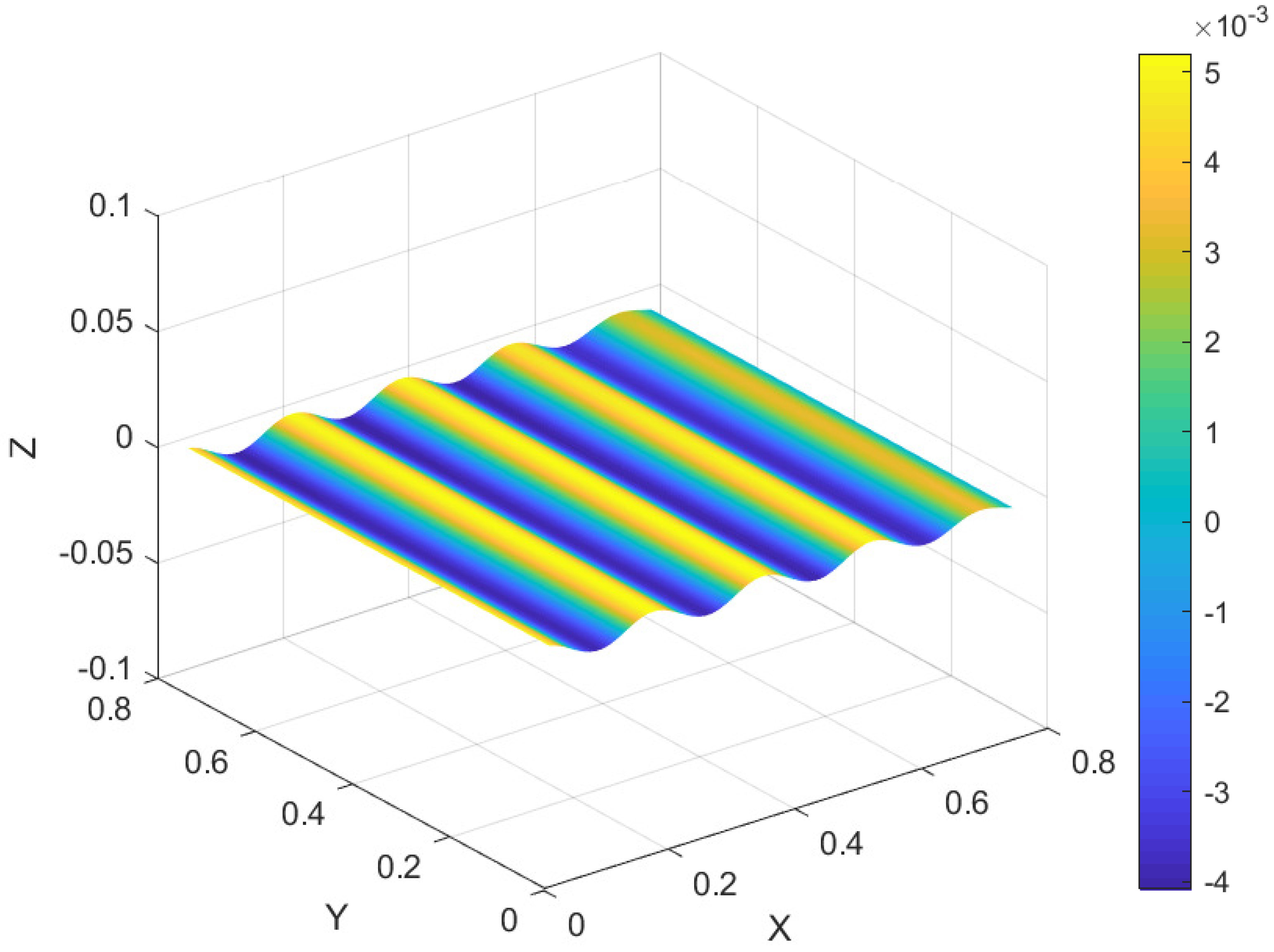
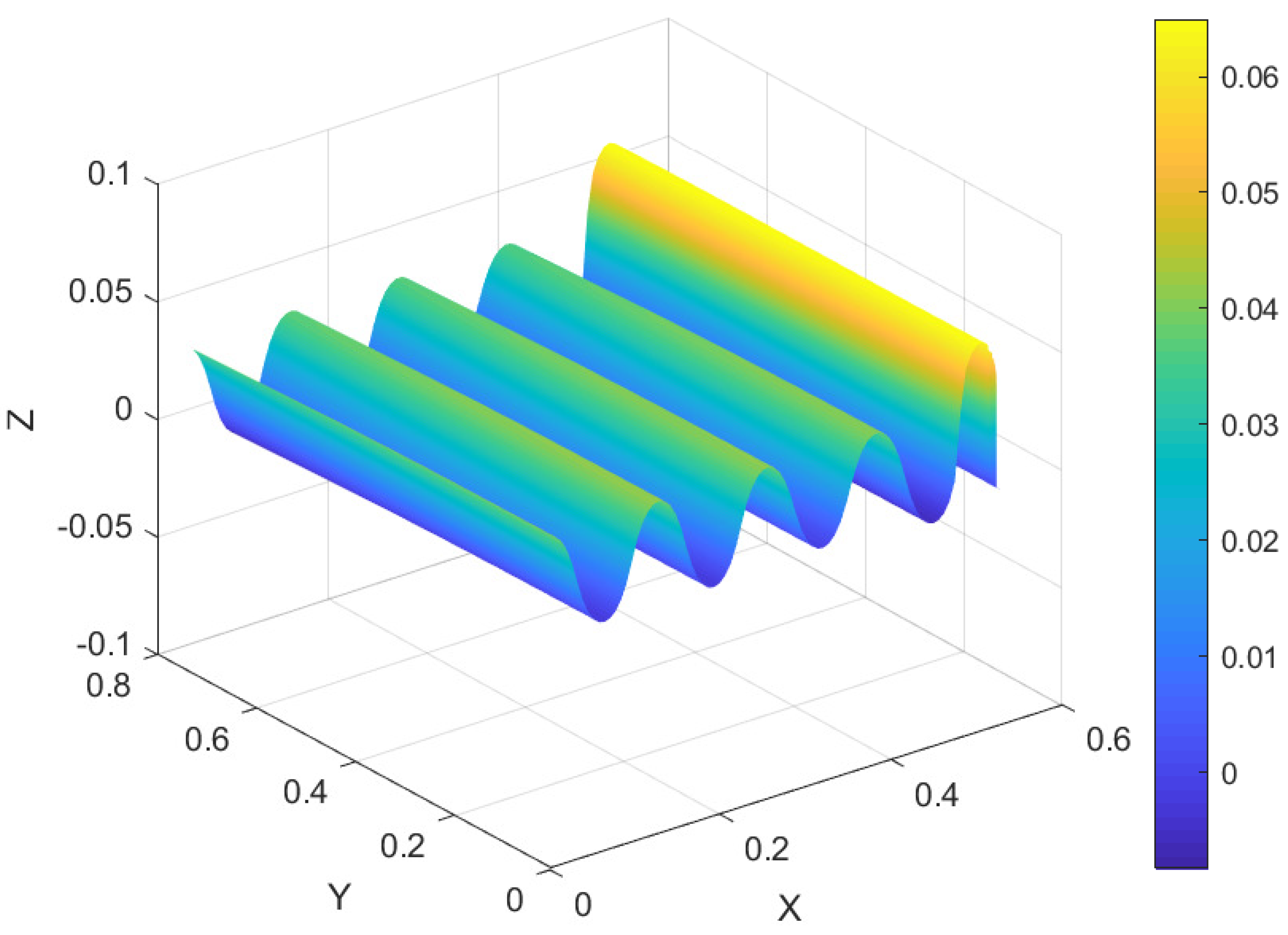
Figure 8.
Deformed of the film top surface just before the second bifurcation (ANM step 34).
6.3. Spherical Film-Substrate Under Thermal Loading
In this section, we are going to study film/substrate systems with a spherical curvature in the case of a thermo-mechanical shrinkage of its compliant core. The details of the continuation algorithm ANM used to study thermo-mechanical problems has been presented in Section 4. In [3], Xu et al. have presented an analytical model, experimental results, and numerical results. The numerical results have been obtained with the commercial software ABAQUS using both Riks method and the pseudo dynamic method. In order to characterize surface morphological pattern formation of core-shell spheres upon shrinkage of core, Xu et al. have introduced the relevant parameter where (resp. ) is the substrate (resp. film) Young’s modulus, R the radius of the sphere (, including the film thickness), and the thickness of the film ().
Figure 9 is a plot of the mesh of one eighth of the whole spherical film/substrate system (three symmetry planes are used to obtain the whole spherical structure). We can see the tetrahedron geometry of the mesh and the presence of smaller element within the film part of the mesh. The spherical film-substrate geometry has been meshed with two elements in the film thickness, an average elements length and consists in 164528 tetrahedra (689358 degrees of freedom). We choose four different values of the parameter (0.2, 2.6, 4.9, 21.2), and, the mesh is the same for the four parameters.
Let us first make the numerical simulation for . Figure 10 is the plot of the maximum normalized deflection versus the thermal loading parameter . We can observe two limit or turning points, the bifurcation curve being subcritical: the first one is close to step 10, and the second close to step 40. Then, close to step 100, another bifurcation happens and the curve is going backward. The ANM continuation does not allow to jump on another probable existing branch: future research will be done to solve this lack. Figure 11 shows the deformation (normalized deflection) for an half sphere at the steps 10, 34, 50, and 80. As in [3], we can observe isolated dimples, with a greater localization when deflection amplitude increased.
Second, let us now consider the numerical simulation for . Figure 12 is the plot of the maximum normalized deflection versus the thermal loading parameter . We can observe first a limit or turning point, the bifurcation being weakly subcritical. We can observe small back-and-forth motions and the ANM continuation still goes on. Figure 13 shows the deformation (normalized deflection) for an half sphere, exhibiting buckyball deformation patterns.
Third, let us consider the case of . Figure 14 is the plot of the maximum normalized deflection versus the thermal loading parameter . The first bifurcation appears close to step 10 and turns out to be supercritical. After, the curve is showing zigzag and the progression slows down. For Figure 15 we can observe a periodicity in the pattern, and a transition between buckyball and a symmetry breaking of buckyball pattern, around step 120 (the deflection amplitude of some dimples decreases).
Finally, let us consider . Figure 16 is the plot of the maximum normalized deflection versus the thermal loading parameter . The first bifurcation is also supercritical as previously, and appears close to step 10. Then the bifurcation curve behavior is almost linear and reaches greater thermal loading values than in the previous case. Figure 17, we can observe a smaller periodicity in the patter and also a transition between buckyball and a symmetry breaking of buckyball pattern.
7. Conclusions
In this paper, we have presented a new implementation of the Asymptotic Numerical Method within the user-friendly finite element environment FreeFem++. ANM continuation method, based on a perturbation technique, has proven to be a very efficient technique for the numerical simulation of nonlinear instability problems.The ANM has been previously implemented in FORTRAN, Matlab, and C++ to solve various problems of fluid or solid mechanics.
On the one hand, its high level Design Specific Language dedicated to variational formulations and finite elements makes it easier to write scripts for solving nonlinear solid or fluid mechanics problems using ANM. On the other hand, this new numerical tool written in FreeFem++ will be very helpful for new developments, like those concerning convergence acceleration [34] or multiscale finite elements [45,46].
A first computation using the new developed FreeFem++ code, consisting in a cantilever (Saint Venant-Kirchhoff material) submitted to a vertical surface force, where geometrical nonlinearities are taken into account, has shown a very good comparison with the commercial software Abaqus. The two other applications concern film/substrate systems. The first case is the study of a planar film/substrate system subjected to axial compression, and the second case is a spherical film/substrate system subjected to the thermo-mechanical shrinkage of its core. Both film/substrate applications have demonstrated the efficiency of the implementation of ANM in FreeFem++ for the following of equilibrium paths when solving solid mechanical problems.
In the present state, the achieved implementation concerns geometrically nonlinear elasticity, but the extension to other models of solid and fluid mechanics seems rather easy. Among the contributions of FreeFem++, let’s mention the treatment of multiphysics modelings or of large scale problems thanks to its interface with the PETSc library. In this paper, the MPI/MUMPS parallel version has been applied.
Finally, a supplementary article shows the details of the FreeFEM++ implementations.
Author Contributions
For research articles with several authors, a short paragraph specifying their individual contributions must be provided. The following statements should be used “Conceptualization, P.V., M.P., and F.H.; methodology, P.V., M.P., M.B., A.C.; software, F.H. and P.V.; validation, P.V., F.X. ; formal analysis, M.P., F.H. and P.V.; investigation, ; resources, P.V.; data curation, P.V.; writing—original draft preparation, P.V.; writing—review and editing, P.V.; visualization, H.A.; supervision, M.P.; project administration, X.X.; funding acquisition, M.P and F.X. All authors have read and agreed to the published version of the manuscript.
Funding
This work was supported by the French State through the program "Investment in the future" operated by the National Research Agency (ANR) and referenced by ANR-11-LABX-0008-01 (LabEx DAMAS). Fan Xu acknowledges financial supports from the National Natural Science Foundation of China (Grants No. 12425204, 12122204, and 12372096), Shanghai Pilot Program for Basic Research-Fudan University (Grant No. 21TQ1400100-21TQ010), and Shanghai Municipal Education Commission (Grant No. 24KXZNA14).
Data Availability Statement
Data are contained within the article.
Acknowledgments
The authors thanks the EXPLOR HPC center for computational ressources
Conflicts of Interest
The authors declare no conflicts of interest.
Appendix A. FreeFEM++ Implementation of ANM When the ANM Order Is Greater than 2
Here we are going to present the implementation of the ANM order loop. The current order is p.
Let us compute :
- unl[] = Kt^-1*Fnlu[];
- lambda[p] = -lambda[1]*(unl[]’*u[1][]);
- u[p][] = lambda[p]/lambda[1]*u[1][]+unl[];
Then, we compute :
- [Sxx[p],Syy[p],Szz[p],deuxSxy[p],deuxSxz[p],deuxSyz[p]] =
- DL*(GammaL(u[p],v[p],w[p])+
- 2*GammaNL(u[0],v[0],w[0],u[p],v[p],w[p]))
- +[Snlxx,Snlyy,Snlzz,deuxSnlxy,deuxSnlxz,deuxSnlyz];
a loop is necessary to compute for the next ANM order;
- [Snlxx,Snlyy,Snlzz,deuxSnlxy,deuxSnlxz,deuxSnlyz] =
- [0.,0.,0.,0.,0.,0.];
- for (int ir=1;ir<(p+1);ir++)
- {
- [Snlxx,Snlyy,Snlzz,deuxSnlxy,deuxSnlxz,deuxSnlyz] =
- [Snlxx,Snlyy,Snlzz,deuxSnlxy,deuxSnlxz,deuxSnlyz]
- + GammaNL(u[p+1-ir],v[p+1-ir],w[p+1-ir],u[ir],v[ir],w[ir]);
- }
- [Snlxx,Snlyy,Snlzz,deuxSnlxy,deuxSnlxz,deuxSnlyz] = D*
- [Snlxx,Snlyy,Snlzz,deuxSnlxy,deuxSnlxz,deuxSnlyz];
Let us notice that is overwritten at each order.
It is now possible to assemble the nonlinear second member :
- Vh [Fnlutmp,Fnlvtmp,Fnlwtmp];
- [Fnlu,Fnlv,Fnlw] = [0.,0.,0.];
- [Fnlutmp,Fnlvtmp,Fnlwtmp] = [0.,0.,0.];
- for (int ir=1;ir<(p+1);ir++)
- {
- varf PbFnla ([utmp,vtmp,wtmp],[uuu,vvv,www]) = - int3d(Th3D)
- ( (dGammaNL(u[p+1-ir],v[p+1-ir],w[p+1-ir],uuu,vvv,www))’*
- ([Sxx[ir],Syy[ir],Szz[ir],deuxSxy[ir],deuxSxz[ir],deuxSyz[ir]
- ))
- + on(lencasmid,utmp=0.,vtmp=0.,wtmp=0.);
- Fnlutmp[] = PbFnla(0,Vh);
- Fnlu[] = Fnlu[] + Fnlutmp[];
- }
- Vh [Fnlutmp,Fnlvtmp,Fnlwtmp];
- Fnlutmp[] = 0.0;
- varf PbFnlc ([utmp,vtmp,wtmp],[uuu,vvv,www]) =
- - int3d(Th3D) ( (dGamma(u[0],v[0],w[0],uuu,vvv,www))’*
- ([Snlxx,Snlyy,Snlzz,deuxSnlxy,deuxSnlxz,deuxSnlyz]) )
- + on(lencasmid,utmp=0.,vtmp=0.,wtmp=0.);
- [Fnlutmp,Fnlvtmp,Fnlwtmp] = [0.,0.,0.];
- Fnlutmp[] = PbFnlc(0,Vh);
- Fnlu[] = Fnlu[] + Fnlutmp[];
Appendix B. Newton-Raphson Continuation and Newton-Riks Correction Algorithms
The algorithm (A1) (resp. A2) gives the several steps of the classical Newton-Raphson (resp. Newton-Riks correction) algorithm.
| Algorithm A1 Algorithm Newton-Raphson Prediction |
|
| Algorithm A2 Algorithm Newton-Riks correcions |
|
References
- Wong, W.; Pellegrino, S. Wrinkled membranes III: numerical simulations. Journal of Mechanics of Materials and Structures 2006, 1, 63–95. [Google Scholar] [CrossRef]
- Chen, X.; Hutchinson, J.W. Herringbone buckling patterns of compressed thin films on compliant substrates. Journal of Applied Mechanics 2004, 71, 597–603. [Google Scholar] [CrossRef]
- Xu, F.; Zhao, S.; Conghua, L.; Potier-Ferry, M. Pattern selection in core-shell spheres. Journal of the Mechanics and Physics of Solids (2020) 103892, 137. [CrossRef]
- Tian, H.; Potier-Ferry, M.; Abed-Meraim, F. Buckling and wrinkling of thin membranes by using a numerical solver based on multivariate Taylor series. International Journal of Solids and Structures 2021, 230, 111165. [Google Scholar] [CrossRef]
- Rodriguez, J.; Rio, G.; Cadou, J.M.; Troufflard, J. Numerical study of dynamic relaxation with kinetic damping applied to inflatable fabric structures with extensions for 3D solid element and non-linear behavior. Thin-Walled Structures 2011, 49, 1468–1474. [Google Scholar] [CrossRef]
- Taylor, M.; Bertoldi, K.; Steigmann, D.J. Spatial resolution of wrinkle patterns in thin elastic sheets at finite strain. Journal of the Mechanics and Physics of Solids 2014, 62, 163–180. [Google Scholar] [CrossRef]
- Thompson, J.M.T.; Walker, A.C. The non-linear perturbation analysis of discrete structural systems. International Journal of Solids and Structures 1968, 4, 757–768. [Google Scholar] [CrossRef]
- Cochelin, B. A path following technique via an asymptotic-numerical method. Computers and Structures 1994, 53(5), 1181–1192. [Google Scholar] [CrossRef]
- Cochelin, B.; Damil, N.; Potier-Ferry, M. The asymptotic numerical method : an efficient technique for non linear structural mechanics. Revue Européenne des Eléments Finis 1994, 3, 281–297. [Google Scholar] [CrossRef]
- Cochelin, B.; Damil, N.; Potier-Ferry, M. Asymptotic-numerical methods and Padé approximants for non linear elastic structure. International journal of Numerical Methods in Engineering 1994, 37, 1187–1213. [Google Scholar] [CrossRef]
- Azrar, L.; Cochelin, B.; Damil, N.; Potier-Ferry, M. An asymptotic-numerical method to compute the postbuckling behaviour of elastic plates and shells. International Journal for Numerical Methods in Engineering 1993, 36, 1251–1277. [Google Scholar] [CrossRef]
- Tri, A.; Cochelin, B.; Potier-Ferry, M. Résolution des équations de Navier-Stokes et Détection des bifurcations stationnaires par une Méthode Asymptotique-Numérique. Revue Européenne des éléments Finis 1996, 5, 415–442. [Google Scholar] [CrossRef]
- Elhage-Hussein, A.; Damil, N.; Potier-Ferry, M. An asymptotic numerical algorithm for frictionless contact problems. Revue Européenne des éléments Finis 1998, 7, 119–130. [Google Scholar] [CrossRef]
- Zahrouni, H.; Cochelin, B.; Potier-Ferry, M. Computing finite rotations of shells by an asymptotic-numerical method. Computer Methods in Applied Mechanics and Engineering 1999, 175, 71–85. [Google Scholar] [CrossRef]
- Cadou, J.M.; Potier-Ferry, M.; Cochelin, B. A numerical method for the computation of bifurcation points in fluid mechanics. European Journal of Mechanics - B/Fluids 2006, 25, 234–254. [Google Scholar] [CrossRef]
- Aggoune, W.; Zahrouni, H.; Potier-Ferry, M. Asymptotic numerical methods for unilateral contact. International Journal for Numerical Methods in Engineering 2006, 68, 605–631. [Google Scholar] [CrossRef]
- Cong, Y.; Nezamabadi, S.; Zahrouni, H.; Yvonnet, J. Multiscale computational homogenization of heterogeneous shells at small strains with extensions to finite displacements and buckling. International Journal for Numerical Methods in Engineering 2015, 104, 235–259. [Google Scholar] [CrossRef]
- Riks, E. An incremental approach to the solution of snapping and buckling problems. International Journal of Solids and Structures 1979, 15, 529–551. [Google Scholar] [CrossRef]
- R. Arquier, B. R. Arquier, B. Cochelin, C. Manlab, http://manlab.lma.cnrs-mrs.fr/.
- Lejeune, A.; Béchet, F.; Boudaoud, H.; Mathieu, N.; Potier-Ferry, M. Object-oriented design to automate a high order non-linear solver based on asymptotic numerical method. Advances in Engineering Software 2012, 48, 70–88. [Google Scholar] [CrossRef]
- Guevel, Y.; Allain, T.; Girault, G.; Cadou, J.M. Numerical bifurcation analysis for 3-dimensional sudden expansion fluid dynamic problem. International Journal for Numerical Methods in Fluids 2018, 87, 1–26. [Google Scholar] [CrossRef]
- Hecht, F. New development in FreeFem++. Journal of Numerical Mathematics 2012, 20, 251–265. [Google Scholar] [CrossRef]
- Hecht, F.; Ventura, P.; Dufilié, P. Original coupled FEM/BIE numerical model for analyzing infinite periodic surface acoustic wave transducers. Journal of Computational Physics 2013, 246, 265–274. [Google Scholar] [CrossRef]
- Hecht, F.; Pironneau, O. An energy stable monolithic Eulerian fluid-structure finite element method. International Journal for Numerical Methods in Fluids 2017, 85, 430–446. [Google Scholar] [CrossRef]
- Xu, F.; Potier-Ferry, M.; Belouettar, S.; Cong, Y. 3D finite element modeling for instabilities in thin films on soft substrates. International Journal of Solids and Structures 2014, 51, 3619–3632. [Google Scholar] [CrossRef]
- Xu, F.; Koutsawa, Y.; Potier-Ferry, M.; Belouettar, S. Instabilities in thin films on hyperelastic substrates by 3D finite elements. International Journal of Solids and Structures 2015, 69-70, 71–85. [Google Scholar] [CrossRef]
- Cochelin, B.; Damil, N.; Potier-Ferry, M. Méthode asymptotique numérique; Hermès-Lavoisier, 2007.
- Potier-Ferry, M. Asymptotic numerical method for hyperelasticity and elastoplasticity: a review. Proceeding of the Royal Society 2024, 480. [Google Scholar] [CrossRef]
- Gourdon, X. Analyse; Ellipse, 2020.
- Berger, M.S. Nonlinearity and functional analysis: lectures on nonlinear problems in mathematical analysis. Academic press, New York 1977, 74. [Google Scholar]
- Berger, M.S. Method of Lyapunov and Schmidt in the study of non-linear equation and their further development. Russian mathematical surveys 1962, 17. [Google Scholar]
- Mottaqui, H.; Braikat, B.; Damil, N. Discussion about parameterization in the asymptotic numerical method: application to nonlinear elastic shells. Computer Methods in Applied Mechanics and Engineering 2010, 199, 1701–1709. [Google Scholar] [CrossRef]
- Lahmam, H.; Cadou, J.M.; Zahrouni, H.; Damil, N.; Potier-Ferry, M. High-order predictor–corrector algorithms. International Journal for Numerical Methods in Engineering 2002, 55, 685–704. [Google Scholar] [CrossRef]
- Ventura, P.; Potier-Ferry, M.; Zahrouni, H. A secure version of asymptotic numerical method via convergence acceleration. Comptes Rendus Mécaniques 2020, 348, 361–374. [Google Scholar] [CrossRef]
- Assidi, M.; Zahrouni, H.; Damil, N.; Potier-Ferry, M. Regularization and perturbation technique to solve plasticity problems. International Journal of Material Forming 2009, 2, 1–14. [Google Scholar] [CrossRef]
- El Kihal, C.; Askour, O.; Belaasilia, Y.; Hamdaoui, A.; Braikat, B.; Damil, N.; Potier-Ferry, M. Asymptotic numerical method for finite plasticity. Finite Elements in Analysis and Design 2022, 206, 103759. [Google Scholar] [CrossRef]
- Zahrouni, H. Méthode Asymptotique Numérique pour les coques en grande rotation. PhD thesis, Université de Lorraine, 1998.
- Bowden, N.; Brittain, S.; Evans, A.G.; Hutchinson, J.W.; Whitesides, G.M. Spontaneous formation of ordered structures in thin films of metals supported on an elastomeric polymer. Nature 1998, 393, 146–149. [Google Scholar] [CrossRef]
- Bowden, N.; Huck, W.; Paul, K.; Whitesides, G.M. The control formation of ordered, sinusoidal structures by plasma oxidation of an elastometric polymer. Applied Physics Letters 1999, 75(17), 2557–2559. [Google Scholar] [CrossRef]
- Wang, S.; Song, J.; Kim, D.H.; Huang, Y.; Rogers, J.A. Local versus global buckling of thin films on elastometric substrates. Applied Physics Letters, 0231. [Google Scholar] [CrossRef]
- Howarter, J.; Stafford, C. Instabilities as a measurement tool for soft materials. Soft Mater 2010, 6(22), 5661–5666. [Google Scholar] [CrossRef]
- Büchter", N.; Ramm, E.; Roehl, D. Three dimensional extension of non-linear shell formulation based on the enhanced assumed strain concept. International Journal for Numeral Methods in Engineering 1994, 37, 2551–2568. [Google Scholar] [CrossRef]
- Chen, X.; Hutchinson, J. Herringbone buckling patterns of compressed thin films on compliant substrates. Journal of Applied Mechanics 2004, 71, 597–603. [Google Scholar] [CrossRef]
- Baguet, S.; Cochelin, B. On the behaviour of the ANM continuation in the presence of bifurcation. Communication in Numerical Methods in Engineering 2003, 19, 459–471. [Google Scholar] [CrossRef]
- Feyel, F.; Chaboche, J.L. FE2 multiscale approach for modelling the elastoviscoplastic behaviour of long fibre SiC/Ti composite materials. Computer Methods in Applied Mechanics and Engineering 2000, 183, 309–330. [Google Scholar] [CrossRef]
- Nezamabadi, S.; Yvonnet, J.; Zahrouni, H.; Potier-Ferry, M. A multilevel computational strategy for microscopic and macroscopic instabilities. Computer Methods in Applied Mechanics and Engineering 2009, 198, 2099–2110. [Google Scholar] [CrossRef]
Figure 1.
Clamped beam submitted to a vertical conservative surface traction.
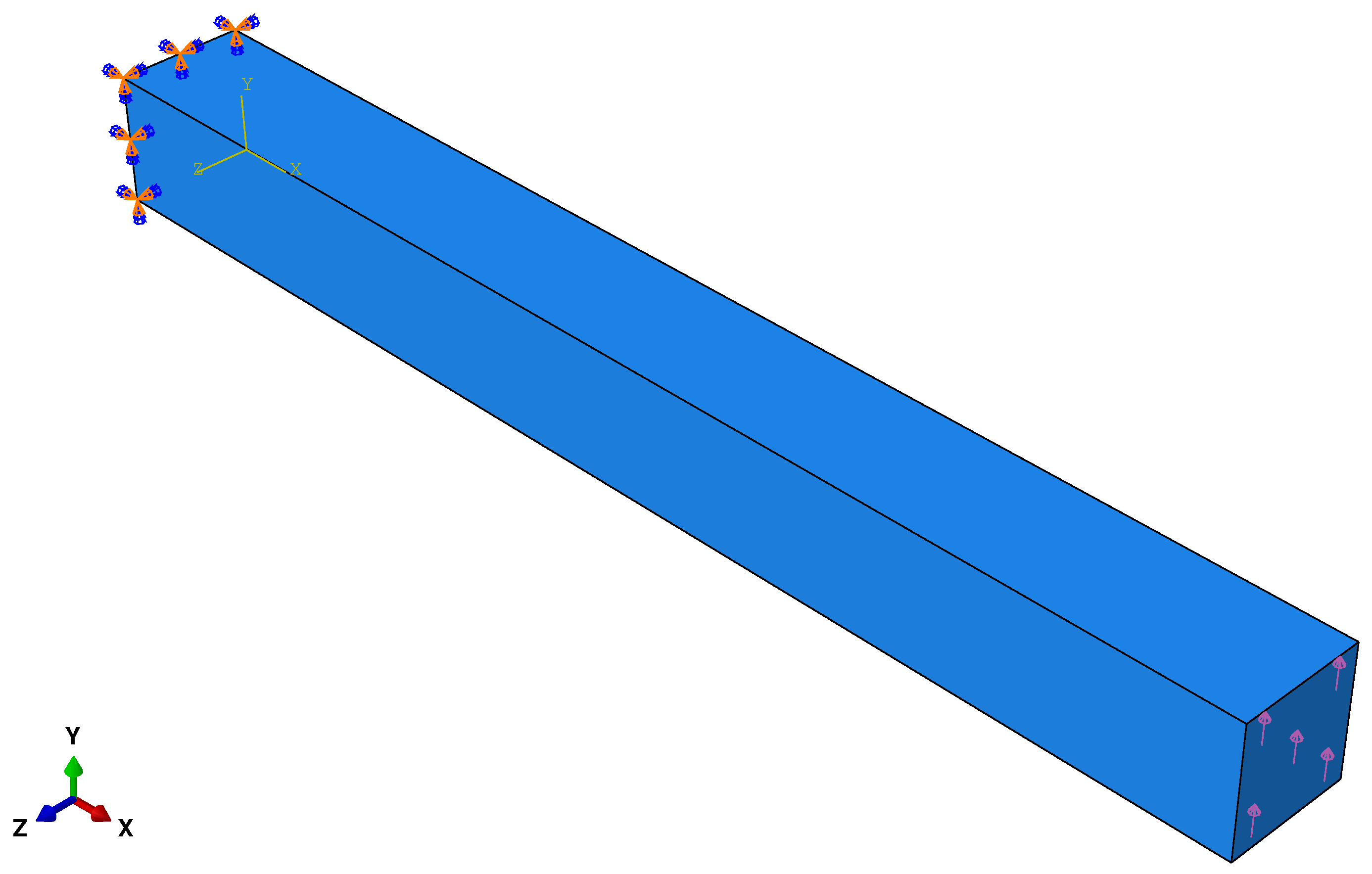
Figure 2.
Mesh of the beam using tetraedral P2 Lagrangian finite elements.
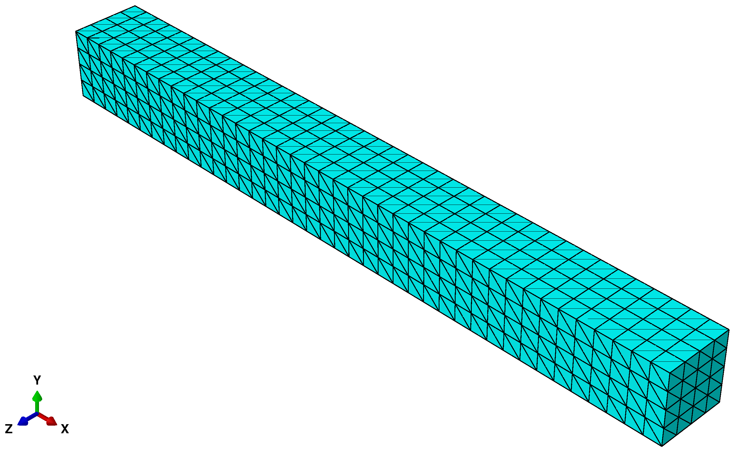
Figure 3.
Plot of versus the vertical displacement of the center of the right face. Dots mark the end of ANM steps.
Figure 3.
Plot of versus the vertical displacement of the center of the right face. Dots mark the end of ANM steps.
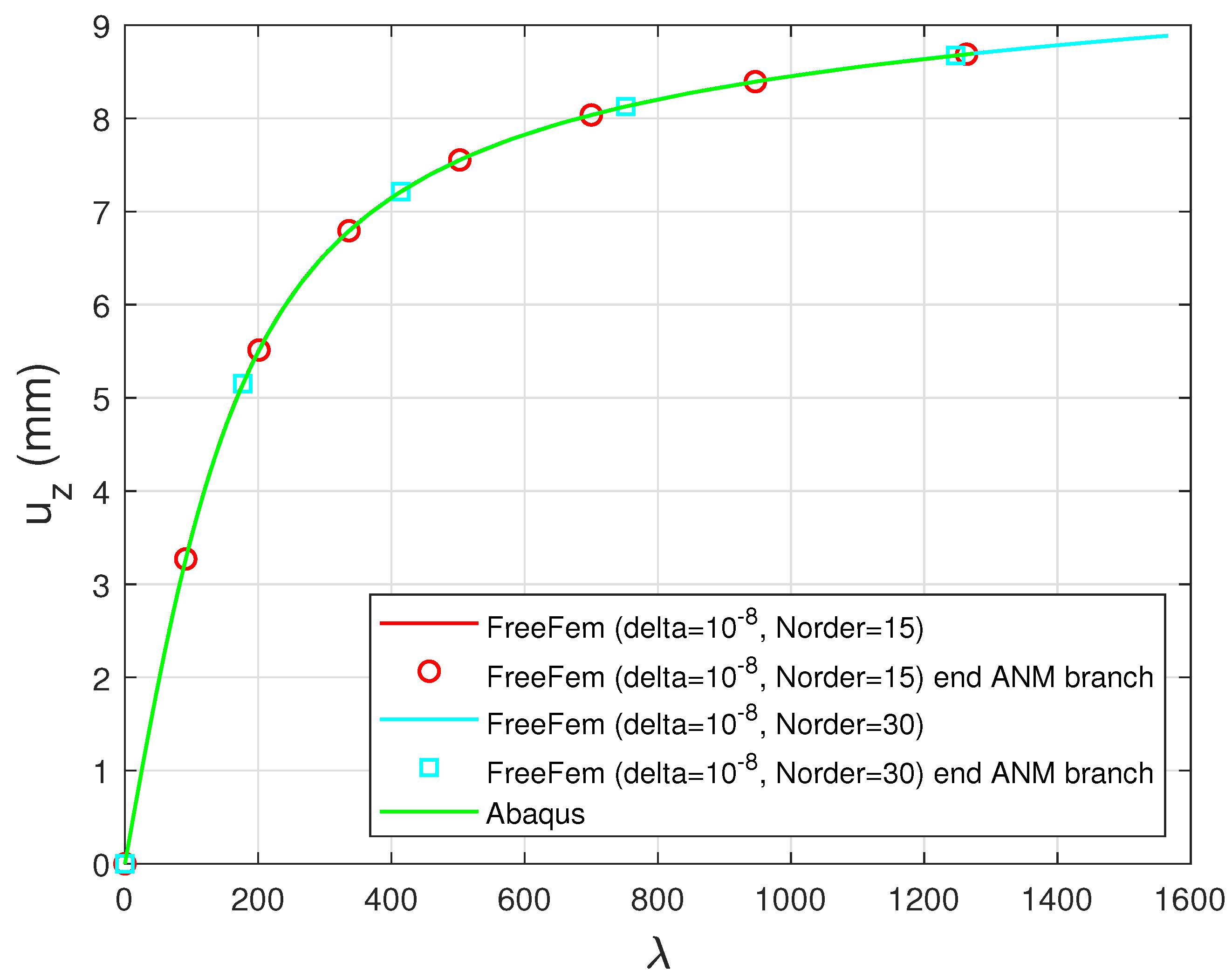
Figure 4.
Schematic of film/substrate system taking into account symmetry plane (the uniaxial force is applied of the surfaces).
Figure 4.
Schematic of film/substrate system taking into account symmetry plane (the uniaxial force is applied of the surfaces).
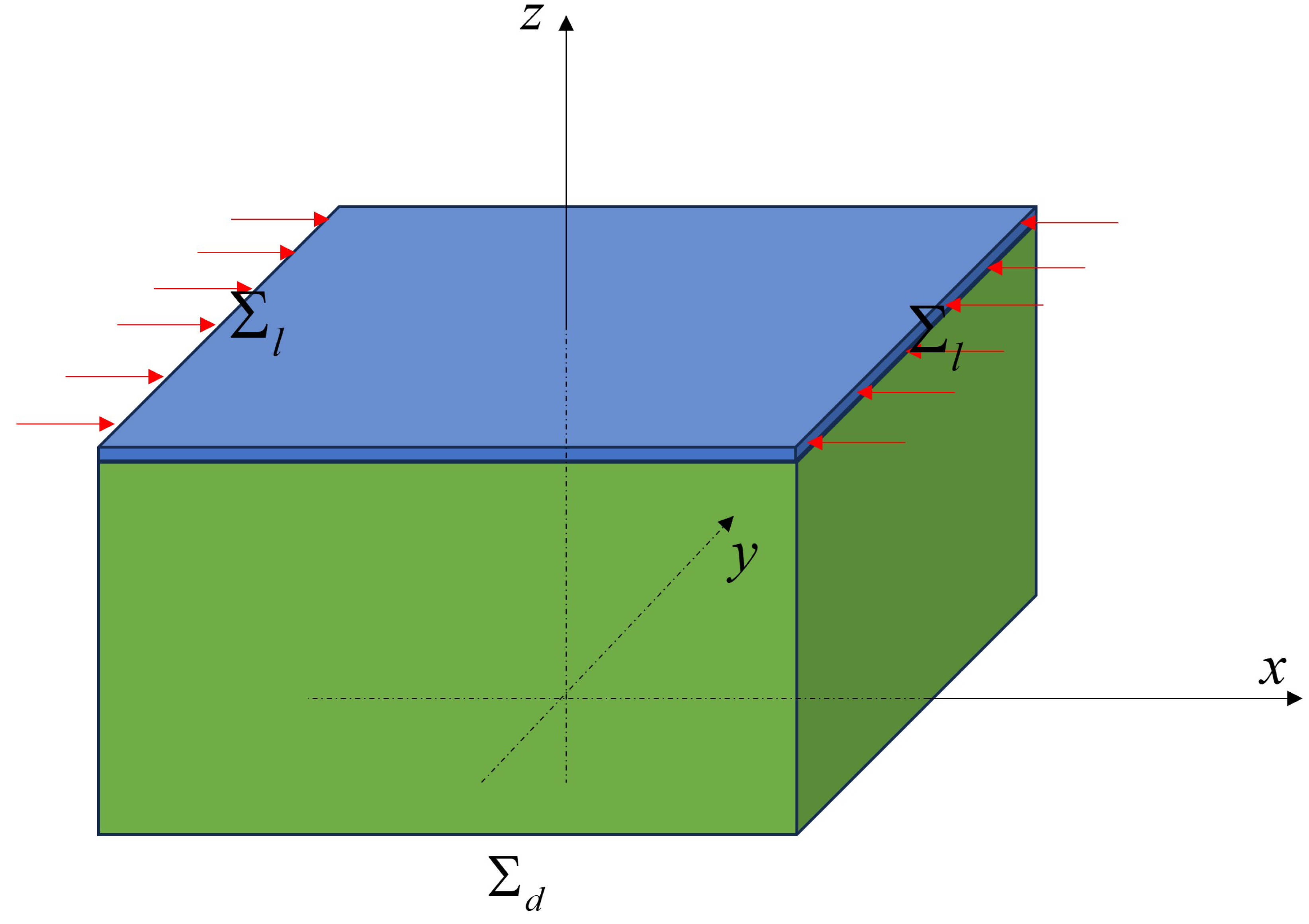
Figure 9.
3D mesh of the film/substrate system with a spherical curvature (one eight of the whole structure, using symmetry planes).
Figure 9.
3D mesh of the film/substrate system with a spherical curvature (one eight of the whole structure, using symmetry planes).
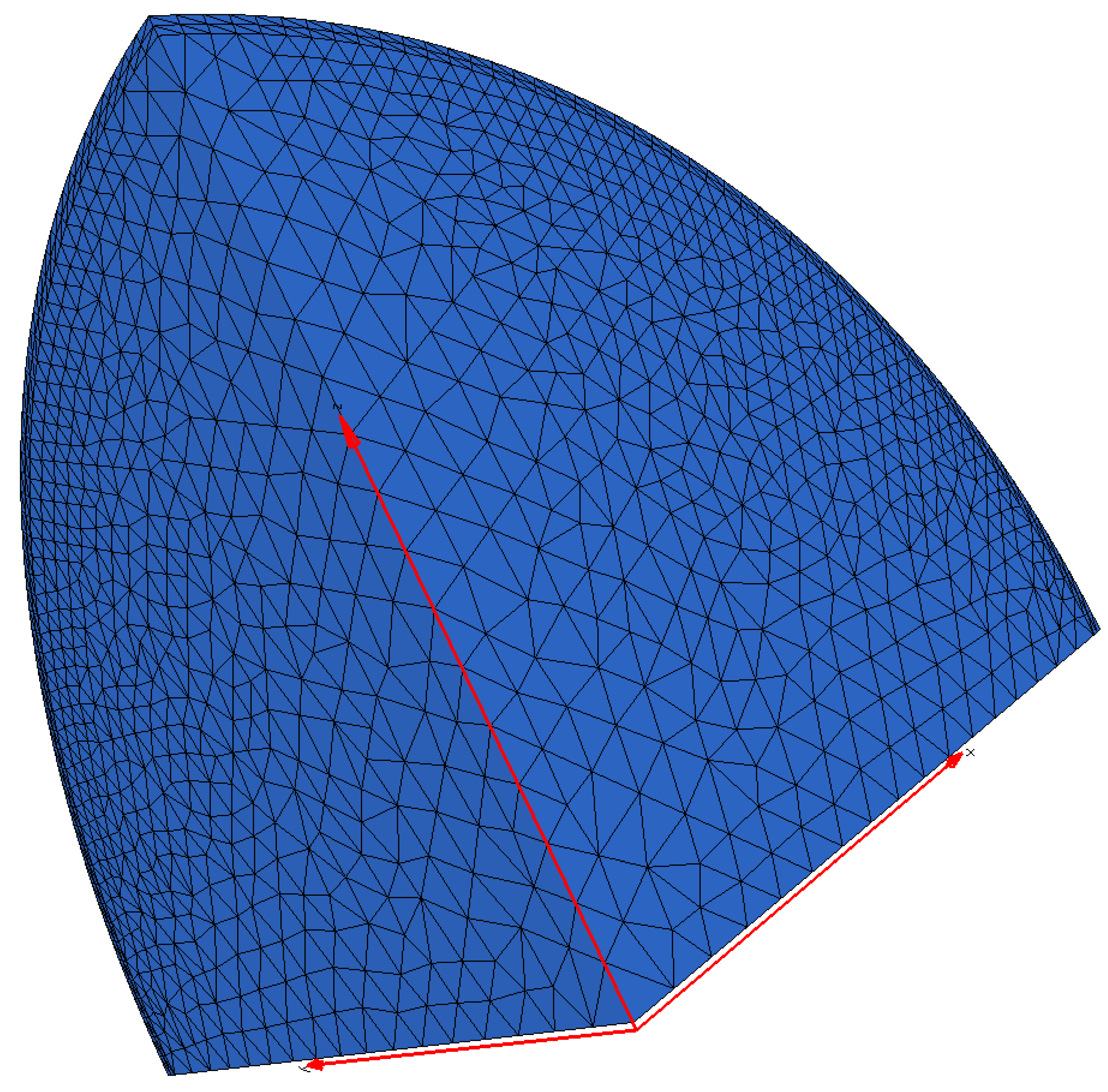
Figure 10.
Bifurcation diagram for : plot of the maximum normalized deflection versus the thermal loading parameter .
Figure 10.
Bifurcation diagram for : plot of the maximum normalized deflection versus the thermal loading parameter .
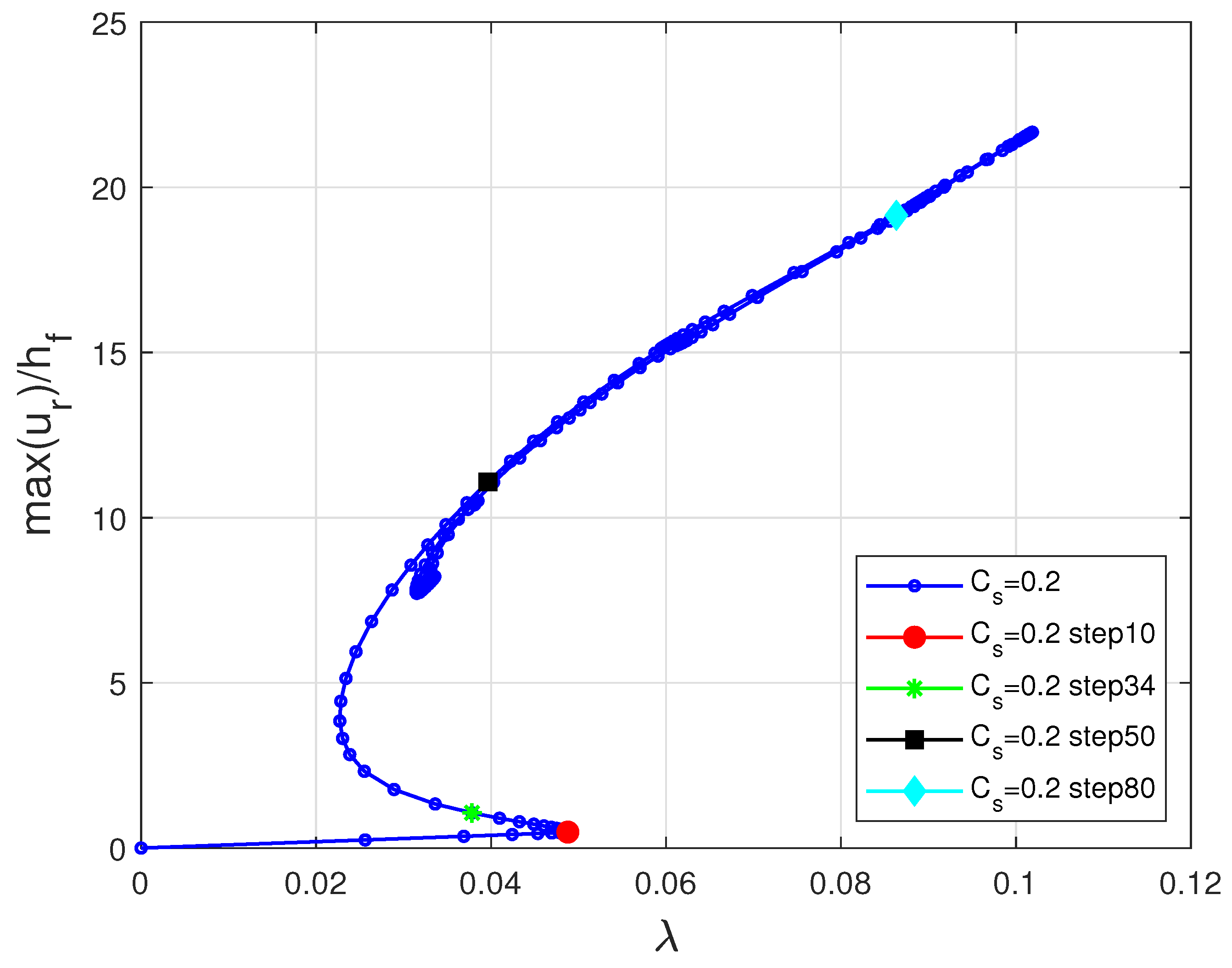
Figure 11.
Plot of the normalized deflection for , (a) step 10, (b) step 34, (c) step 50, (d) step 80.
Figure 11.
Plot of the normalized deflection for , (a) step 10, (b) step 34, (c) step 50, (d) step 80.
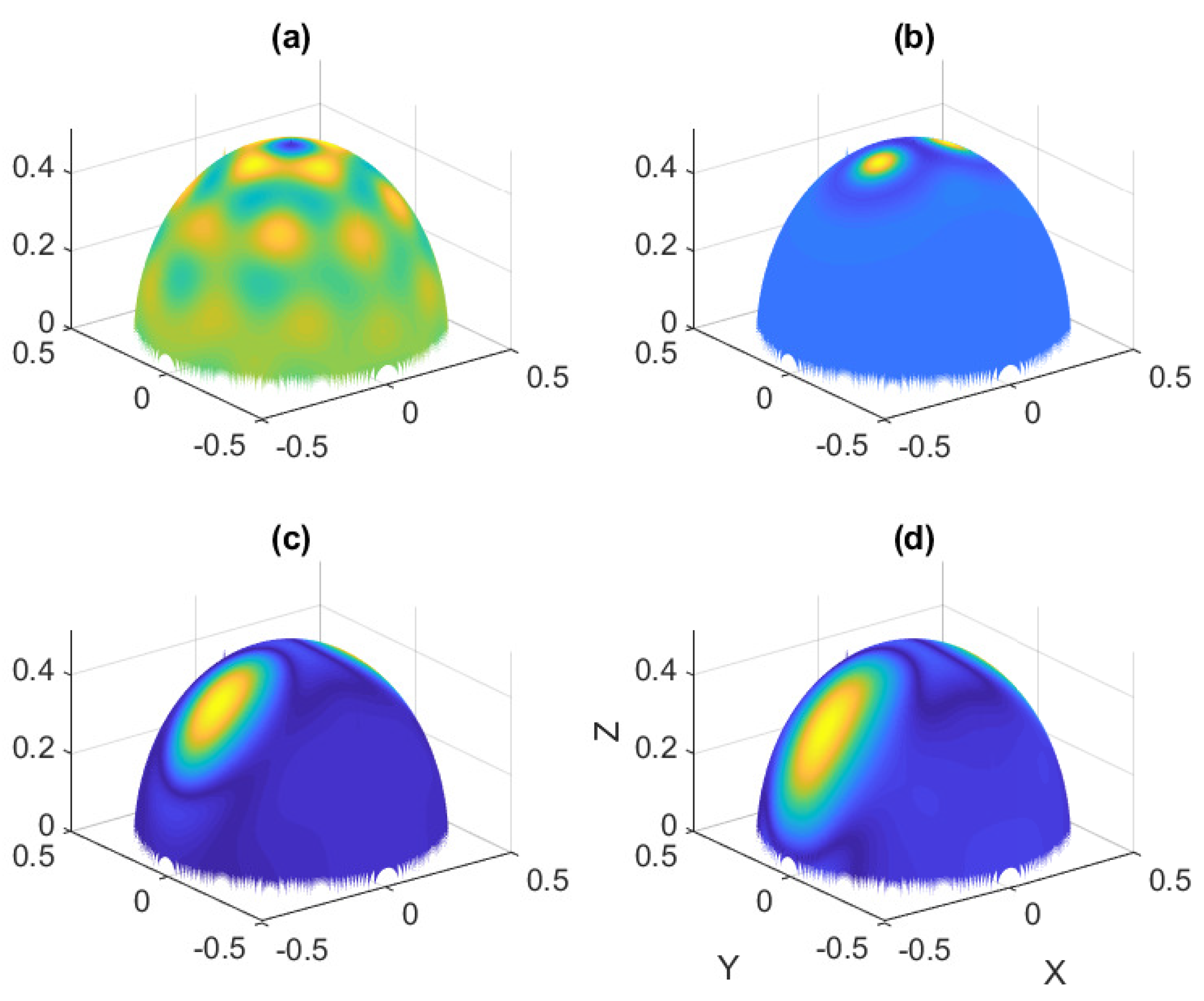
Figure 12.
Bifurcation diagram for : plot of the maximum normalized deflection versus the thermal loading parameter .
Figure 12.
Bifurcation diagram for : plot of the maximum normalized deflection versus the thermal loading parameter .
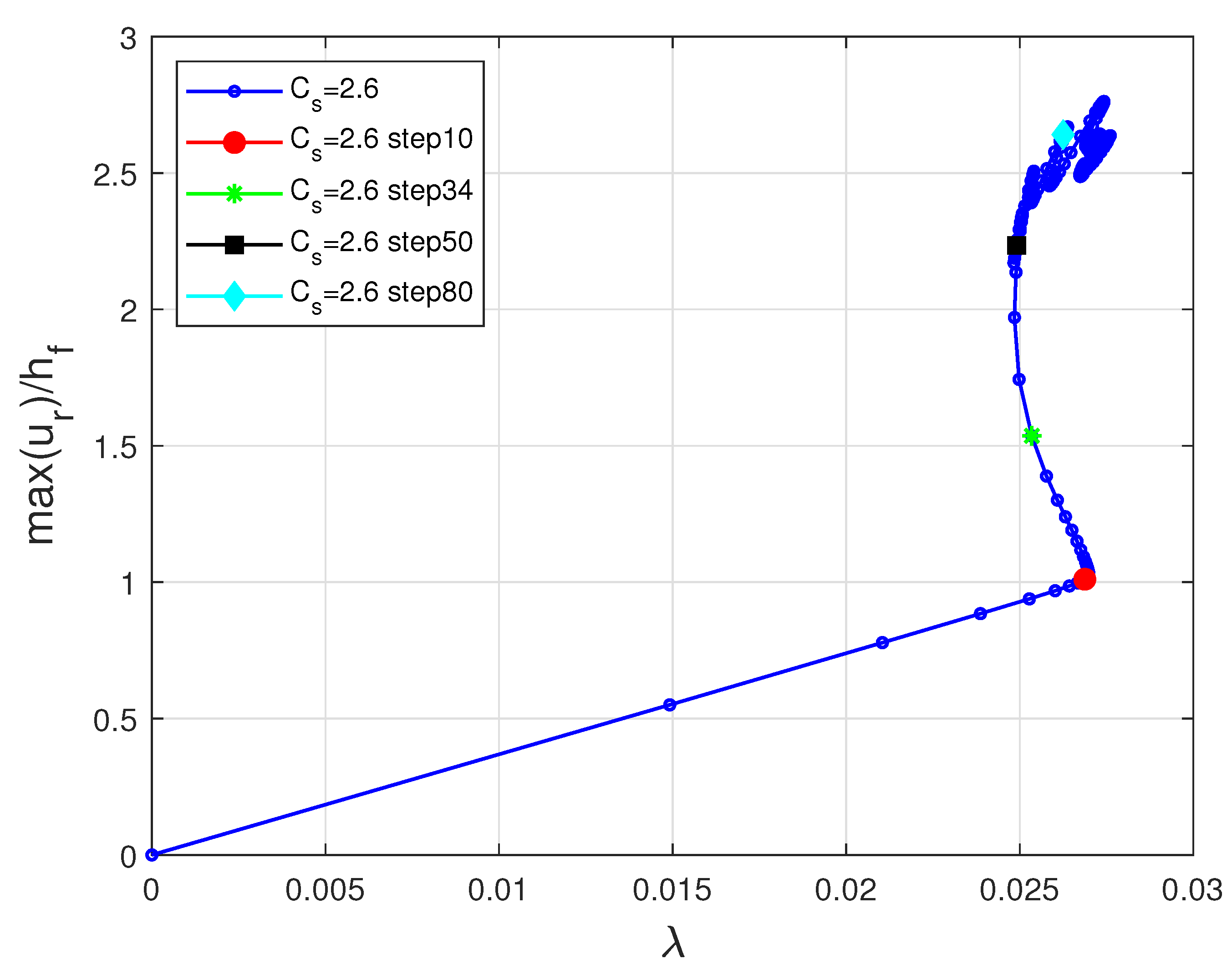
Figure 13.
Plot of the normalized deflection for . , (a) step 10, (b) step 34, (c) step 50, (d) step 80.
Figure 13.
Plot of the normalized deflection for . , (a) step 10, (b) step 34, (c) step 50, (d) step 80.
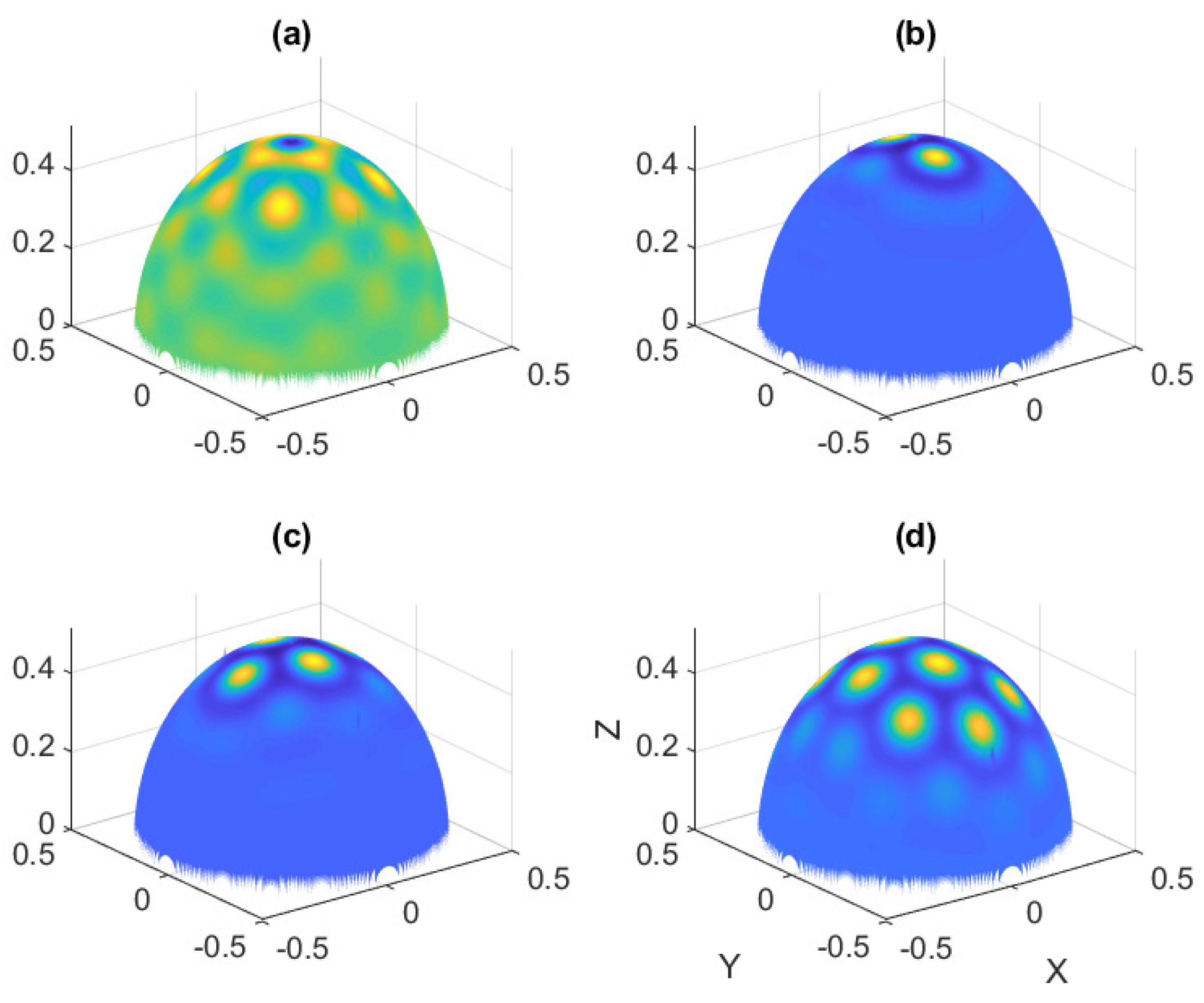
Figure 14.
Bifurcation diagram for : plot of the maximum normalized deflection versus the thermal loading parameter .
Figure 14.
Bifurcation diagram for : plot of the maximum normalized deflection versus the thermal loading parameter .
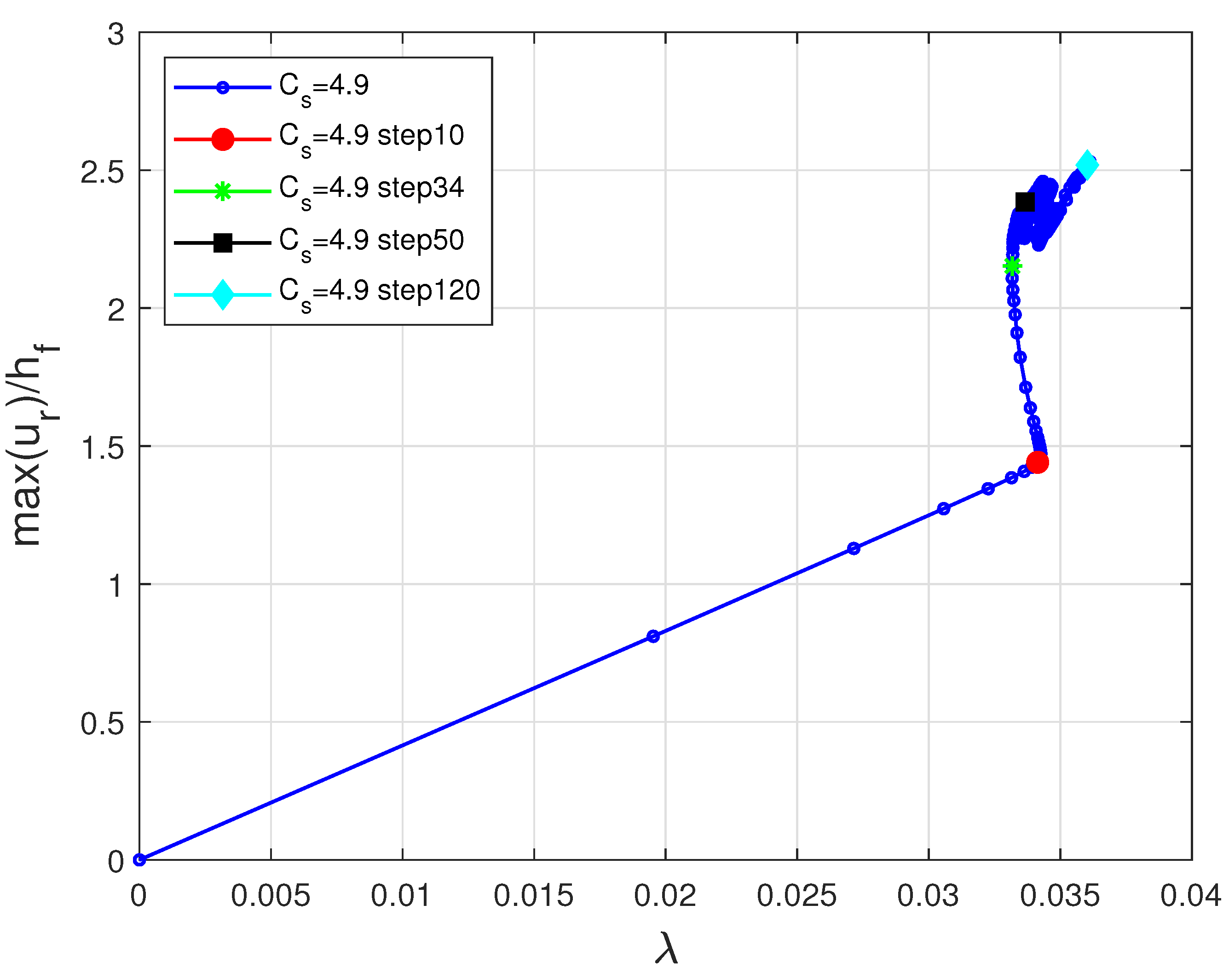
Figure 15.
Plot of the normalized deflection for , (a) step 10, (b) step 34, (c) step 50, (d) step 120.
Figure 15.
Plot of the normalized deflection for , (a) step 10, (b) step 34, (c) step 50, (d) step 120.
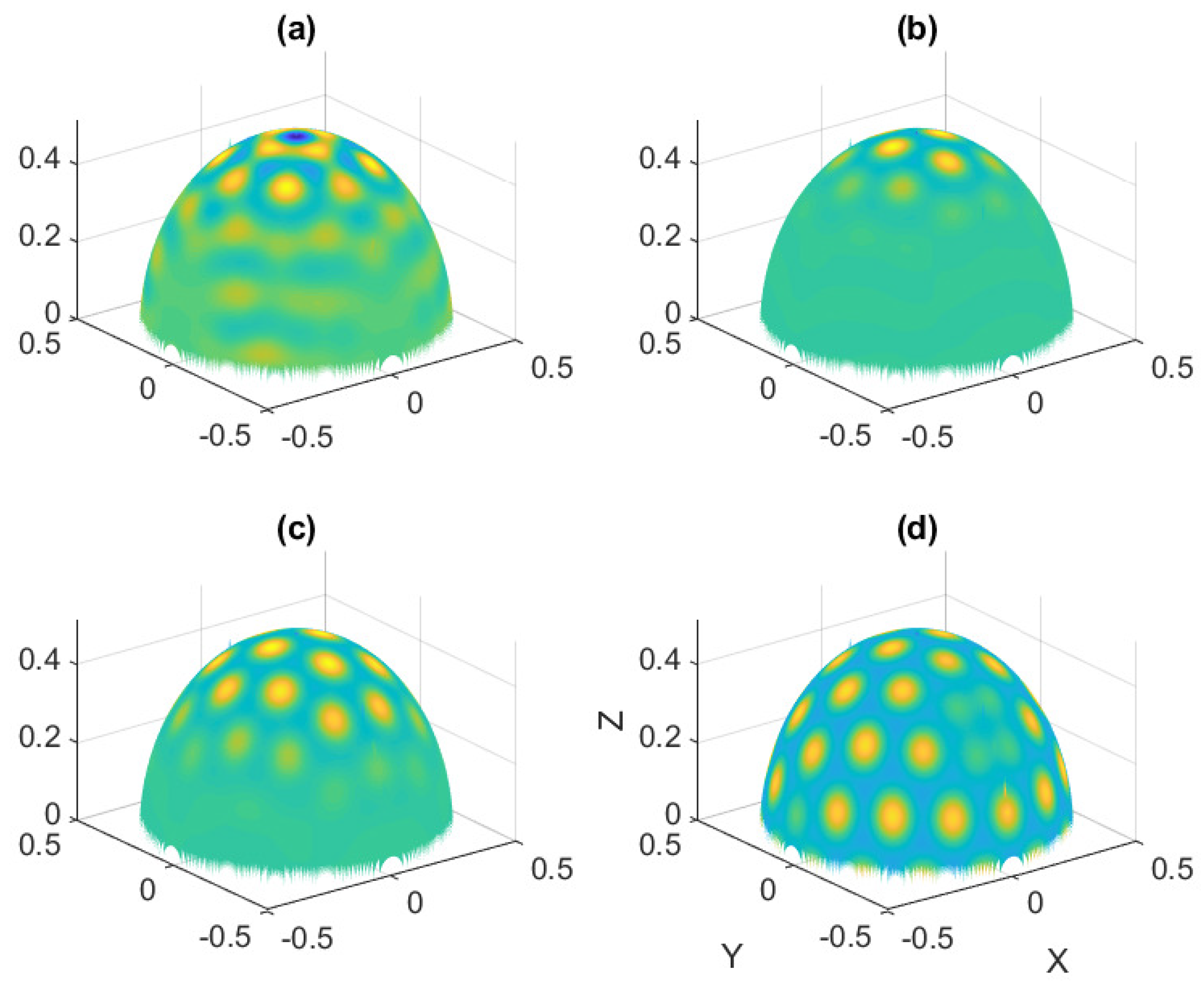
Figure 16.
Bifurcation diagram for : plot of the maximum normalized deflection versus the thermal loading parameter .
Figure 16.
Bifurcation diagram for : plot of the maximum normalized deflection versus the thermal loading parameter .
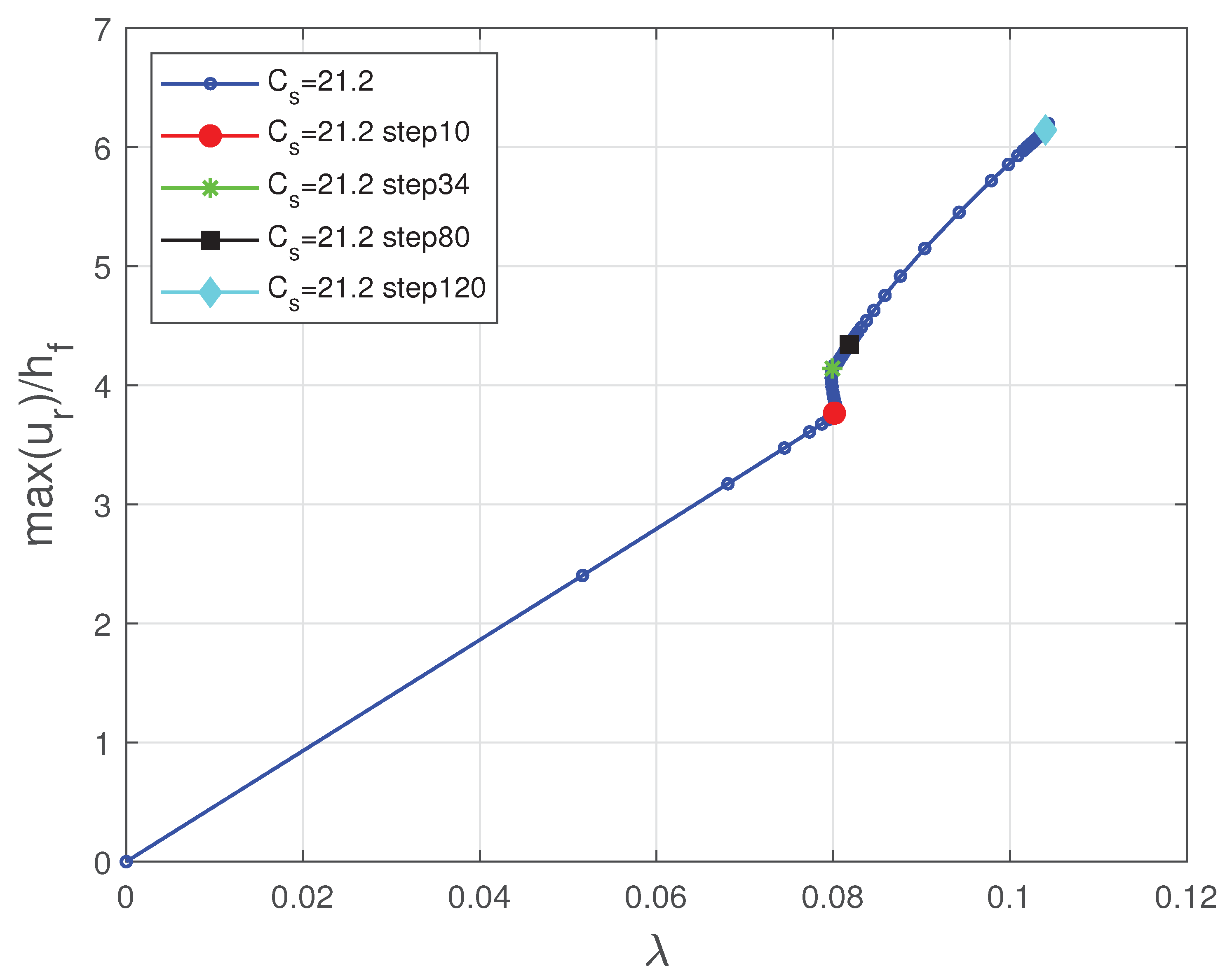
Figure 17.
Plot of the normalized deflection for , (a) step 10, (b) step 34, (c) step 80, (d) step 120.
Figure 17.
Plot of the normalized deflection for , (a) step 10, (b) step 34, (c) step 80, (d) step 120.
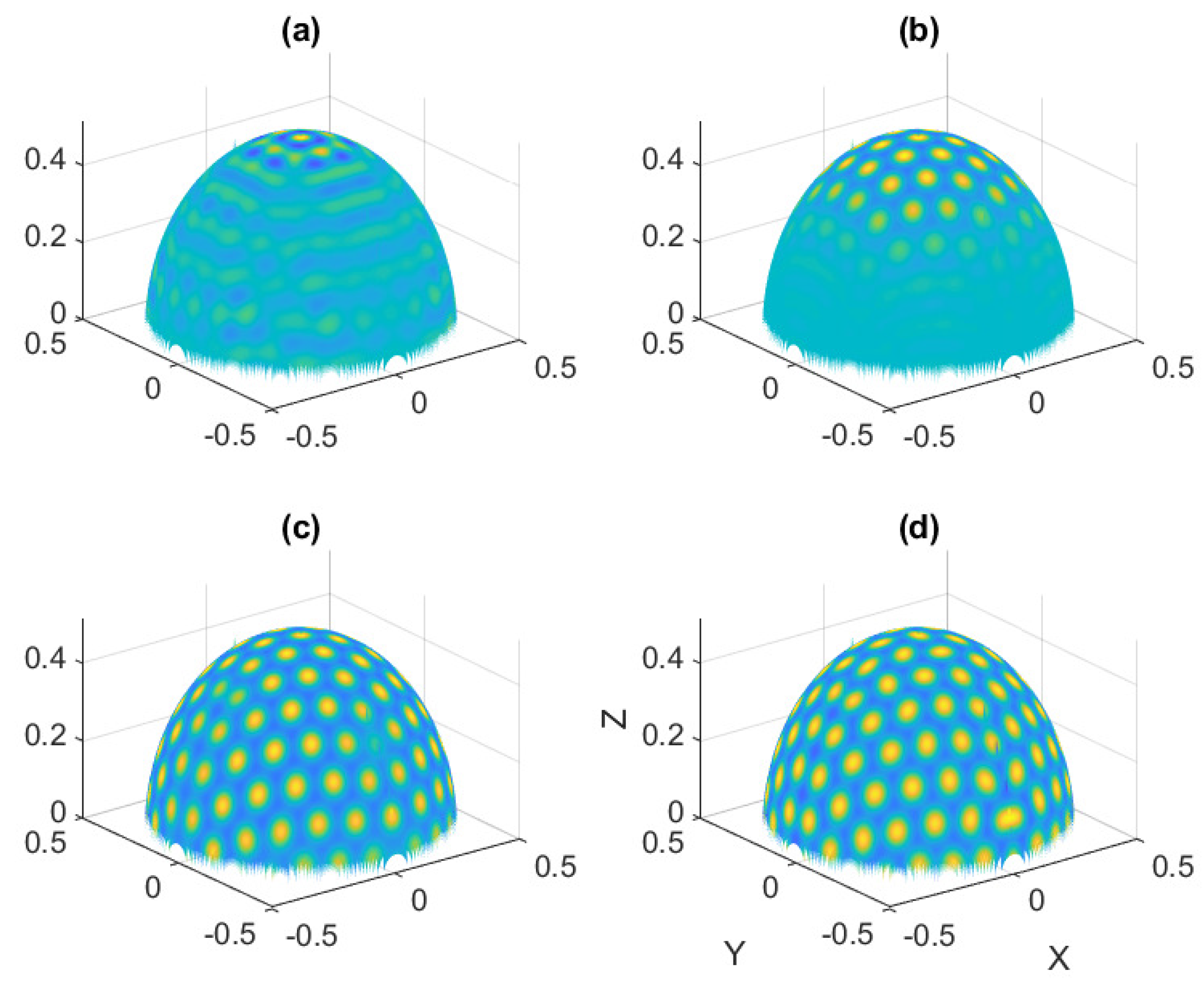

Table 1.
Number of Newton corrections during 100 steps, according to the accuracy parameter . The full algorithm includes convergence acceleration, step length adaptation and Newton correction(s). Required accuracy . The first line reports the results of ANM only followed by Newton corrections, when necessary.
| Pure Newton | 152 | 87 | 53 |
| Full algorithm | 5 | 2 | 0 |
Table 2.
Convergence acceleration by MMPE: a typical example. The table presents the residual before and after the application of MMPE. Seven starting points are considered. Step 34 with the full algorithm and .
Table 2.
Convergence acceleration by MMPE: a typical example. The table presents the residual before and after the application of MMPE. Seven starting points are considered. Step 34 with the full algorithm and .
| r | 0.7 | 0.8 | 0.9 | 1 | 1.1 | 1.2 | 1.3 |
|---|---|---|---|---|---|---|---|
| before | 1224 | 4925 | 17660 | ||||
| after | 1584 |
Disclaimer/Publisher’s Note: The statements, opinions and data contained in all publications are solely those of the individual author(s) and contributor(s) and not of MDPI and/or the editor(s). MDPI and/or the editor(s) disclaim responsibility for any injury to people or property resulting from any ideas, methods, instructions or products referred to in the content. |
© 2025 by the authors. Licensee MDPI, Basel, Switzerland. This article is an open access article distributed under the terms and conditions of the Creative Commons Attribution (CC BY) license (http://creativecommons.org/licenses/by/4.0/).
Copyright: This open access article is published under a Creative Commons CC BY 4.0 license, which permit the free download, distribution, and reuse, provided that the author and preprint are cited in any reuse.


