Submitted:
01 July 2025
Posted:
02 July 2025
You are already at the latest version
Abstract
Understanding psychological change requires a quantitative framework capable of capturing the complex and dynamic relationships among personal constructs. Personal Construct Psychology emphasizes the hierarchical reorganization of bipolar constructs, yet existing qualitative methods inadequately model the reciprocal and graded influences involved in such change. This paper introduces the Presence–Hierarchy (PH) space, a centrality measure for constructs represented within Fuzzy Cognitive Maps (FCMs). FCMs model cognitive systems as directed, weighted graphs, allowing for nuanced analysis of construct interactions. The PH space operationalizes two orthogonal dimensions: Presence, representing the overall connectivity and activation of a construct, and Hierarchy, quantifying the directional asymmetry between influences exerted and received. By formalizing Hinkle’s hierarchical theory within a rigorous mathematical framework, the PH space enables precise identification of constructs that drive or resist transformation. This dual-dimensional model provides a structured method for analyzing personal construct systems, supporting both theoretical exploration and clinically relevant interpretations in the study of psychological change.
Keywords:
Fuzzy Cognitive Maps (FCMs)
; graph theory
; centrality measures
; psychological change
; personal construct psychology
1. Introduction
1.1. Psychological Change and Personal Construct Systems
Grasping psychological change requires a detailed understanding of the complex interplay of meanings individuals construct to interpret and anticipate their experiences. Personal Construct Psychology (PCP) [1] conceptualises this as an evolving system of bipolar constructs that mediate personal anticipation and interpretation of events. Kelly’s foundational model suggests psychological change as a systematic reorganisation of these personal construct systems, involving the adaptation of existing constructs or the introduction of novel ones [2,3].
While Kelly’s model provides a rich qualitative description, it lacks explicit quantification of reciprocal and dynamic influences among constructs. Hinkle [4] sought to address this gap by introducing the laddering technique, emphasizing hierarchical structures among constructs and proposing that constructs higher in this hierarchy (supraordinate constructs) exercise greater influence and display more resistance to change compared to subordinate constructs. However, the inherently qualitative and unidirectional assumptions of laddering limit its capacity to represent the complex, reciprocal, and graded relationships characteristic of actual cognitive systems [5,6].
1.2. Fuzzy Cognitive Maps as Quantitative Models
To systematically represent these intricate relational patterns, Kosko [7] introduced Fuzzy Cognitive Maps (FCMs), a graph-theoretical framework where constructs are represented as nodes interconnected by directed, weighted edges reflecting perceived influences [7,8]. FCMs capture feedback loops, mutual influences, and graded relationships, offering a dynamic model of human cognition that aligns closely with PCP’s anticipatory nature [9,10].
Clinical applications of FCMs, such as through structured elicitation methods like the Weighted Implication Grid (WimpGrid) [11], significantly enhance practitioners’ ability to map cognitive and affective networks with precision. Such mappings reveal critical constructs that guide or resist psychological transformation, offering clinicians robust analytical tools to foster therapeutic insight and intervention [12].
1.3. Centrality Measures in Graph Theory
Despite these advances, quantitatively identifying critical nodes—constructs that significantly shape psychological transformation—remains challenging. Traditional centrality measures in network analysis, initially developed for social networks [13,14,15,16], have been adapted to characterize influential elements within complex psychological networks. However, the directional and weighted nature of FCMs necessitates refined analytical strategies to accurately capture construct influence. Measures such as in-degree, out-degree, and eigenvector centralities have been proposed and adapted specifically for directed and weighted contexts, enhancing the sensitivity of analyses to the nuanced cognitive dynamics underpinning psychological change [10,17].
To address these analytical needs explicitly, this study introduces the Presence-Hierarchy (PH) space, a geometrically grounded analytic framework specifically tailored for interpreting construct centrality within FCMs. The PH space operationalises two critical dimensions: presence, which quantifies the general connectivity and influence activity of a construct, and hierarchy, capturing the directional balance between influences exerted and received. By mathematically formalising the hierarchical differentiation originally proposed by Hinkle, the PH framework significantly advances the capacity to quantitatively analyse construct interrelations within personal meaning systems.
Employing the PH framework within FCMs allows researchers and practitioners to simultaneously identify constructs by their general network prominence (presence) and their hierarchical role within the cognitive system. This dual-dimensional perspective not only offers deeper insight into the mechanisms that drive psychological change, but also facilitates targeted and effective therapeutic strategies. Consequently, the integration of PCP, Hinkle’s hierarchical insights, FCM, and the new PH framework presented here enriches both theoretical understanding and practical intervention methodologies, representing a significant advancement in the mathematical modelling of psychological transformation.
2. Mathematical Foundations
To analyse psychological change, it is essential to establish a formal mathematical framework that captures the relational structure of personal constructs and their dynamic implications. The following foundations define a graph-theoretic model of psychological meaning making, based on the representation of constructs as vectors in bounded spaces, the simulation of hypothetical transformations, and the computation of influence weights between constructs. This section explains how self-perception, ideal goals, and construct interactions can be encoded as algebraic objects and how these structures enable the construction of an FCM that reflects the individual’s psychological topology. The psychological data required to instantiate this model are obtained through the WimpGrid interview protocol [11], a structured assessment methodology to generate personal construct systems. These mathematical definitions provide the basis for deriving a directed graph of meaning relations and for quantifying the centrality and hierarchical role of each construct in psychological change.
2.1. FCM of Psychological Change
To formalise the representation of psychological change, we begin by defining the algebraic objects that capture the structure of an individual’s personal construct system. These objects serve as the foundation for constructing a FCM, where constructs are modeled as nodes, and perceived causal influences among them are represented as weighted directed edges. This mathematical framework enables the translation of qualitative self-perception and ideal self-evaluation, as elicited through the WimpGrid interview [11], into a structured and analyzable model. In what follows, we introduce the definitions and axioms necessary to construct such a map, starting from the self and ideal-self vectors and culminating in a weight matrix that encodes the system of cognitive implications.
Definition 1.
The Self-Now of the individual can be represented as a vector , where n is the number of constructs elicited in the WimpGrid interview, and each component corresponds to the individual’s Self-Now score on construct i within their personal construct system.
Remark 1.
The notation represents the n-dimensional space where each coordinate corresponds to a construct elicited. Each score is bounded within the interval , ensuring a normalized representation of personal meanings. A value of indicates complete alignment with the left pole of the construct, while a value of 1 represents complete alignment with the right pole. Intermediate values correspond to positions between the two poles of the construct, reflecting varying degrees of association.
Definition 2.
The Ideal-Self of the individual can be defined as a vector , where n is the number of constructs elicited in the WimpGrid interview, and each component corresponds to the individual’s Ideal Self score on construct i within their personal construct system.
Definition 3.
The intensities of the hypothetical situations proposed during the interview can be represented as a vector , where n is the number of constructs elicited in the WimpGrid interview, and each component represents the intensity score assigned to a hypothetical situation associated with construct i.
Remark 2.
Following the WimpGrid protocol [11], is computed based on the Self-Now vector and the Ideal-Self vector . Specifically, each is determined as:
Definition 4.
The hypothetical states of the individual (referred to as Hypothetical-Selves) can be represented using a matrix , where each entry represents the hypothetical score assigned to construct i under the influence of hypothetical situation j.
Remark 3.
The diagonal entries are arbitrarily defined as the components of the Self-Now vector for the purposes of subsequent mathematical computations.
Axiom 1
(Linearity of Change). It is assumed that there exists a linear relationship between the proposed change in the hypothetical situation, , and the declared change in the construct j as a result of the influence of the construct i, denoted by . Specifically, this relationship is expressed as:
Remark 4.
The linearity assumption encapsulated in Equation (2) implies that the influence of construct i on construct j can be fully captured through a single proportionality coefficient, . This assumption simplifies the system’s complexity by reducing non-linear dynamics to a manageable linear framework, making it amenable to graph-theoretic and algebraic analysis.
Theorem 1.
Given the current state vector , the hypothetical intensity vector , and the matrix of Hypothetical-Selves M, a weight matrix can be computed. Each entry in W quantifies the sensitivity of construct j to changes in construct i and is defined as:
Proof.
To compute the weight matrix W, consider the following reasoning:
- The matrix M encodes the hypothetical selves, where represents the hypothetical score of construct j when construct i undergoes a hypothetical shift (). Thus, reflects how construct j is influenced by changes in construct i.
- The Self-Now vector provides the baseline values for each construct, where is the score for construct j in its present state. The difference therefore measures the deviation of construct j under the hypothetical shift, , associated with construct i from its baseline state.
- The hypothetical intensity vector captures the proposed changes in the interview. The difference quantifies the magnitude of the hypothetical change introduced to construct i.
- From the Linearity of Change Axiom (Axiom 1), we assume that the relationship between the change in construct i and the corresponding change in construct j can be described as proportional. This proportionality is expressed by:where is the proportionality coefficient that quantifies the influence of construct i on construct j.
- Applying this axiom to the hypothetical scenario, we relate the deviation of construct j () to the magnitude of the shift introduced to construct i (). Specifically, the weight is given by normalizing the deviation with respect to the hypothetical intensity :
- Equation (3) quantifies the sensitivity of construct j to changes in construct i under the assumption of linearity. This process is applied to all pairs of constructs , resulting in the weight matrix W, which captures the pairwise relationships across the entire system.
□
Example 1.
Given the score matrix in Figure 1, we can operationalize it as follows: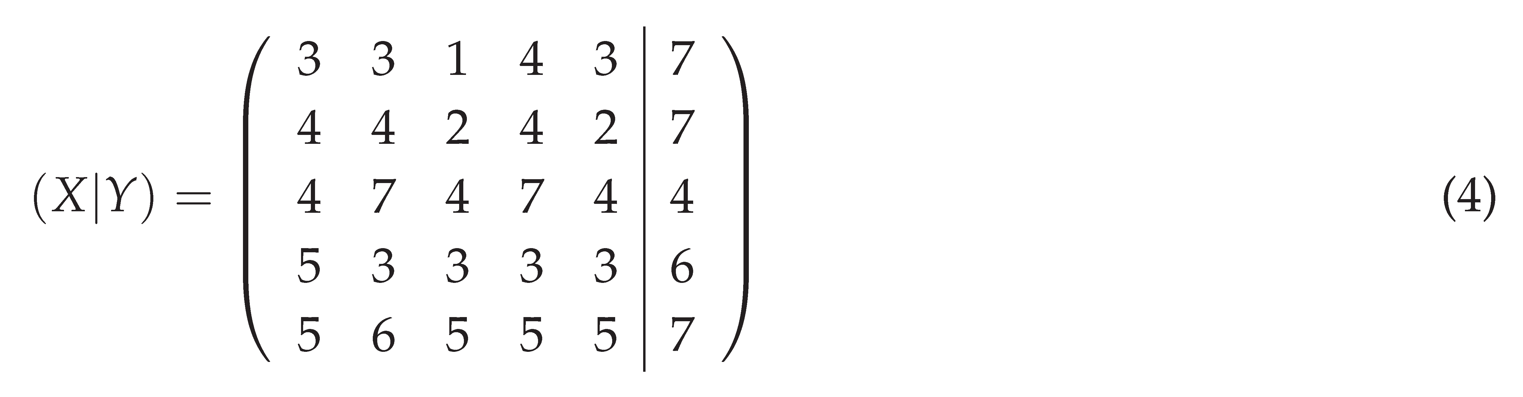
Applying a rescaling transformation from the interval to , we obtain a normalized matrix: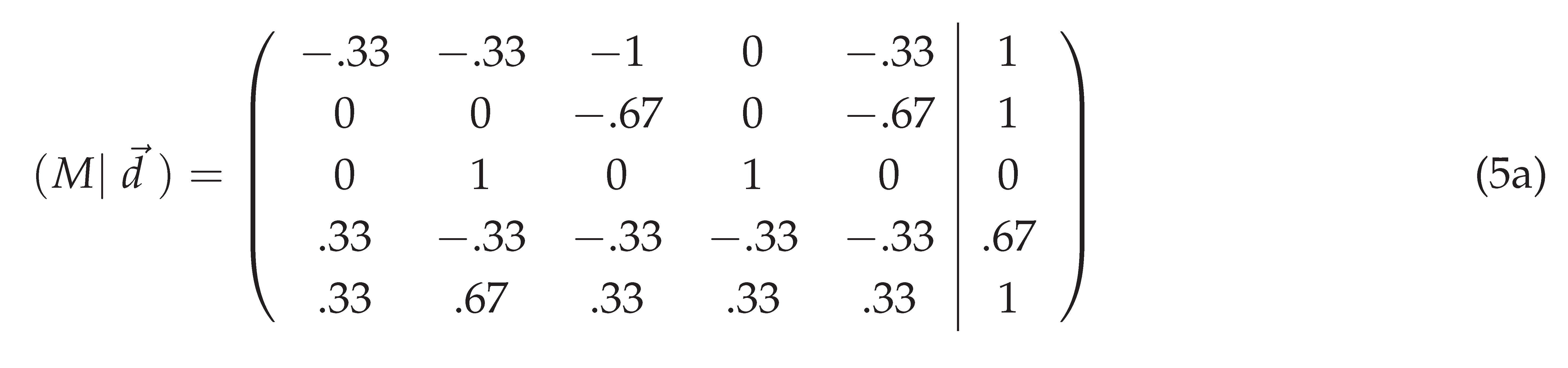
Using the normalized matrix and applying Weight Matrix Calculation Theorem (1), we can calculate the self vector , the ideal vector , and the weight matrix W for the example:
Definition 5.
Given a weight matrix , a self vector , and an ideal vector , there exists a directed graph such that:
- , where each vertex corresponds to a construct.
- , where if and only if .
- assigns attributes to vertices, where .
- assigns weights to edges, where .
Figure 2 illustrates the directed graph G constructed from the data presented in Example 1, displaying both the edge weights and the node attributes associated with each construct.
The resulting graph G provides a visual and mathematical representation of the relationships between constructs. The directed edges encode the influences derived from W, while the node attributes enrich the graph with the self and ideal scores, allowing for a comprehensive analysis of both structural relationships and individual goals.
2.2. PH Space
Definition 6.
Let be a vertex of the graph G, and let denote the weights associated with the edges of G. We define two measures for the vertex : the in-degree and the out-degree , as follows:
Remark 5.
The in-degree and out-degree measures defined above are adapted from the graph-theoretic approach presented by Borgatti [18].
Axiom 2
(Vertex Hierarchy). Let be a vertex in the graph G. The hierarchical state of is determined by the relationship between its in-degree and out-degree , and is defined as follows:
- is said to be supraordinate if , meaning the vertex exerts more influence (outputs) than it receives (inputs).
- is said to be subordinate if , meaning the vertex is more influenced by other vertices (inputs) than it influences them (outputs).
- is said to be neutral if , meaning the vertex has an equal balance of influence received (inputs) and exerted (outputs).
Remark 6.
The concept of hierarchy described here is inspired by the framework introduced by Hinkle [4], who suggested that constructs that exert greater influence on a system while being less influenced themselves are considered to be more supraordinate. This principle extends naturally to vertices in a graph, where the relationship between inputs and outputs reflects their hierarchical role within the structure.
Theorem 2.
Let be a directed graph, where each vertex has an in-degree and an out-degree , to compute presence and hierarchy , we apply the following linear transformation to :
Remark 7.
The Presence index quantifies the total connectivity of vertex , combining its in-degree () and out-degree (). And Hierarchy index quantifies the net difference between the in-degree and out-degree of vertex .
Proof.
Let represent the in-degree and out-degree of a vertex in a directed graph . The goal is to compute two indices, Presence index () and Hierarchy index (), by transforming the original vector into a new coordinate system. The transformation is defined by the matrix:
This matrix corresponds to a rotation of the original coordinate system by counterclockwise, scaled by . Applying this transformation to the vector , we compute the Equation (8):
Performing the matrix multiplication, we obtain:
Factoring out , these simplify to:
Geometrically:
- Presence index () represents the projection of the vector onto the axis defined by , capturing the total connectivity of vertex , i.e., .
- Hierarchy index () represents the projection of the vector onto the axis defined by , capturing the net difference between and , i.e., .
Thus, the transformation rotates the space by so that the new axes correspond to the desired components of Presence () and Hierarchy (). The scaling factor ensures that the magnitudes of the transformed indices are appropriately normalized. □
The PH space visualization (Figure 3) thus provides a concise and interpretable summary of the relational dynamics within personal construct systems. By clearly distinguishing constructs according to their centrality and hierarchical roles, this geometric framework not only facilitates theoretical understanding but also supports targeted clinical interventions. Clinicians can readily identify influential constructs that serve as critical leverage points for therapeutic change, enabling a systematic and strategically informed approach to psychological intervention.
2.3. Properties of the PH Space
This section presents a formal characterization of the PH space. The analysis is organized into two parts. First, we demonstrate that the PH space satisfies the defining properties of a two-dimensional convex cone in . Second, we examine the projection as a limiting representation of all possible weighted directed graphs of increasing order n, assuming continuous-valued edge weights in the range .
2.3.1. Bounding Theorem and Geometric Constraint
Theorem 3.
All points resulting from this transformation satisfy the following constraint:
Proof.
Non-negativity of P. Since , it follows that:
Bounding inequality .
Boundary cases. Equality holds in the following cases:
- If , i.e., the node is a pure source, then .
- If , i.e., the node is a pure sink, then . □
2.3.2. Geometric Formulation
Any point in the PH space results from a linear transformation applied to the normalized counts of in-degree and out-degree connections of a construct in an FCM. As shown above, each point satisfies:
This inequality defines a conic region in , with vertex at the origin and bounded by the rays and . At , hierarchy necessarily vanishes, yielding the origin. As P increases, the admissible range of H expands symmetrically.
Definition 7.
The PH space is defined as the set:
This constraint arises naturally from the linear transformation applied to node in-strength and out-strength in a weighted directed graph. Since both quantities are defined as non-negative sums of edge weights, it follows that and for all projected nodes. Therefore, the image of any fuzzy cognitive map under the PH transformation lies within C.
Theorem 4
(Convex Cone Structure). The set C defined in Definition 7 satisfies the axioms of a convex cone.
Proof.
We prove that C satisfies the three fundamental properties:
1. Closure under non-negative scalar multiplication. Let and . Then:
Figure 4 illustrates this property: scaling a vector in preserves cone membership.
2. Closure under vector addition. Let . Then:
Figure 5 exemplifies vector addition within .
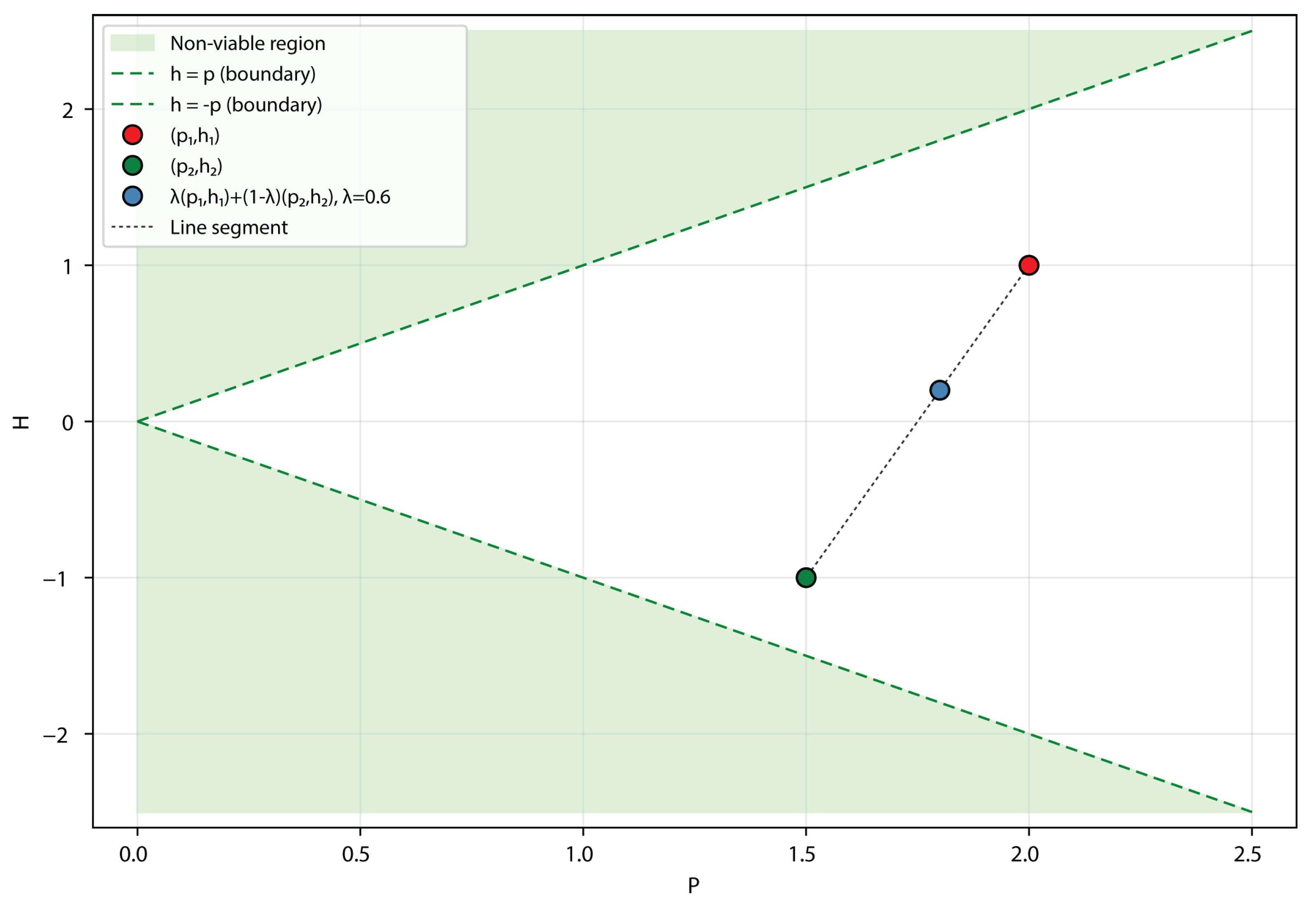
3. Closure under convex combinations. Let and define:
Then:
□
Figure 6 exemplifies convex combinations in .
2.3.3. Graph Projections and Asymptotic Behavior
Let denote the set of all possible FCMs of order n, where each directed edge can take any value in . Each node maps to a pair via the transformation described above.
Theorem 5
(Asymptotic Density). For fixed n, the projection of is a compact, continuous, non-convex subset of C. As , the union of projections densely fills C.
Compactness and continuity. Since the projection is a continuous function of the compact set , its image is compact.
Non-convexity. Consider and the points:
- -
- (source: )
- -
- (balanced: )
Both are achievable. Their midpoint requires . However, in any 3-node graph:
- Achieving A requires a node with (max out-strength).
- Achieving C requires another node with (max connections).
This exhausts all edge slots, leaving no capacity for a node with at M. Thus, .
Asymptotic density. Let be the PH space defined by . Then, for any and any , there exists and a fuzzy cognitive map of order n such that the projection of contains a node satisfying .
Proof.
Let and be arbitrary. Define:
By construction, due to . Our goal is to realize node strengths within an additive error that guarantees in PH space.
Let and be arbitrary. Define
Then, if we construct a node with approximate in-strength and out-strength satisfying
it follows by linearity of the PH transformation that
To achieve such an approximation, note that any desired value of can be represented as the sum of outgoing connections with weight 1, plus a residual outgoing edge with weight , provided this residual exceeds . The same construction applies symmetrically for by selecting incoming edges in an analogous manner.
Define
and choose
This choice of n ensures that there are enough nodes to provide the required number of incoming and outgoing connections without violating the no self-loop constraint inherent to the graph definition.
To complete the construction, assign all other edge weights in to values strictly less than . This guarantees that their cumulative contribution to the in-strength or out-strength of the approximating node remains below and does not affect the targeted precision.
Thus, we have constructed a graph containing a node with approximate strengths within of , and consequently, a projection within of in the PH space. Since and were arbitrary, the density of projections in C follows as .
Hence, its projection lies within distance of in the PH space. Since and were arbitrary, the union of projections over increasing n is dense in C.
□
2.3.4. Interpretational Implications
The PH space offers a faithful embedding of the topology and influence patterns of FCMs. Although it does not capture semantic distances to ideal constructs, it provides a scalable and rigorous geometric framework for examining the overall graph architecture.
In summary, the PH space is defined by the constraint , forming a bidimensional convex cone in . This structure supports both the geometric interpretation of construct systems and their formal modeling as the number of nodes n increases, approaching a dense representation in the limit.
3. Discussion
3.1. Applications
The PH space, defined as a bidimensional convex and self-dual cone, admits several analytically grounded applications within the modeling of personal construct systems.
(a) Identification of hub constructs. Constructs located in the high-P region and exhibiting high Mahalanobis distance from the centroid can be interpreted as structural hubs within the cognitive system. To ensure interpretive validity, the analysis is restricted to constructs with , and Mahalanobis distance is computed relative to the empirical covariance structure of this subset. Constructs exceeding a predefined threshold (e.g., percentile) are identified as hubs, reflecting both prominence and deviation from the system’s central configuration.
(b) Dynamic trajectories and attractors. The convex geometry of the PH space allows for the analysis of simulated activation dynamics derived from fuzzy cognitive maps. Trajectories projected within the cone may exhibit convergence toward fixed points or bounded regions, interpretable as cognitive attractor states. These attractors may correspond to stable interpretative configurations, enabling formal study of equilibrium, rigidity, or response to perturbation in personal construct systems.
(c) Test-retest stability assessment. The geometric structure also supports the quantification of temporal stability across repeated assessments. Displacement of constructs in the PH space can be evaluated using Euclidean or Mahalanobis distances, allowing researchers to distinguish between stable core constructs and volatile peripheral ones. This approach provides an idiographic measure of consistency, sensitive to both structural position and system-wide distribution.
Each application benefits from the formal constraints of the PH space, enabling statistically consistent and geometrically interpretable operations within a reduced-dimensional framework.
3.2. Limitations and Future Research Directions
(a) Dimensionality reduction. The projection onto the PH plane reduces a potentially high-dimensional system of construct interrelations to two summary dimensions. While this facilitates visualization and analysis, it also entails a loss of information. Further investigation is required to assess which properties of the original system are preserved or distorted by the transformation, and whether the PH space can be extended to higher-dimensional analogues.
(b) Lack of evaluative distance representation. The PH projection reflects the structural connectivity of constructs within a fuzzy cognitive map, encoding their total influence (Presence) and directional balance (Hierarchy). However, it does not represent the evaluative proximity or distance of constructs relative to an ideal self or desired pole. This distinction is particularly relevant in clinical or developmental applications where the salience of a construct may depend not only on its centrality, but also on its alignment with aspirational goals. Future research could explore hybrid projections that integrate both structural and evaluative dimensions, or combine the PH space with discrepancy-based metrics.
(c) Empirical validation. Finally, while the PH space has demonstrated utility in exploratory analyses (e.g., identification of hubs or stability assessment), systematic empirical validation is still required. Future research should examine how constructs identified as central or stable in the PH space correspond to external psychological variables such as symptomatology, well-being, or therapeutic outcomes.
Author Contributions
Conceptualization, A.S., C.H., L.A.S. and L.B.; methodology, A.S. and C.H.; software, A.S.; validation, A.S., C.H., L.A.S. and L.B.; formal analysis, A.S. and C.H.; writing—original draft preparation, A.S. and C.H.; writing—review and editing, A.S., C.H., L.A.S. and L.B.; visualization, A.S. and C.H.; supervision, L.A.S. and L.B.; project administration, L.A.S. and L.B. All authors have read and agreed to the published version of the manuscript.
Funding
This research received no external funding.
Acknowledgments
Conflicts of Interest
The authors declare no conflicts of interest.
Abbreviations
The following abbreviations are used in this manuscript:
| FCM | Fuzzy Cognitive Map |
| PCP | Personal Construct Psychology |
| PH | Presence–Hierarchy |
| WimpGrid | Weighted Implication Grid |
References
- Kelly, G.A. The Psychology of Personal Constructs; Norton: New York, 1955.
- Fransella, F.; Bell, R.; Bannister, D. A Manual for Repertory Grid Technique; John Wiley & Sons: Chichester, UK, 2004.
- Procter, H.; Winter, D.A. Personal and Relational Construct Psychotherapy; Palgrave Macmillan: London, 2020.
- Hinkle, D.N. The Change of Personal Constructs from the Viewpoint of a Theory of Construct Implications. PhD thesis, Ohio State University, Columbus, OH, 1965.
- Bell, R.C. Did Hinkle prove laddered constructs are superordinate? A re-examination of his data suggests not. Personal Construct Theory and Practice 2014, 11, 1–4. [Google Scholar]
- Korenini, B. What do Hinkle’s data really say about laddering? Personal Construct Theory and Practice 2016, 13. [Google Scholar]
- Kosko, B. Fuzzy cognitive maps. International Journal of Man-Machine Studies 1986, 24, 65–75. [Google Scholar] [CrossRef]
- Wang, L.X.; Mendel, J.M. Generating fuzzy rules by learning from examples. IEEE Transactions on Systems, Man, and Cybernetics 1992, 22, 1414–1427. [Google Scholar] [CrossRef]
- Tsadiras, A.K. Fuzzy cognitive maps for decision support in social systems. Journal of Systems Research and Behavioral Science 2008, 25, 285–293. [Google Scholar]
- Felix, G.; Nápoles, G.; Falcon, R.; Vanhoof, K. A review on methods and software for fuzzy cognitive maps. Artificial Intelligence Review 2019, 52, 1707–1737. [Google Scholar] [CrossRef]
- Sanfeliciano, A.; Sául, L.A.; Botella, L. Weighted implication grid: A graph-theoretic approach to modelling psychological change. Frontiers in Psychology 2025. In press.
- Sanfeliciano, A.; Saúl, L.A. WimpTools: A Graph-Theoretical R Toolbox for Modeling Psychological Change (1.0.0), 2025. [CrossRef]
- Freeman, L.C. Centrality in social networks conceptual clarification. Social Networks 1978, 1, 215–239. [Google Scholar] [CrossRef]
- Sabidussi, G. The centrality index of a graph. Psychometrika 1966, 31, 581–603. [Google Scholar] [CrossRef] [PubMed]
- Freeman, L.C. A set of measures of centrality based on betweenness. Sociometry 1977, 40, 35–41. [Google Scholar] [CrossRef]
- Bonacich, P. Power and centrality: A family of measures. American Journal of Sociology 1987, 92, 1170–1182. [Google Scholar] [CrossRef]
- Özesmi, U.; Özesmi, S.L. Ecological models based on people’s knowledge: a multi-step fuzzy cognitive mapping approach. Ecological Modelling 2004, 176, 43–64. [Google Scholar] [CrossRef]
- Borgatti, S.P. Centrality and network flow. Social Networks 2005, 27, 55–71. [Google Scholar] [CrossRef]
Figure 1.
WimpGrid Score Matrix (Scale 1–7), used to elicit and structure the individual’s personal construct system. Each row corresponds to a bipolar construct (e.g., Anxious–Calm), and each column represents a hypothetical self-state: the first five columns depict imagined selves resulting from targeted changes in each construct, while the sixth column represents the Ideal-Self. Cells are filled with self-assigned ratings from 1 to 7, where 1 denotes complete alignment with the left pole and 7 with the right pole. Blue cells indicate the participant’s current Self-Now scores; green cells indicate their Ideal-Self scores; yellow cells highlight constructs where the participant anticipates significant change if another construct is modified.
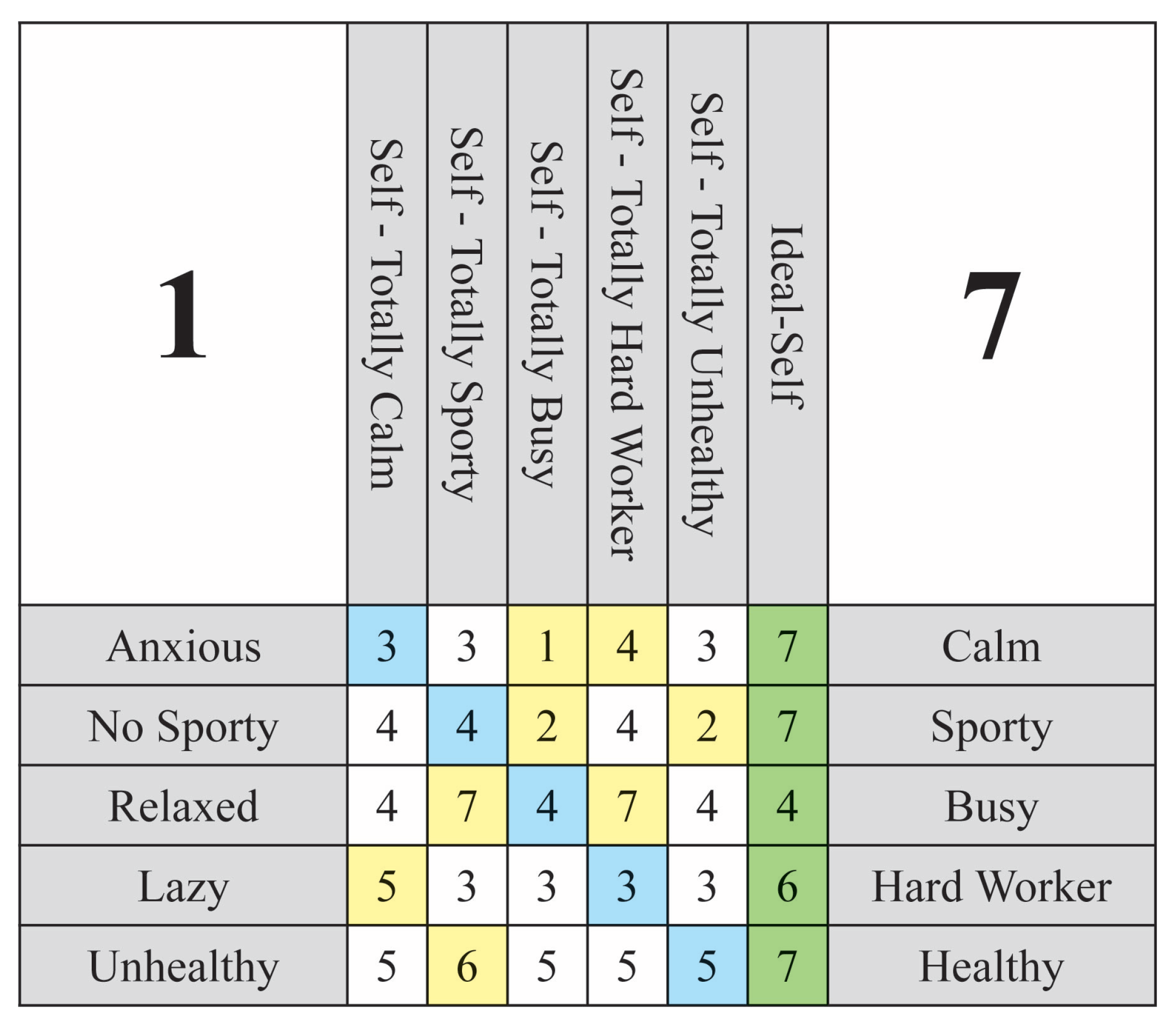
Figure 2.
Directed graph representation of the personal construct system derived from the weight matrix W in Example 1. Each node corresponds to a bipolar construct, positioned and styled according to its psychological attributes. Node color encodes congruence with the Ideal-Self: green indicates full congruence (), red indicates discrepancy (), yellow marks undefined ideal values (), and grey indicates undefined self-perception (). Node size reflects the absolute self-score , representing the construct’s salience in current self-identity. Directed edges represent cognitive implications with black denoting a direct relationship () and red an inverse relationship (). Edge thickness encodes the absolute weight , reflecting the strength of influence. This graph provides an interpretable structural summary of the FCM, supporting both visual intuition and algebraic analysis of psychological change dynamics.Graph generated using WimpTools [12].
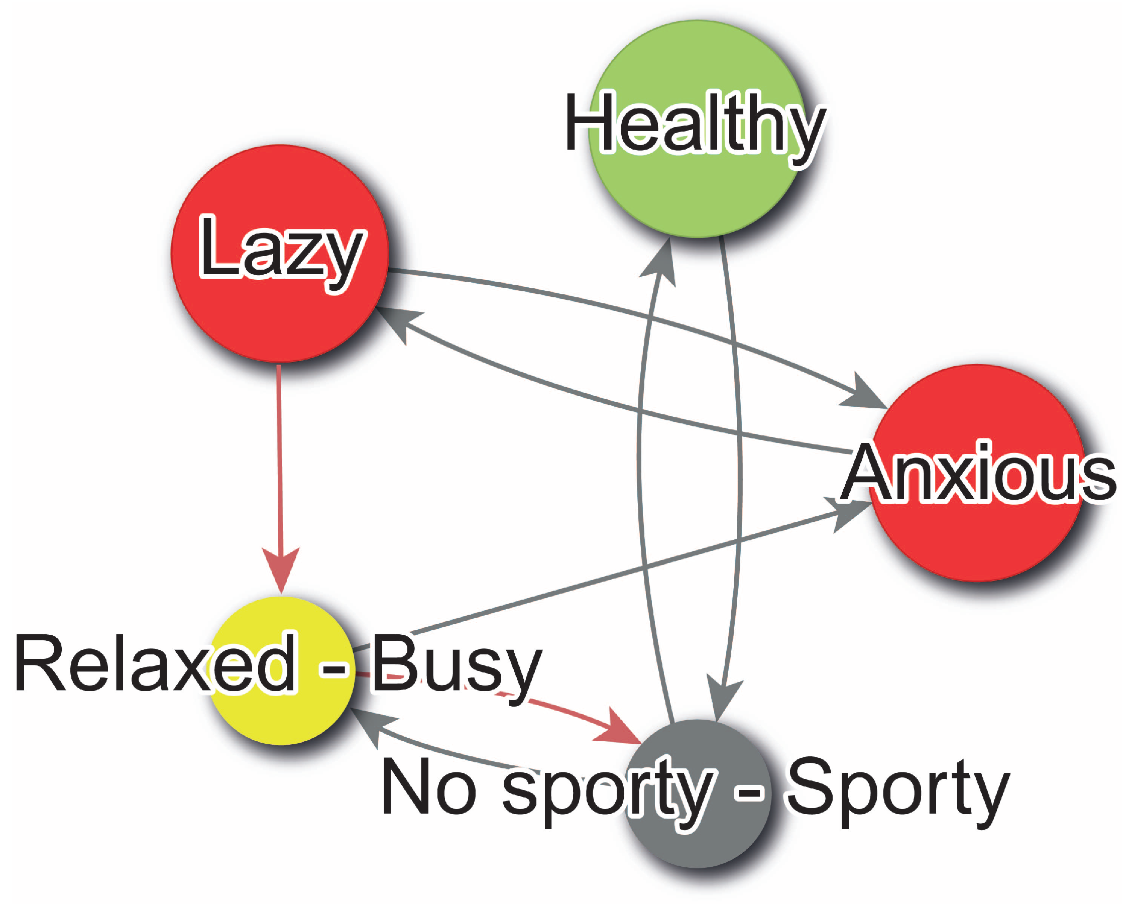
Figure 3.
PH space representation of the psychological constructs from Example 1. Each construct is positioned according to its presence (overall connectivity) and hierarchy (directional balance of influence). Constructs toward the upper region (positive hierarchy) indicate supraordinate roles, exerting greater influence, while constructs in the lower region (negative hierarchy) indicate subordinate roles, being more influenced by others. Proximity to the right side signifies higher overall centrality and connectivity within the cognitive network.
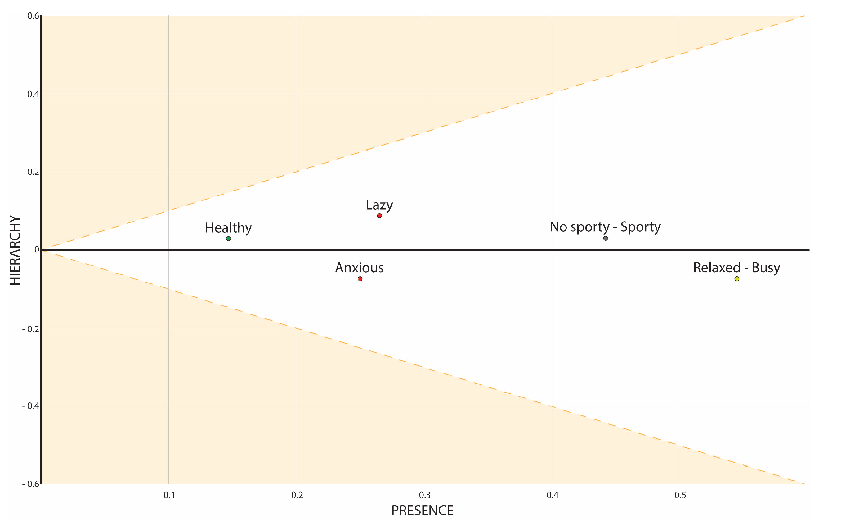
Figure 4.
Closure under scalar multiplication (Theorem 4, Property 1)
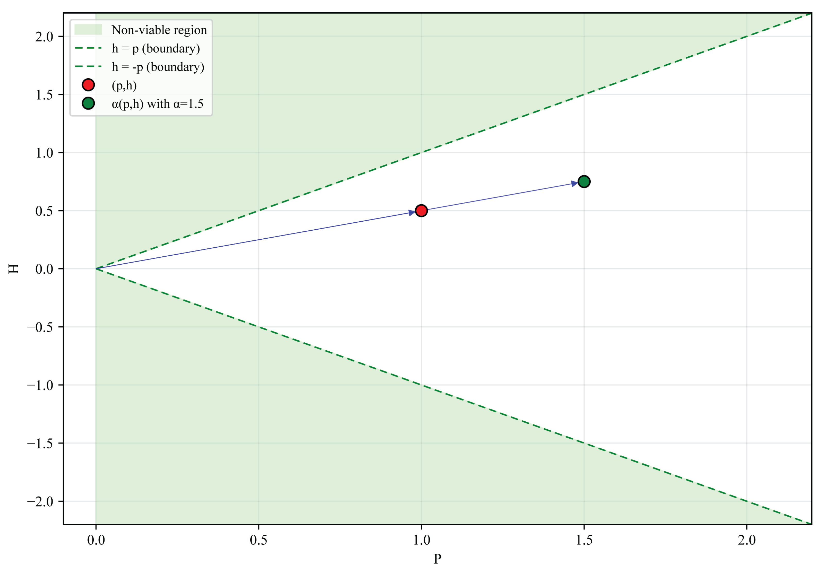
Figure 5.
Exemplification of vector addition (Theorem 4, Property 2)
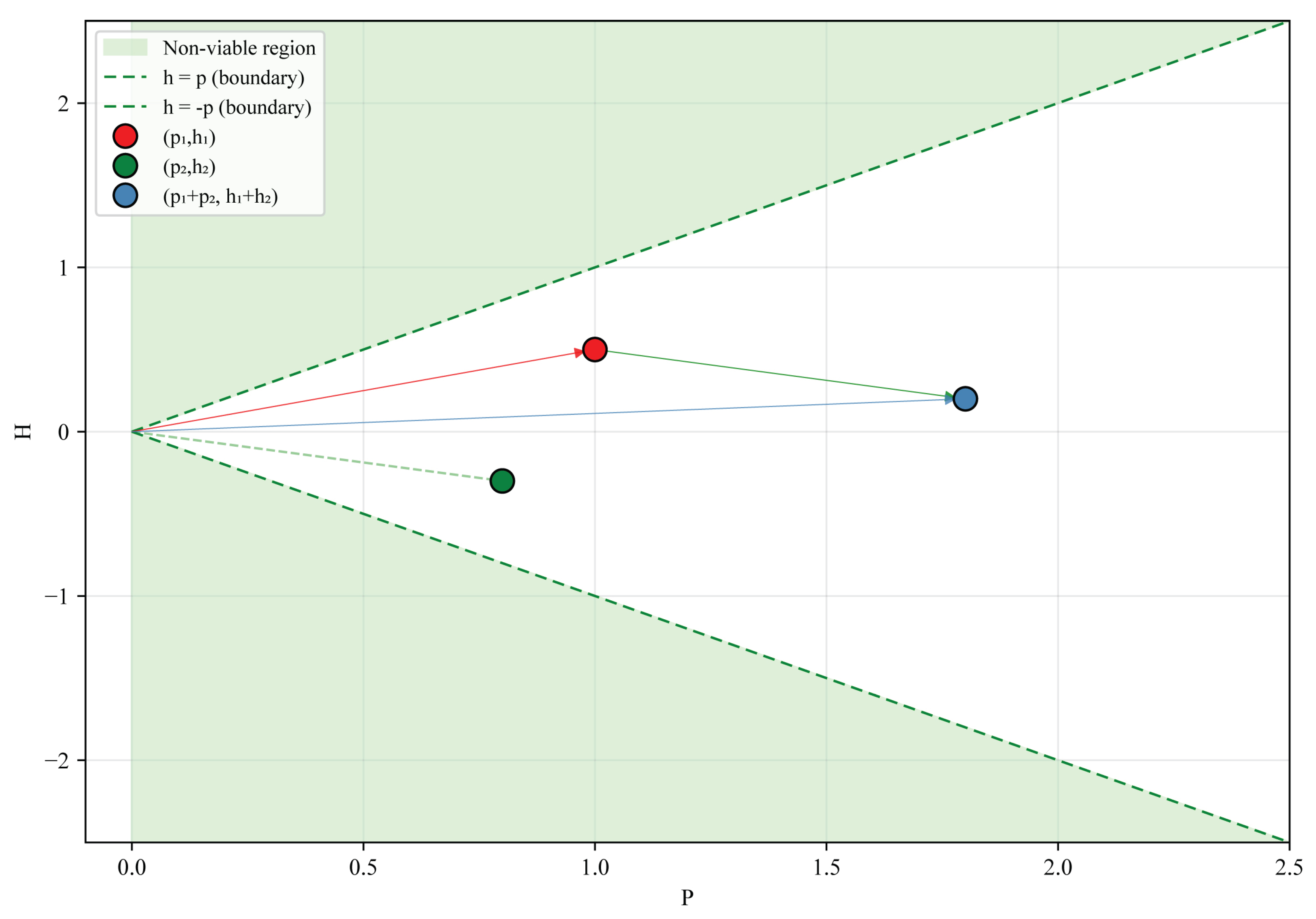
Figure 6.
Convex combinations (Theorem 4, Property 3)
Disclaimer/Publisher’s Note: The statements, opinions and data contained in all publications are solely those of the individual author(s) and contributor(s) and not of MDPI and/or the editor(s). MDPI and/or the editor(s) disclaim responsibility for any injury to people or property resulting from any ideas, methods, instructions or products referred to in the content. |
© 2025 by the authors. Licensee MDPI, Basel, Switzerland. This article is an open access article distributed under the terms and conditions of the Creative Commons Attribution (CC BY) license (http://creativecommons.org/licenses/by/4.0/).
Copyright: This open access article is published under a Creative Commons CC BY 4.0 license, which permit the free download, distribution, and reuse, provided that the author and preprint are cited in any reuse.


