
Submitted:
30 June 2025
Posted:
02 July 2025
You are already at the latest version
Abstract
In many research fields, it is quite common to deal with multiple data sets containing information about the same group of individuals, where one data set aims to explain the others. To address this need, a new multiway regression method called Binary 3-way PARAFAC Partial Least Squares (Bin-3-Way-PARAFAC-PLS) is introduced. This method is specifically designed for the case where a three-way real-valued data array serves as the explanatory role, together with a matrix of binary response data. An algorithm implementing this method is provided, along with its practical application. Additionally, biplot representations are described to assist in the interpretation of the results. The software necessary to implement the method is also provided. Finally, the proposed method is applied to a data set from psychology to demonstrate its usefulness in addressing real-world problems.
Keywords:
binary
; N-PLS
; multilinear PLS
; PARAFAC
; biplot
1. Introduction
The prediction of a dependent variable (y) based on a set of multidimensional independent variables (x) has attracted significant interest across various fields. A commonly used approach for this prediction is Partial Least Squares (PLS) [1,2], which was originally developed for continuous data. PLS identifies a set of linear combinations of the predictor variables that exhibit the highest correlation with the response variables.
Multiway data, also known as higher-order data or tensors, has become increasingly common in various areas of our information society, such as bioinformatics [3], chemometrics [4], neuropsychology [5] and personality research [6]. In the context of multiway data, a ’way’ represents one of the dimensions along which the data is structured. For example, in a dataset with three dimensions, these might be subjects, variables and occasions. The term ’mode’ is used to specify the type of entity associated with each dimension. Typically, the number of ways and modes are equal, as in a three-dimensional dataset where each way corresponds to a different entity type (e.g. subjects, variables and occasions). However, there are scenarios where the number of modes is less than the number of ways. An example is a two-mode, three-way dataset where one entity type occurs in more than one dimension. This occurs, for example, when objects are compared across multiple subjects, resulting in a data structure where the same objects are repeated across dimensions [7,8]. To analyze these types of data, traditional methods based on Principal Component Analysis (PCA) [9] have been extended to accommodate the complexity of higher-dimensional structures. Techniques such as Tucker decomposition [10,11,12] and PARAFAC decomposition [13,14,15] are among the most widely used. Tucker decomposition generalizes PCA by decomposing the data into a core tensor and factor matrices, with each factor matrix corresponding to one of the modes of the tensor [16]. On the other hand, PARAFAC decomposes the tensor into a sum of component tensors, where each component is a rank-1 tensor.
Given the prevalence of this type of data, Partial Least Squares (PLS) has been extended to accommodate such data structures, facilitating the prediction of from , where and/or are three-way data arrays. Specifically, [17] first combined the PARAFAC three-way analysis method with the PLS method. This method, called multilinear PLS (N-PLS), is thus a mixture of a trilinear model (PARAFAC) and PLS [18]. Subsequently, [19] propose a modification of the above model that aims not to improve the prediction of the dependent variables, but rather to improve the modeling of the independent variables. To achieve this, they rely on the distinction between low-rank and subspace approximation inherent in the PARAFAC and Tucker3 models. More recently, Sparse N-Way Partial Least Squares with L1 penalization has been proposed [20,21], which aims to achieve lower prediction errors by filtering out variable noise, while improving the interpretability and utilization of the N-PLS method.
The methods discussed earlier are designed for scenarios where both predictors and responses are continuous. When the response matrix contains binary variables, Partial Least Squares Discriminant Analysis (PLS-DA) [22] is often employed, which essentially fits a PLS regression to a dummy or fictitious variable. [23] introduced a PLS model for a single binary response, analogous to the PLS-1 model. [24] proposed the PLS-BLR method, a Partial Least Squares method for situations where the responses are binary and the predictors are continuous. Subsequently, they extended this approach to address cases where both the predictors and the responses are binary [25], introducing additional adaptations to handle this more complex scenario. This method, known as Binary Partial Least Squares Regression (BPLSR), further broadens the applicability of Partial Least Squares methods in analyzing binary data structures. This approaches extend PLS generalized linear regression [23] from a single response variable (PLS1) to multiple responses (PLS2), introducing dimension reduction, a feature not present in the original method. In the context of genomic data, other studies [26,27] applied Iteratively Re-weighted Least Squares (IRWLS) to handle binary responses with numerical predictors.
This paper proposes an extension of the N-PLS method to deal with scenarios where there is a set of binary dependent variables alongside a three-way data set of explanatory variables. It is therefore a combination of the previously mentioned N-PLS and PLS-BLR methods. Although the proposed BIN-3-Way-PARAFAC-PLS method is currently designed and tested for three-way data arrays, the underlying principles and techniques hold the potential for extension to N-way configurations. This limitation to three-way data is explicitly addressed throughout the manuscript to ensure clarity and accuracy. In addition, the use of biplot methods is proposed to graphically assess prediction quality and to identify explanatory variables that are more strongly associated with response variables. The biplot used will be a combination of logistic biplot [28,29] and interactive biplot [30].
The paper is structured as follows: Section 2 provides a brief overview of the PLS methods, followed by the introduction of the Bin-3-Way-PARAFAC-PLS method in Section 3, which allows PLS analysis of a matrix of binary responses alongside a three-way data array of explanatory variables. An algorithm for calculating model parameters is outlined in this section. Section 4 introduces a biplot method for visual assessment of the results obtained with Bin-3-Way-PARAFAC-PLS. Section 5 illustrates the application of the proposed method, and finally Section 6 offers concluding remarks and outlines potential future research directions.
2. A Brief Overview of PLS Models for Continuous Data
In this work, scalars are denoted by italic lowercase, vectors by bold lowercase, matrices by bold uppercase, and three-way data arrays by underlined bold uppercase. The letters I, J, K, L are used to denote the dimension of different orders. The abbreviations for the different PLS models are Bi/Tri-PLS-1/2/3, where the prefix (Bi/Tri) indicates the order of and the last number (1/2/3) indicates the order of , e.g. Bi-PLS3 refers to PLS with as a data matrix and as an 3-way data array.
Lets begin with a brief overview of bi-PLS1. Let be and column centered (and scaled if necessary) matrices. The bi-PLS1 algorithm consists of two main steps. In the first step for each component, a rank one model of and y is constructed. Then in a second step, these models are subtracted from and , resulting in residuals. From these residuals a new set of components is obtained. It is therefore a question of finding a one-component model of such that where and are the scores and the weights respectively. This is done by maximizing the following function
subject to or equivalently
subject to
It can be verified that the value of the above expression is maximal when
or, in other words, if is the left singular vector of . Once the first component is obtained, and are deflated and the second component is sought following the same process.
Similarly, when is a three-way data array , the goal of the algorithm is to maximize the covariance between and . Let be the unfolded version [31] of , then it is a matter of finding latent spaces and that maximise the covariance between and , so that can be written as:
where is the matrix of scores in the first mode, and are the weights of the second and third mode respectively, ⊙ is the Khatri-Rao product (column-wise Kronecker product) [32], is a matrix of residuals and S is the number of components. The above decomposition corresponds to the PARAFAC model for three-way arrays. In this case the function to be maximized is
where and can be obtained using the singular value decomposition (SVD) of , being the matrix obtained as .
Given the number of components S, the full algorithm for the Tri-PLS1 model is as follows:
| Algorithm 1 Tri-PLS1 for S components |
|
In case where there are several dependent variables , can be expressed as:
where is the matrix of scores, is the loading matrix and is a matrix of residuals.
The model is estimated in such a way that the covariance between and is maximized. The prediction model between and can be expressed as:
where matrix represents the regression coefficients.
The algorithm that implements the Tri-PLS2 model for S components is as follows:
| Algorithm 2:Tri-PLS2 for S components |
|
3. Bin-3-Way-PARAFAC-PLS
The previous linear model is not valid and a logit transformation must be performed if the response matrix is binary. In this case, the expected values of the binary response are probabilities and the logit function is used as the link function. Let be = , then
This equation is a generalization of Equation 2 except now it is needed a vector with intercepts for each variable, given that binary matrix cannot be centered in the same way as continuous matrix. Each probability can be expressed as
The procedure for estimating the parameters of the model is similar to the one described in [24]. The cost function in this case is as follows:
The objective is to estimate the parameters , and that minimize the value of the above cost function. There are no closed-form solutions for the optimization problem; therefore, an iterative approach is employed, where we generate a sequence of progressively smaller values for the loss function with each iteration. The gradient method is applied recursively, solving for one component at a time while keeping the others fixed. The update for each parameter is as follows:
for a choice of .
The corresponding gradients are:
The algorithm will iteratively compute parameters for rows and columns for each dimension s, keeping fixed the parameters obtained for each previous dimension, with the aim of deriving uncorrelated components. Previously, the constants must be determined separately.
In logistic regression, a common issue known as separation can arise when the data are perfectly separable by a linear combination of the predictors. In such cases, the maximum likelihood estimator fails to exist and diverges to infinity [33]. Even in situations of quasi-separation, where the separation is not complete, the maximum likelihood estimator can become highly unstable.
To address this problem, a typical approach is to employ a penalized likelihood method [34]. This technique incorporates a penalty term into the likelihood function, promoting smaller coefficient values and improving stability. In this work, we apply the Ridge penalty [35] to mitigate the effects of separation.
Combining the Tri-PLS2 algorithm with the previously discussed method for obtaining the components of a binary matrix, we would have the following algorithm:
| Algorithm 3: Bin-Tri-PLS2 for S components |
|
The regression coefficients of the response variables on the observed variables can be obtained as follows:
then
with
i.e., are the regression coefficients relative to the observed variables.
4. Bin-3-Way-PARAFAC-PLS Biplot
In this section, a biplot representation is proposed for the graphical visualization of the results obtained by the Bin-3-Way-PARAFAC-PLS algorithm. It begins with a brief review of the biplot for continuous data to introduce the biplot for binary data, known as the logistic biplot. The combination of the PLS-biplot [36] with the logistic biplot [28,29] and the interactive biplot [30] for three-way data will result in the proposed Bin-3-Way-PARAFAC-PLS biplot.
4.1. Classical Biplot
The biplot was originally introduced by [37] and extended by [38] to visualise relationships between variables and observations in a multivariate data set. It has since been widely adopted in fields as diverse as ecology, chemometrics and the social sciences because it provides a comprehensive graphical representation of both observations and variables simultaneously in a low-dimensional space.
It is a well-known fact that any matrix with rank R can be decomposed into two matrices, of size and of size , such that . This decomposition enables the assignment of vectors (row markers) to each of the I rows of and vectors (column markers) to each column of , which provides a representation of using vectors in an R-dimensional space. In the case of matrices with rank two, this representation occurs in a two-dimensional space (plane), but for higher-rank matrices, an approximation in a reduced-dimensional space (either 2 or 3 dimensions) is obtained, such that .
This factorization, usually achieved by Singular Value Decomposition (SVD), allows the representation of the matrix in a space of reduced dimension such that . Geometrically, this means that the projection of a row marker onto the vector representing a variable approximates the value of the individual on that variable and allows the individuals to be ordered by that variable. It is also possible to interpret the angles formed by two variables or the distances between individuals. The angles between variables in a biplot represent the correlations or associations between them. If two variables form a small angle, this indicates a strong positive correlation between them, while a large angle indicates a weaker or negative correlation. The distances between individuals (observations) in a biplot reflect their similarities or dissimilarities based on the values of the variables. Closer distances indicate greater similarity, while further distances indicate greater dissimilarity.
4.2. Logistic Biplot
Let be a binary matrix and , we have that
Apart from the constant vector , which is necessary because the binary matrix cannot be centred, this equation gives a biplot on a logit scale. The geometry of the logistic biplot is similar to that of the continuous biplot, with the distinction that it predicts probabilities. In this case it is necessary that the column vectors are accompanied by scales indicating the probabilities. Sometimes reduced prediction scales are used to simplify the presentation, where a dot is used to predict a probability of and an arrow is used to predict a probability of . This approach not only reveals the direction in which the probability increases but also offers insights into discriminant power, with shorter arrows typically signifying lower discriminant power of the associated variable.
4.3. Interactive Biplot
If is a three-way data array , it is possible to do a decomposition on it, let’s say a PARAFAC decomposition, so that the matricization of the first mode can be written as . From this decomposition, it is possible to construct a biplot where the row and column markers are and . In this biplot, each possible combination of variables from two of the modes is represented by a single marker. For example, as the second and third modes are combined, there will be column markers. The interpretation of interactive biplots mirrors that of two-dimensional biplots, as they also provide a (close) approximation of the values within the data matrix. As the number of column markers, , can be large, making a single biplot of all of them can be unclear. Therefore, one of the modes is fixed and as many biplot representations are made as the size of that fixed mode. For example, if the second mode is fixed, there would be J biplot representations, each containing K variables.
4.4. Bin-3-Way-PARAFAC-PLS Biplot (Triplot)
The factorization of the matrix in Equation 1 gives a biplot where the row and column markers are the rows of the matrices and respectively. Furthermore, a logistic biplot of the binary matrix can be constructed from Equation 3, where the row markers also correspond to the rows of . Combining the two, there are three sets of markers: the individual scores in , the markers for the response variables in and , and the markers for the predictors in . The combined display of all these labels is called a triplot. In this case, individuals can be projected onto vectors corresponding to binary response variables and continuous explanatory variables, giving expected probabilities and values in each of the continuous variables.
In summary, the triplot allows the analysis of relationships between explanatory variables, the identification of which explanatory variables are more influential in predicting response variables, and the approximation of individual values in both types of variables. In the case of binary variables, this approximation represents the probability that the individual has such a response.
5. Illustrative Application
An important goal of psychology is to investigate the relationship between individuals’ reactions to specific situations and their inherent traits or dispositions [39]. It is plausible to assume that people’s reactions to certain scenarios can provide information about their personality traits. Therefore, we will perform a BIN-3-Way-PARAFAC-PLS analysis on a data set that includes, on the one hand, individuals’ reactions to certain situations and, on the other hand, their personality traits.
The hypothetical data set (which is a artificial data set) consists of a data matrix of 8 persons x 7 emotions x 6 situations, which captures the emotions people feel when faced with the situations considered, and a binary data matrix of 8 persons x 9 dispositions, which captures whether or not they exhibit certain personality traits. The situations considered are "Argue with someone", "Partner leaves you", "Someone lies about you", "Give a bad speech", "Fail an exam" and "Write a bad paper". The possible responses are "Other anger", "Shame", "Love", "Grief", "Fear", "Guilt" and "Self-anger". Finally, the personality traits considered are "Fear of rejection", "Kindness", "Importance of others’ judgements", "Altruism", "Neuroticism", "Being strict with oneself", "Low self-esteem", "Conscientiousness" and "Depression". The continuous data set has been appropriately centered and normalized. The aim of the analysis is to predict people’s personality traits from the way they react to certain situations, using the proposed Bin-Tri-PLS2 method.
The variance of the predictors explained by the decomposition is shown in Table 1.
It can be seen that the first two dimensions explain 67.01% of the variance of the predictors.
Observing the scores for the situation component (Table 2), the first component appears to represent an interpersonal aspect, as it is strongly associated with situations involving conflict or interactions with others, such as arguments, being falsely accused, or a partner leaving. On the other hand, the second component seems to reflect an intrapersonal dimension, as it is closely related to situations that involve personal failure or self-reflection, such as giving a poor presentation, failing an exam, or submitting a subpar paper.
Regarding the response component scores (Table 3), emotions such as other anger and shame have high negative loadings on the first component, while love has a high positive loading on the same component. On the other hand, guilt and self-anger score highly on the second component with negative values. Sorrow shows high negative loadings on both components.
Table 4 presents several fit measures for binary response variables, including a test comparing the model to the null model, three pseudo R-squared values, and the percentage of correctly classified cases. The Bin-3-Way-PARAFAC-PLS model achieved an overall classification accuracy of 81.94%.
It is quite clear that the Bin-3-Way-PARAFAC-PLS biplot is very difficult to interpret because of the number of arrows (). It may be a good idea to create a different biplot for each situation including the responses and the personality traits. It is important to note that in this biplot, the probabilities of binary variables are depicted with a dot representing a probability of 0.5, and an arrow indicating a probability of 0.75.
Figure 1 shows the triplot of situations, responses, and dispositions, where the disposition and responses are represented as red and black vectors, respectively, and the individuals are shown as green points. It can be seen that individuals 5, 6, 7, and 8 share very similar personality traits ("Depression", "Conscientiousness", "Low self-esteem", "Being strict with oneself", and "Neuroticism"). These traits are also present in person 4, but to a lesser extent. Furthermore, it is evident that these personality traits are highly correlated. The remaining individuals are characterized by being kind, altruistic, attentive to the judgments of others, and fearful of rejection. Similarly, these personality traits are closely related to each other.
When analysing the reactions to the different situations, similarities can be found between the situations "Giving a bad speech", "Failing a test" and "Writing a bad paper". In all cases, people who react to these situations by feeling "Sorrow", "Self anger" or "Guilt" are characterised by the following personality traits: "Depression", "Conscientiousness", "Low self esteem" and "Being strict to oneself". On the other hand, the situations "Argue with someone", "Partner leaves you" and "Someone lies about you" are similar in terms of response. People who experience "Other anger", "Shame" and "Sorrow" in these situations are people who are characterised by their kindness, by the importance they place on other people’s judgements, and by their fear of rejection.
6. Conclusion
In this paper, it has been presented a generalization of the N-PLS model for the case where the response matrix is binary, called Bin-3-Way-PARAFAC-PLS. To the best of our knowledge, there is currently no model in the literature that deals with this specific situation. In addition, we have provided an algorithm to efficiently compute all parameters of the model.
For the visualization and interpretation of the results obtained from the proposed model, we have suggested the use of a biplot method, which facilitates the understanding of relationships between explanatory variables and response variables.
In order to validate the effectiveness and usefulness of the proposed model, we applied it to a dataset in the context of personality trait analysis. The results obtained demonstrate the ability of the model to provide significant insights in this type of analysis. It is worth noting that both the data used and the developed code are available.
While the BIN-3-Way-PARAFAC-PLS method is currently limited to three-way data arrays, future research could explore its generalization to N-way data arrays. Extending the approach to handle N-way structures would significantly broaden its applicability and versatility. Another promising line of future investigation is the use of the Tucker3 model instead of the PARAFAC model for the decomposition of the three-way data array, which could potentially improve the model’s flexibility and performance. Additionally, exploring the situation where the response binary data is a three-way data array or considering the possibility of having two multi-way binary arrays would further expand the model’s applicability.
Funding
The author did not receive support from any organization for the submitted work.
Data Availability Statement
The dataset analyzed during the current study is available in the GitHub repository (https://github.com/efb2711/Bin-NPLS). Also, the proposed algorithm is implemented in R [40]. It is available at https://github.com/efb2711/Bin-NPLS.
Conflicts of Interest
The author declares no potential conflicts of interest with respect to the research, authorship, and/or publication of this article.
References
- Wold, S.; Ruhe, A.; Wold, H.; Dunn, W.J., III. The Collinearity Problem in Linear Regression. The Partial Least Squares (PLS) Approach to Generalized Inverses. SIAM Journal on Scientific and Statistical Computing 1984, 5, 735–743. [Google Scholar] [CrossRef]
- de Jong, S. SIMPLS - An alternative approach to partial least-squares regression. Chemometrics and Intelligent Laboratory Systems 1993, 18, 251–263. [Google Scholar] [CrossRef]
- Li, L.; Yan, S.; Bakker, B.M.; Hoefsloot, H.; Chawes, B.; Horner, D.; Rasmussen, M.A.; Smilde, A.K.; Acar, E. Analyzing postprandial metabolomics data using multiway models: A simulation study. BMC bioinformatics 2024, 25, 94. [Google Scholar] [CrossRef] [PubMed]
- Murphy, K.R.; Stedmon, C.A.; Graeber, D.; Bro, R. Fluorescence spectroscopy and multi-way techniques. PARAFAC. Analytical methods 2013, 5, 6557–6566. [Google Scholar] [CrossRef]
- Escudero, J.; Acar, E.; Fernández, A.; Bro, R. Multiscale entropy analysis of resting-state magnetoencephalogram with tensor factorisations in Alzheimer’s disease. Brain research bulletin 2015, 119, 136–144. [Google Scholar] [CrossRef]
- Reitsema, A.M.; Jeronimus, B.F.; van Dijk, M.; Ceulemans, E.; van Roekel, E.; Kuppens, P.; de Jonge, P. Distinguishing dimensions of emotion dynamics across 12 emotions in adolescents’ daily lives. Emotion 2023, 23, 1549. [Google Scholar] [CrossRef]
- Coombs, C. A Theory of Data. Psychological review 1960, 67, 143–59. [Google Scholar] [CrossRef]
- Carroll, J.D.; Arabie, P. Multidimensional scaling. Measurement, judgment and decision making 1998, 179–250. [Google Scholar] [CrossRef]
- Pearson, K. LIII. On lines and planes of closest fit to systems of points in space. The London, Edinburgh, and Dublin philosophical magazine and journal of science 1901, 2, 559–572. [Google Scholar] [CrossRef]
- Kroonenberg, P.M. Three-mode Principal Component Analysis: Theory and applications; DSWO: Leiden, 1983. [Google Scholar]
- Tucker, L.R. Some mathematical notes on three-mode factor analysis. Psychometrika 1966, 31, 279–311. [Google Scholar] [CrossRef]
- Tucker, L.R. The extension of factor analysis to three-dimensional matrices. In Contributions to mathematical psychology; Frederiksen, N., Gulliksen, H., Eds.; Holt, Rinehart and Winston: New York, USA, 1964; pp. 109–127. [Google Scholar]
- Hitchcock, F.L. The expression of a tensor or a polyadic as a sum of products. Journal of Mathematical Physics 1927, 6, 164–189. [Google Scholar] [CrossRef]
- Harshman, R.A. Foundations of the parafac procedure: Models and conditions for an explanatory multi-modal factor analysis. ucla Working Papers in Phonetics 1970, 16, 1–84. [Google Scholar]
- Carroll, J.D.; Chang, J.J. Analysis of individual differences in multidimensional scaling via an N-way generalization of “Eckart-Young” decomposition. Psychometrika 1970, 35, 283–319. [Google Scholar] [CrossRef]
- Smilde, A.K.; Bro, R.; Geladi, P. Multi-way analysis: applications in the chemical sciences; John Wiley & Sons, 2005. [Google Scholar]
- Bro, R. Multiway calibration. Multilinear PLS. Journal of Chenometrics 1996, 10, 47–61. [Google Scholar] [CrossRef]
- Smilde, A. Comments on multilinear PLS. Journal of Chemometrics 1997, 11, 367–377. [Google Scholar] [CrossRef]
- Bro, R.; Smilde, A.; de Jong, S. On the difference between low-rank and subspace approximation: improved model for multi-linear PLS regression. Chemometrics and Intelligent Laboratory Systems 2001, 58, 3–13. [Google Scholar] [CrossRef]
- Hervás, D.; Prats-Montalbán, J.; Lahoz, A.; Ferrer, A. Sparse N-way partial least squares with R package sNPLS. Chemometrics and Intelligent Laboratory Systems 2018, 179, 54–63. [Google Scholar] [CrossRef]
- Hervás, D.; Prats-Montalbán, J.; García-Cañaveras, J.; Lahoz, A.; Ferrer, A. Sparse N-way partial least squares by L1-penalization. Chemometrics and Intelligent Laboratory Systems 2019, 185, 85–91. [Google Scholar] [CrossRef]
- Barker, M.; Rayens, W. Partial least squares for discrimination. Journal of Chemometrics 2003, 17, 166–173. [Google Scholar] [CrossRef]
- Bastien, P.; Vinzi, V.E.; Tenenhaus, M. PLS generalised linear regression. Computational Statistics & data analysis 2005, 48, 17–46. [Google Scholar]
- Vicente-Gonzalez, L.; Vicente-Villardon, J.L. Partial Least Squares Regression for Binary Responses and Its Associated Biplot Representation. Mathematics 2022, 10. [Google Scholar] [CrossRef]
- Vicente-Gonzalez, L.; Frutos-Bernal, E.; Vicente-Villardon, J.L. Partial Least Squares Regression for Binary Data. Mathematics 2025, 13, 458. [Google Scholar] [CrossRef]
- Bazzoli, C.; Lambert-Lacroix, S. Classification based on extensions of LS-PLS using logistic regression: application to clinical and multiple genomic data. BMC bioinformatics 2018, 19, 1–13. [Google Scholar] [CrossRef]
- Fort, G.; Lambert-Lacroix, S. Classification using partial least squares with penalized logistic regression. Bioinformatics 2005, 21, 1104–1111. [Google Scholar] [CrossRef]
- Vicente-Villardón, J.; M.P., G.V.; Blazquez-Zaballos, A. Logistic Biplots. In Multiple Correspondence Analysis and Related Methods; Chapman and Hall/CRC, 2006; pp. 503–521. [Google Scholar]
- Demey, J.R.; Vicente-Villardón, J.L.; Galindo-Villardón, M.; Zambrano, A.Y. Identifying molecular markers associated with classification of genotypes by External Logistic Biplots. Bioinformatics 2008, 24, 2832–2838. [Google Scholar] [CrossRef] [PubMed]
- Carlier, A.; Kroonenberg, P. Decompositions and biplots in three-way correspondence analysis. Psychometrika 1996, 61, 355–373. [Google Scholar] [CrossRef]
- Kiers, H. Towards a standardized notation and terminology in multiway analysis. Journal of Chemometrics 2000, 14, 105–122. [Google Scholar] [CrossRef]
- Rao, C.R.; Mitra, S.K.; et al. Generalized inverse of a matrix and its applications. In Proceedings of the Proceedings of the sixth Berkeley symposium on mathematical statistics and probability.
- Albert, A.; Anderson, J.A. On the existence of maximum likelihood estimates in logistic regression models. Biometrika 1984, 71, 1–10. [Google Scholar] [CrossRef]
- Heinze, G.; Schemper, M. A solution to the problem of separation in logistic regression. Statistics in medicine 2002, 21, 2409–2419. [Google Scholar] [CrossRef]
- Cessie, S.L.; Houwelingen, J.V. Ridge estimators in logistic regression. Journal of the Royal Statistical Society Series C: Applied Statistics 1992, 41, 191–201. [Google Scholar] [CrossRef]
- Oyedele, O.F.; Lubbe, S. The construction of a partial least-squares biplot. Journal of Applied Statistics 2015, 42, 2449–2460. [Google Scholar] [CrossRef]
- Gabriel, K.R. The biplot graphic display of matrices with application to principal component analysis. Biometrika 1971, 58, 453–467. [Google Scholar] [CrossRef]
- Gower, J.C.; Hand, D. Biplots; Monographs on statistics and applied probability. 54; Chapman and Hall.: London, 1996; p. 277. [Google Scholar]
- Van Coillie, H.; Van Mechelen, I.; Ceulemans, E. Multidimensional individual differences in anger-related behaviors. Personality and individual differences 2006, 41, 27–38. [Google Scholar] [CrossRef]
- R Core Team. R: A Language and Environment for Statistical Computing; R Foundation for Statistical Computing: Vienna, Austria, 2023. [Google Scholar]
Figure 1.
Simultaneous representation of persons, situations, reactions and dispositions.
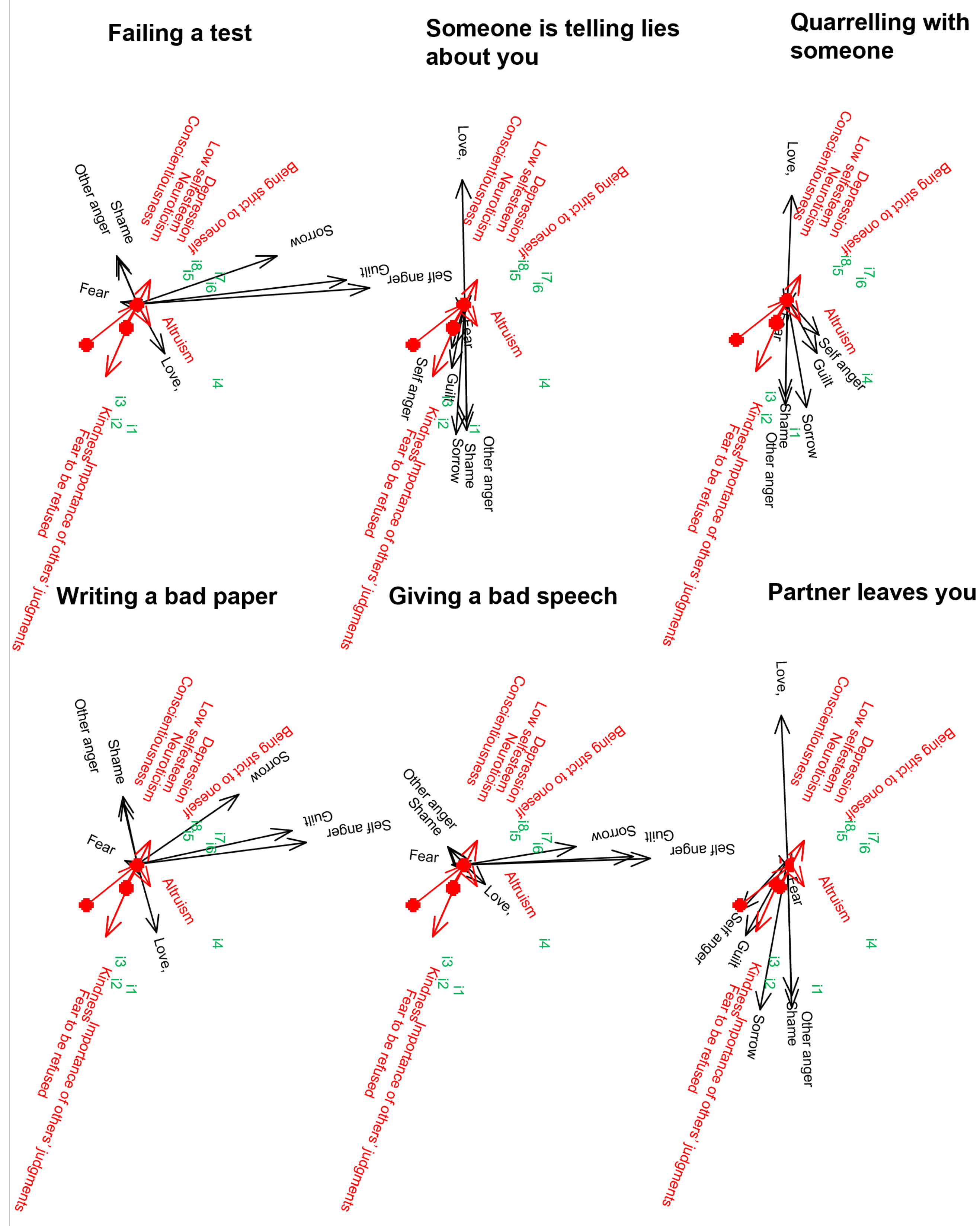

Table 1.
This is a table caption. Tables should be placed in the main text near to the first time they are cited.
Table 1.
This is a table caption. Tables should be placed in the main text near to the first time they are cited.
| Eigenvalue | Exp. Var % | Cummulative % | |
|---|---|---|---|
| Comp. 1 | 6.98 | 38.56 | 38.56 |
| Comp. 2 | 5.28 | 28.45 | 67.01 |
Table 2.
Component values for the situations, resulting from the Bin-3-Way-PARAFAC-PLS (values exceeding 0.4 in absolute value are in bold)
Table 2.
Component values for the situations, resulting from the Bin-3-Way-PARAFAC-PLS (values exceeding 0.4 in absolute value are in bold)
| Situation | Comp. 1 | Comp. 2 |
|---|---|---|
| Quarrelling with someone | -0.45 | -0.09 |
| Partner leaves you | -0.62 | 0.14 |
| Someone is telling lies about you | -0.53 | 0.04 |
| Giving a bad speech | 0.08 | -0.54 |
| Failing a test | 0.21 | -0.67 |
| Writing a bad paper | 0.29 | -0.49 |
Table 3.
Component matrix for the response scales, resulting from the Bin-3-Way-PARAFAC-PLS (values exceeding 0.4 in absolute value are in bold)
Table 3.
Component matrix for the response scales, resulting from the Bin-3-Way-PARAFAC-PLS (values exceeding 0.4 in absolute value are in bold)
| Response | Comp. 1 | Comp. 2 |
|---|---|---|
| Other anger | -0.48 | 0.06 |
| Shame | -0.45 | 0.06 |
| Love | 0.48 | -0.08 |
| Sorrow | -0.49 | -0.40 |
| Fear | -0.04 | 0.05 |
| Guilt | -0.25 | -0.61 |
| Self anger | -0.16 | -0.67 |
Table 4.
Measures of fit for columns
| Deviance | D.F. | P-val | Nagelkerke | Cox-Snell | McFadden | % Correct | |
|---|---|---|---|---|---|---|---|
| Fear of rejection | 6.47 | 2 | 0.04 | 0.76 | 0.55 | 0.61 | 87.5 |
| Kindness | 6.47 | 2 | 0.04 | 0.76 | 0.55 | 0.61 | 87.5 |
| Importance of others’judgments | 6.47 | 2 | 0.04 | 0.76 | 0.55 | 0.61 | 87.5 |
| Altruism | 0.47 | 2 | 0.79 | 0.08 | 0.06 | 0.04 | 50.0 |
| Neuroticism | 6.71 | 2 | 0.03 | 0.77 | 0.57 | 0.63 | 87.5 |
| Being strict to oneself | 3.96 | 2 | 0.14 | 0.58 | 0.39 | 0.44 | 75.0 |
| Low self esteem | 6.71 | 2 | 0.03 | 0.77 | 0.57 | 0.63 | 87.5 |
| Conscientiousness | 6.71 | 2 | 0.03 | 0.77 | 0.57 | 0.63 | 87.5 |
| Depression | 6.71 | 2 | 0.03 | 0.77 | 0.57 | 0.63 | 87.5 |
| Total | 50.71 | 18 | 0.00 | 0.69 | 0.51 | 0.54 | 81.94 |
Abbreviations: Deviance: Deviance statistic; D.F.: Degrees of freedom; P-val: p-value; Nagelkerke: Nagelkerke pseudo-R²; Cox-Snell: Cox-Snell pseudo-R²; McFadden: McFadden pseudo-R²; % Correct: Percentage of correct predictions.
Disclaimer/Publisher’s Note: The statements, opinions and data contained in all publications are solely those of the individual author(s) and contributor(s) and not of MDPI and/or the editor(s). MDPI and/or the editor(s) disclaim responsibility for any injury to people or property resulting from any ideas, methods, instructions or products referred to in the content. |
© 2025 by the authors. Licensee MDPI, Basel, Switzerland. This article is an open access article distributed under the terms and conditions of the Creative Commons Attribution (CC BY) license (http://creativecommons.org/licenses/by/4.0/).
Copyright: This open access article is published under a Creative Commons CC BY 4.0 license, which permit the free download, distribution, and reuse, provided that the author and preprint are cited in any reuse.


