Submitted:
30 June 2025
Posted:
01 July 2025
You are already at the latest version
Abstract
This article investigates the impact of five optimization approximation algorithms on our previously introduced Boolean-Hamiltonians Transform for Quantum Approximate Optimization Algorithm (BHT-QAOA) using two performance metrics. These algorithms are BFGS, L-BFGS-B, SLSQP, COBYLA, and COBYQA. The performance of such an impact is evaluated and compared using two metrics: the final number of function evaluations for an algorithm, and the final quality of qubits measurement for all best-approximated solutions for a problem. A set of arbitrary classical Boolean problems in various logical structures was examined and evaluated using BHT-QAOA, five approximation algorithms, and an IBM quantum computer. Broadly, the BHT-QAOA with these five classical approximation algorithms successfully finds all optimized approximated solutions for these problems. Specifically, both BFGS and SLSQP approximation algorithms successfully search for all best-approximated solutions for these problems, in the context of fewer number of function evaluations and higher quality of qubits measurement, in the hybrid classical-quantum domain.
Keywords:
Boolean oracles
; Hamiltonians
; optimization
; approximation algorithms
; QAOA
1. Introduction
In quantum computing, to solve combinatorial optimization problems, such as the MaxCut [1,2], the quantum approximate optimization algorithm (QAOA) was introduced by Farhi et al. [3,4]. The QAOA represents a combinatorial optimization problem in the form of an ansatz Hamiltonian oracle, which is the so-called “Hamiltonian clauses (HC)”, and an ansatz Hamiltonian operator, which is the so-called “Hamiltonian mixer (HM)”. Note that the wording “ansatz” means that HC and HM consist of parameterized rotational quantum gates of Pauli-Z (RZ) and Pauli-X (RX), respectively [3,4]. Such that HC consists of a number of RZ(v⋅ɣ), RZZ(v⋅ɣ), RZZZ(v⋅ɣ), and so on, while HM consists of n numbers of RX(ω⋅β), where (i) v and ω are the coefficients of time evolutions, (ii) ɣ and β are the parameterized angular rotations between the angles of [0, 2π] and [0, π], respectively [3,4], and (iii) n is the number of input qubits for a problem initially set to the states of |0⟩.
In the quantum domain, HC is the circuit of a problem as the unitary operator , which is a set of non-connected nodes as RZj(v⋅ɣ) and connected nodes as RZjZk(v⋅ɣ), where j and k are the indices of input qubits. While HM is the circuit for the sum of all n input qubits as the unitary operator , which is a set of n RX(ω⋅β). Notice that HM acts as the diffusion operator of QAOA analogous to the diffusion operator in Grover’s search algorithm [5,6,7,8], and HM may include other variants and types of gates, not just RX gates, depending on the model of QAOA used [9,10,11,12,13]. To improve the quality of all approximated solutions, HC and HM are iterated for a number of repetitions (p), where p ≥ 1. Such that every consists of RZ(v⋅ɣp), RZZ(v⋅ɣp), etc., and every consists of RX(ω⋅βp).
In the classical domain, the numerical values of coefficients (v and ω) are calculated during the construction of HC and HM. The numerical values of angles (ɣ and β) are initially randomized as [ɣ1 … ɣp, β1 … βp] for HC and HM, respectively. Notice that some studies initialized such angles to defined values using machine learning and tensor techniques [9,10,11,12,13]. In general, the circuit of QAOA is executed with a quantum processing unit (QPU), and then measured (in the classical domain) for approximated solutions depending on the chosen values of ɣ and β. The measured solutions (as the energy cost of QAOA [3,4]), the chosen values of ɣ and β (as the optimization parameters of QAOA), and the Hamiltonians (HC and HM as an objective function) are fed to a classical optimization minimizer function [14,15,16]. Such a minimizer then recalculates the numerical values of these optimization parameters based on the energy cost from the objective function, and updates HC and HM of QAOA with new optimized numerical values of ɣ and β, respectively. For a number of objective function evaluations (nfev), the optimization operational concurrencies between a QPU and a minimizer are repeated, until finding all optimized approximated solutions for a combinatorial optimization problem or stopping based on a pre-defined condition, which is the so-called “halt condition”. For that, the QAOA is considered a variational quantum search algorithm solving combinatorial optimization problems, in the hybrid classical-quantum domain [17,18,19].
In our work [20], we introduced a new methodology for solving arbitrary classical Boolean problems as Hamiltonians (HC and HM) using QAOA, and we termed this new variant of QAOA the “Boolean-Hamiltonians Transform for QAOA (BHT-QAOA)”. In general, the BHT-QAOA can be summarized as follows.
- An arbitrary classical Boolean problem is constructed as a quantum Boolean oracle [8,21]. This constructed oracle can be expressed in arbitrary logical structures, such as Product-Of-Sums (POS) [22,23], Sum-Of-Products (SOP) [22,24], Exclusive-or Sum-Of-Products (ESOP) [25,26], XOR-Satisfiability (CNF-XOR SAT and DNF-XOR SAT) [27,28], Algebraic Normal Form (ANF) (or Reed-Muller expansion) [29,30], just to name a few.
- This constructed oracle (in any logical structure) is converted into its equivalent quantum Boolean oracle in ESOP structure, unless it was initially constructed in ESOP structure.
- The Hamiltonians (HC and HM) of QAOA are then generated from this transformed quantum Phase oracle, based on our modified composition rules originally presented by Hadfield [31].
- The above-mentioned optimization operational concurrencies between a QPU and a minimizer are performed for the generated HC and HM, until finding all optimized approximated solutions. Notice that, in [20], the SciPy optimization minimizer [32] is performed using the constrained optimization by linear approximation (COBYLA) algorithm [14,16,32].
The goal of this article is to investigate various approximation algorithms of SciPy optimization minimizer for the BHT-QAOA to find all optimized approximated solutions for arbitrary classical Boolean problems. These optimization approximation algorithms are: (i) Broyden-Fletcher-Goldfarb-Shanno (BFGS) [32,33,34], (ii) limited-memory BFGS with bounds (L-BFGS-B) [35,36], (iii) sequential least squares programming (SLSQP) [37,38], (iv) COBYLA, and (v) constrained optimization by quadratic approximations (COBYQA) [39]. Our investigation is comparing and classifying such approximation algorithms based on our two proposed performance metrics: (i) the final utilization of nfev and (ii) the final quality of qubits measurement as the optimized approximated solutions.
In this article, arbitrary classical Boolean problems (as applications) are expressed as Boolean oracles in various logical structures, and these Boolean oracles are then solved using BHT-QAOA for p repetitions, with an IBM QPU and different algorithms of SciPy optimization minimizer. These applications are: (i) an arbitrary Boolean problem in POS structure, (ii) an arbitrary Boolean problem in SOP structure, (iii) an arbitrary Boolean problem in ESOP structure, (iv) a 2×2 Sudoku game, and (v) a 4-bit conditioned half-adder digital circuit. Eventually, our investigation proves that the BFGS and SLSQP algorithms for the BHT-QAOA successfully find all best-approximated solutions for these arbitrary applications, in the context of fewer nfev and higher quality of qubits measurement.
2. Methods
In quantum computing, a quantum Boolean oracle is an easier and straightforward approach in conceptually expressing an arbitrary classical Boolean problem than using a quantum Phase oracle, because (i) the quantum Boolean-based gates can be easily realized using the truth tables (and De Morgan’s Laws [22]) of their equivalent classical Boolean gates, and (ii) the quantum Boolean-based gates and their qubits can be easily analyzed using classical Boolean logic, such as a Boolean logic of 0 represents a quantum state of |0⟩ and a Boolean logic of 1 represents a quantum state of |1⟩. In this article, for ease of description, the quantum Boolean oracle and the quantum Phase oracle will be simply denoted as the “Boolean oracle” and the “Phase oracle”, respectively.
In BHT-QAOA, converting a Boolean oracle (in any logical structure) into a Phase oracle will (i) remove all ancilla qubits (including the output qubit), i.e., the total number of utilized qubits will be dramatically reduced to the number of input qubits only, and (ii) omit the mirror gates (as the uncomputing part) of an oracle, i.e., the total number of quantum gates will be significantly minimized for the circuit of a Phase oracle, depending on the initial construction of a Boolean oracle that expresses a classical Boolean problem.
2.1. The Methodology of BHT-QAOA
Our essential methodology [20] of BHT-QAOA for solving arbitrary classical Boolean problems in the hybrid classical-quantum domain can be simply discussed as follows. Firstly, a classical Boolean problem is conceptually designed as a Boolean oracle in any logical structure. Such an oracle may consist of n input qubits (as the literals of a Boolean expression or the variables of a problem), m ancilla qubits (as the auxiliary output qubits) for intermediate quantum operations, and one fqubit (as the functional qubit) for the final quantum output of this oracle, where n ≥ 2 and m ≥ 0.
Secondly, this Boolean oracle in any logical structure is converted into its equivalent Boolean oracle in ESOP structure. There are many synthesis methods to achieve such a conversion, such as ESOP synthesis [25], Karnaugh map synthesis [22], binary decision diagram (BDD) synthesis [40,41], just to name a few. By utilizing any synthesis method, all mirror gates and m ancillae (except fqubit) are removed for the converted Boolean oracle in ESOP structure. Notice that a synthesis method may not generate the minimized ESOP structure; however, the DSOP (Disjoint Sum-Of-Products) structure may be generated, which is an expensive structure as compared to the minimized ESOP structure, depending on the number of n-bit Toffoli gates, where n ≥ 3 qubits.
Thirdly, this Boolean oracle in ESOP (or DSOP) structure is transformed into its equivalent Phase oracle, by utilizing the technique originally discussed by Figgatt et al. [21] for transforming 4-bit Toffoli gates into 3-bit controlled-Z (CCZ) gates, for Grover’s algorithm of single-solution [5,6,7,8]. In [20], we efficiently generalized their technique to include Feynman (CX) and n-bit Toffoli gates as well, and we termed our generalized technique the “generalized transformation rules” as follows.
| Rule 1: | A Feynman (CX) gate is transformed into a Pauli-Z (Z) gate, when Equation (1) stated below is a solution-satisfiable, where j is the index of an input qubit (q). The left side of Equation (1) is the Boolean-based output of a CX gate, and its right side is the phase-inverted output of a Z gate. | |
|
|
(1) | |
| Rule 2: | A Toffoli gate is transformed into a controlled-Z (CZ) gate, when Equation (2) stated below is a solution-satisfiable, where j and k are the indices of input qubits (q). The left side of Equation (2) is the Boolean-based output of a Toffoli gate, and its right side is the phase-inverted output of a CZ gate. | |
|
|
(2) | |
| Rule 3: | An n-bit Toffoli gate is transformed into an (n–1)-bit multi-controlled Z (MCZ) gate, when Equation (3) stated below is a solution-satisfiable, where j is the index of an input qubit (q) and n ≥ 3 qubits (q + fqubit). The left side of Equation (3) is the Boolean-based output of an n-bit Toffoli gate, and its right side is the phase-inverted output of an (n–1)-bit MCZ gate. | |
|
|
(3) | |
After applying these generalized transformation rules on the Boolean oracle in ESOP (or DSOP) structure, the resultant circuit of Phase oracle is simply constructed, with the removal of fqubit, i.e., the width of a circuit is reduced, and the significant minimization of multi-controlled quantum gates, i.e., the depth of a circuit is shrunk.
Fourthly, the Hamiltonians (HC and HM) of BHT-QAOA are directly generated from the converted Phase oracle, using our four proposed “generalized composition rules (Hg)” stated in Table 1, which are generalized from three Hadfield’s Boolean-based composition rules (Hf) [31] for the quantum Boolean-based gates of Feynman (CX), 3-bit Toffoli (CCX), and n-bit Toffoli (). In Table 1, four quantum gates are mainly utilized to generate the Hamiltonians (HC and HM) from a Phase oracle, using the quantum phase-based gates of Pauli-Z (Z), controlled-Z (CZ), multi-controlled Z (MCZ), and Pauli-X (X).
Finally, based on Table 1, the four generalized composition rules (Hg) will be then directly applied to a Phase oracle to generate HC and calculate its v coefficient. Because β (as a set of rotational angles of HM) rotates between [0, π] [3,4], we set its coefficient (ω) to cover all the range between [0, 2π] for possible phase values of RX gates in HM, to find all optimized approximated solutions for an arbitrary classical Boolean problem. Such that, ω (as the coefficient of β) is initially set to 2 for all n numbers of RX(ω⋅β) gates in HM, where n is the total number of input qubits.
2.2. The Architecture of BHT-QAOA
After transforming an arbitrary classical Boolean problem to the Hamiltonians (HC and HM) and calculating their coefficients (v and ω), respectively, the numerical values of ɣ and β are initially randomized and then plugged into the architecture of BHT-QAOA for first execution, as illustrated in Figure 1. Subsequently, the SciPy optimization minimizer is utilized to optimize these numerical values (ɣ and β) for best-approximated solutions, in a number of function evaluations (nfev), by employing three cofactors as follows.
- HC and HM (in a number of p), as the “objective function” needs to be minimized.
- Measured solutions of BHT-QAOA, as the “energy cost” of the objective function.
- Previously calculated ɣ and β, as their “numerical values” need to be optimized.
2.3. The Optimization Approximation Algorithms
In our research of the BHT-QAOA [20], we utilized the SciPy optimization minimizer and COBYLA algorithm with promising optimized approximated solutions for arbitrary classical Boolean problems. However, in this article, we investigate other approximation algorithms for the BHT-QAOA. These optimization approximation algorithms are BFGS, L-BFGS-B, SLSQP, COBYLA, and COBYQA. Our investigation is based on the comparison among these five optimization approximation algorithms using our two performance metrics, which are the final utilization of nfev and the final quality of qubits measurement as the best-approximated solutions. Notice that, after measurement, qubits are converted into bits, and the quality of qubits measurement indicates that the solutions become more distinguishable from the non-solutions.
The Broyden-Fletcher-Goldfarb-Shanno (BFGS) algorithm [32,33,34] is an iterative quasi-Newton method [38] for solving unconstrained nonlinear optimization problems. The BFGS iteratively approximates the Hessian matrix [38,39] to find the minimum of a function, often requiring fewer iterations than the gradient descent (GD) algorithm [38]. The BFGS is widely used in machine learning (ML) [42] for training models, such as neural networks (NN) [43] and support vector machines (SVM) [44].
The limited-memory BFGS with bounds (L-BFGS-B) algorithm [35,36] is a limited-memory quasi-Newton method to solve large-scale bound-constrained nonlinear optimization problems. The L-BFGS-B is mainly utilized for large dense problems and when there is difficulty in computing the Hessian matrix. The L-BFGS-B extends the standard L-BFGS algorithm [45] by incorporating simple bounds (lower and upper limits) on the variables for a function.
The sequential least squares programming (SLSQP) algorithm [37,38] is a method for solving nonlinear optimization problems with constraints. The SLSQP iteratively solves a sequence of quadratic programming subproblems to find the optimal solutions. The SLSQP is particularly useful for problems with both equality and inequality constraints.
The constrained optimization by linear approximation (COBYLA) algorithm [14,16,32] is a derivative-free optimization algorithm for solving problems with nonlinear inequality and equality constraints. COBYLA works by approximating the objective functions and their constraints using linear models, to find solutions without requiring the derivatives of these functions, where their gradients are difficult to compute.
The constrained optimization by quadratic approximations (COBYQA) algorithm [39] is a derivative-free optimization algorithm for solving general nonlinear optimization problems. COBYQA replaces COBYLA as a general derivative-free optimization solver, since COBYQA can handle unconstrained, bound-constrained, linearly constrained, and nonlinearly constrained problems.
3. Results and Discussion
Arbitrary classical Boolean problems (applications) are designed as Boolean oracles (in different logical structures). These Boolean oracles are solved with the BHT-QAOA for p repetitions, where p ≥ 1. As shown in Figure 1, our experiments have utilized the ibm_brisbane [46] QPU to perform the quantum processing domain of the BHT-QAOA, to execute the quantum circuit of an application, in p. While the SciPy minimizer performs the classical processing domain of the BHT-QAOA, to optimize the numerical values of ɣ and β with the energy cost of their Hamiltonians (HC and HM), in nfev. These applications are investigated using five optimization approximation algorithms of SciPy minimizer function, which are BFGS, L-BFGS-B, SLSQP, COBYLA, and COBYQA.
Because of our IBM Quantum Platform account limitations, the complete architecture of BHT-QAOA (shown in Figure 1) is completely simulated in the classical domain using IBM quantum libraries (Qiskit, AerSimulator, and Aer-EstimatorV2 [46,47,48]), for 1024 resampling times, which is the so-called “shots” [49]. After this classically simulated BHT-QAOA, the optimized numerical values of ɣ and β (from the SciPy minimizer with five approximation algorithms) are concurrently plugged into their respective HC and HM for an application, using the simulated noisy model of the ibm_brisbane QPU.
Notice that due to the limited physical connectivity of four neighboring qubits for the recent quantum layouts (architectures) of IBM QPUs [50,51], the designed Boolean oracles (in various logical structures) for the following applications must have n input qubits and m ancilla qubits (including fqubit), where 2 ≤ n ≤ 4 and m ≥ 0. Figure 2 demonstrates the circuits of Boolean oracles for these applications as follows.
- An arbitrary Boolean problem in POS structure, as stated in Equation (4) and shown in Figure 2a.
(a ∨ b ∨ ¬ c) ∧ (¬ a ∨ c) ∧ (¬ b ∨ c)
- 2.
- An arbitrary Boolean problem in SOP structure, as stated in Equation (5) and illustrated in Figure 2b.
(a ∧ b ∧ ¬ c) ∨ ( ¬ a ∧ c) ∨ ( ¬ b ∧ c)
- 3.
- An arbitrary Boolean problem in ESOP structure, as stated in Equation (6) and shown in Figure 2c.
(a ∧ b ∧ ¬ c) ⊕ (¬ a ∧ c) ⊕ (¬ b ∧ c)
- 4.
(cell1 ⊕ cell2) ∧ (cell1 ⊕ cell3) ∧ (cell2 ⊕ cell4) ∧ (cell3 ⊕ cell4)
- 5.
- A 4-bit conditioned half-adder (HA) digital circuit, which is ORing two 1-bit sums and then ANDing them with one 1-bit carry-out, as stated in Equation (8) and illustrated in Figure 2e,f.
[(a0 ⊕ b0) ∨ ((a0 ∧ b0) ⊕ (a1 ⊕ b1))] ∧ [(a1 ∧ b1) ∨ ((a0 ∧ b0) ∧ (a1 ⊕ b1))]
For the two performance metrics (the final utilization of nfev and the final quality of qubits measurement), Table 2 states the comparison of the final utilization of nfev for the five optimization approximation algorithms for all applications. While Figure 3 illustrates the final measured solutions (as the quality of qubits measurement) for all applications using the five optimization approximation algorithms.
As illustrated in Figure 3(a–e), the highest bars in the histograms denote the final solutions for all applications using the five optimization approximation algorithms, and each histogram of an application denotes the results of (a) four solutions {, , , } for the Boolean oracle in POS structure of Equation (4), (b) four solutions { , , , } for the Boolean oracle in SOP structure of Equation (5), (c) three solutions {, , } for the Boolean oracle in ESOP structure of Equation (6), (d) two permutative solutions {solution 1: cell1=cell4=0 and cell2=cell3=1; solution 2: cell1=cell4=1 and cell2=cell3=0} for the 2×2 Sudoku game of Equation (7), and (e) three solutions {, , } for the 4-bit conditioned half-adder (HA) circuit of Equation (8).
Notice that, in Figure 3, (i) the first measured bit (the most-right) of a solution is equivalent to the first input qubit, (ii) the last measured bit (the most-left) of a solution is equivalent to the last input qubit, (iii) the higher probability of qubits indicates a solution, and (iv) the lower probability of qubits indicates a non-solution. Table 3 summarizes the final quality of qubits measurement for all optimization approximation algorithms with the BHT-QAOA, as calculated in Equation (9), where N = , n is the number of input qubits, S is the probability of a solution, and P is the probability of a solution or non-solution.
Based on the evaluation of two performance metrics in Table 2 and Table 3, on the one hand, the BHT-QAOA successfully optimizes the numerical values of ɣ and β and finds all approximated solutions for all applications, as a proof of concept for utilizing any optimization approximation algorithm with the BHT-QAOA to solve arbitrary classical Boolean problems. On the other hand, the BFGS and SLSQP are the fastest optimization approximation algorithms for the BHT-QAOA, in the context of fewer utilization of nfev. While the BFGS, L-BFGS-B, and SLSQP are the most accurate optimization approximation algorithms for the BHT-QAOA, in the context of a higher quality of qubits measurement. Broadly, the BFGS and SLSQP algorithms successfully demonstrate their capabilities of optimizing the numerical values of ɣ and β and find all best-approximated solutions for all applications, as compared to the other utilized optimization approximation algorithms.
Accordingly, the BHT-QAOA with the BFGS and SLSQP algorithms will provide broad opportunities in investigating many of classical Boolean problems in the hybrid classical-quantum domain, which are neither designed nor solved using the standard QAOA [3,4]. Therefore, various classical Boolean problems for the applications of digital logic circuits, synthesizers, and machine learning can be realized as Hamiltonians and then solved using BHT-QAOA with these two optimization approximation algorithms.
4. Conclusions
Our previously introduced BHT-QAOA (Boolean-Hamiltonians Transform for Quantum Approximate Optimization Algorithm [20]), to solve arbitrary classical Boolean problems as Hamiltonians in the hybrid classical-quantum domain, is re-investigated with five classical optimization approximation algorithms and two performance metrics. These algorithms are BFGS, L-BFGS-B, SLSQP, COBYLA, and COBYQA. While the two performance metrics are: (i) the final utilization of nfev and (ii) the final quality of qubits measurement for the best-approximated solutions, where nfev is the number of function evaluations for a problem between a quantum processing unit and a classical optimization approximation algorithm.
In this article, arbitrary Boolean applications are constructed as Boolean oracles in various logical structures, and then BHT-QAOA successfully searches for all optimized approximated solutions for these applications using all five optimization approximation algorithms, in the hybrid classical-quantum domain. However, our investigation proved that the BFGS and SLSQP are the fastest optimization approximation algorithms for the BHT-QAOA, in the context of fewer utilization of nfev. While the BFGS, L-BFGS-B, and SLSQP are the most accurate optimization approximation algorithms for the BHT-QAOA, in the context of a higher quality of qubits measurement. Collectively, both BFGS and SLSQP approximation algorithms successfully demonstrate their capabilities in finding all best-approximated solutions for these arbitrary Boolean applications, in the context of both fewer values of nfev and higher quality of qubits measurement.
In conclusion, further classical Boolean problems can be investigated for arbitrary logical structures for the practical engineering applications in the topics of digital logic synthesizers, robotics, machine learning, just to name a few, and the BHT-QAOA with the BFGS and SLSQP algorithms will successfully solve such practical applications effectively in the hybrid classical-quantum domain.
Author Contributions
Conceptualization, A.A.; Methodology, A.A.; Formal analysis, A.A. and M.P.; Writing—original draft preparation, A.A.; Visualization, A.A.; Supervision, A.A. and M.P. All authors have read and agreed to the published version of the manuscript.
Funding
This research received no external funding.
Institutional Review Board Statement
Not applicable.
Data Availability Statement
The original contributions presented in our study are included in this article, further inquiries can be directed to the corresponding author (A.A.).
Conflicts of Interest
The authors declare no conflicts of interest.
References
- Goemans, M.X.; Williamson, D.P. .878-approximation algorithms for max cut and max 2sat. In Proc. of the Twenty-Sixth Ann. ACM Symp. on Theory of Computing, 1994, pp. 422–431.
- Rendl, F.; Rinaldi, G.; Wiegele, A. Solving max-cut to optimality by intersecting semidefinite and polyhedral relaxations. Mathematical Programming 2010, 121, 307–335. [Google Scholar] [CrossRef]
- Farhi, E.; Goldstone, J.; Gutmann, S. A quantum approximate optimization algorithm. arXiv Preprint 2014. [Google Scholar] [CrossRef]
- Farhi, E.; Goldstone, J.; Gutmann, S.; Neven, H. Quantum algorithms for fixed qubit architectures. arXiv Preprint 2017. [Google Scholar] [CrossRef]
- Grover, L.K. A fast quantum mechanical algorithm for database search. In Proc. of the 28th Ann. ACM Symp. on Theory of Computing, 1996, pp. 212–219.
- Grover, L.K. Quantum mechanics helps in searching for a needle in a haystack. Physical Review Letters 1997, 79, 325. [Google Scholar] [CrossRef]
- Grover, L.K. A framework for fast quantum mechanical algorithms. In Proc. of the 30th Ann. ACM Symp. on Theory of Computing, 1998, pp. 53–62.
- Al-Bayaty, A.; Perkowski, M. A concept of controlling Grover diffusion operator: a new approach to solve arbitrary Boolean-based problems. Scientific Reports 2024, 14, 23570. [Google Scholar] [CrossRef]
- Moussa, C.; Wang, H.; Bäck, T.; Dunjko, V. Unsupervised strategies for identifying optimal parameters in quantum approximate optimization algorithm. EPJ Quantum Technology 2022, 9, 11. [Google Scholar] [CrossRef]
- Amosy, O.; Danzig, T.; Lev, O.; Porat, E.; Chechik, G.; Makmal, A. Iteration-free quantum approximate optimization algorithm using neural networks. Quantum Machine Intelligence 2024, 6, 38. [Google Scholar] [CrossRef]
- Herrman, R.; Lotshaw, P.C.; Ostrowski, J.; Humble, T.S.; Siopsis, G. Multi-angle quantum approximate optimization algorithm. Scientific Reports 2022, 12, 6781. [Google Scholar] [CrossRef]
- Wurtz, J.; Lykov, D. Fixed-angle conjectures for the quantum approximate optimization algorithm on regular MaxCut graphs. Physical Review A 2021, 104, 052419. [Google Scholar] [CrossRef]
- Crooks, G.E. Performance of the quantum approximate optimization algorithm on the maximum cut problem. arXiv Preprint 2018. [Google Scholar] [CrossRef]
- Fernández-Pendás, M.; Combarro, E.F.; Vallecorsa, S.; Ranilla, J.; Rúa, I. F. A study of the performance of classical minimizers in the quantum approximate optimization algorithm. Journal of Computational and Applied Mathematics 2022, 404, 113388. [Google Scholar] [CrossRef]
- Powell, M.J.D. Advances in Optimization and Numerical Analysis; Gomez, S., Hennart, J.P., Eds.; Springer: Dordrecht, The Netherlands, 1994; pp. 51–67. [Google Scholar]
- Powell, M.J.D. A view of algorithms for optimization without derivatives. Mathematics Today-Bulletin of the Institute of Mathematics and its Applications 2007, 43, 170–174. [Google Scholar]
- Cerezo, M.; Arrasmith, A.; Babbush, R.; Benjamin, S.C.; Endo, S.; Fujii, K.; McClean, J.R.; Mitarai, K.; Yuan, X.; Cincio, L.; Coles, P.J. Variational quantum algorithms. Nature Reviews Physics 2021, 3, 625–644. [Google Scholar] [CrossRef]
- Wecker, D.; Hastings, M. B.; Troyer, M. Progress towards practical quantum variational algorithms. Physical Review A 2015, 92, 042303. [Google Scholar] [CrossRef]
- Tilly, J.; Chen, H.; Cao, S.; Picozzi, D.; Setia, K.; Li, Y.; Grant, E.; Wossnig, L.; Rungger, I.; Booth, G.H.; Tennyson, J. The variational quantum eigensolver: a review of methods and best practices. Physics Reports 2022, 986, 1–128. [Google Scholar] [CrossRef]
- Al-Bayaty, A.; Perkowski, M. BHT-QAOA: the generalization of quantum approximate optimization algorithm to solve arbitrary Boolean problems as Hamiltonians. Entropy 2024, 26, 843. [Google Scholar] [CrossRef]
- Figgatt, C.; Maslov, D.; Landsman, K.A.; Linke, N.M.; Debnath, S.; Monroe, C. Complete 3-qubit Grover search on a programmable quantum computer. Nature Communications 2017, 8, 1918. [Google Scholar] [CrossRef]
- Wakerly, J.F. Digital Design: Principles and Practices, 4th ed.; Pearson Education: New Delhi, India, 2014. [Google Scholar]
- Zhang, L.X.; Huang, W. A note on the invariance principle of the product of sums of random variables. Electronic Communications in Probability 2007, 12, 59–64. [Google Scholar]
- Zimmermann, R.; Tran, D.Q. Optimized synthesis of sum-of-products. In IEEE Thirty-Seventh Asilomar Conf. on Signals, Systems & Computers, 2003, pp. 867–872.
- Mishchenko, A.; Perkowski, M. Fast heuristic minimization of exclusive sums-of-products. In Proc. RM’2001 Workshop, 2001, pp. 242–250.
- Sasao, T. EXMIN2: a simplification algorithm for exclusive-or-sum-of-products expressions for multiple-valued-input two-valued-output functions. IEEE Trans. on Computer-Aided Design of Integrated Circuits and Systems 1993, 12, 621–632. [Google Scholar] [CrossRef]
- Ibrahimi, M.; Kanoria, Y.; Kraning, M.; Montanari, A. The set of solutions of random XORSAT formulae. In Proc. of the 23rd Ann. ACM-SIAM Symp. on Discrete Algorithms, 2012, pp. 760–779.
- Soos, M.; Meel, K.S. BIRD: engineering an efficient CNF-XOR SAT solver and its applications to approximate model counting. In Proc. of the AAAI Conf. on Artificial Intelligence, 2019, 33, pp. 1592–1599.
- Stankovic, R.S.; Sasao, T. A discussion on the history of research in arithmetic and Reed-Muller expressions. IEEE Trans. on Computer-Aided Design of Integrated Circuits and Systems 2001, 20, 1177–1179. [Google Scholar] [CrossRef]
- Kurgalin, S.; Borzunov, S. Concise Guide to Quantum Computing: Algorithms, Exercises, and Implementations; Springer: Cham, Switzerland, 2021; pp. 37–43. [Google Scholar]
- Hadfield, S. On the representation of Boolean and real functions as Hamiltonians for quantum computing. ACM Trans. on Quantum Computing (TQC) 2021, 2, 1–21. [Google Scholar] [CrossRef]
- Lavrijsen, W.; Tudor, A.; Müller, J.; Iancu, C.; De Jong, W. Classical optimizers for noisy intermediate-scale quantum devices. In 2020 IEEE Int. Conf. on Quantum Computing and Engineering (QCE), 2020, pp. 267–277.
- Yuan, Y.X. A modified BFGS algorithm for unconstrained optimization. IMA Journal of Numerical Analysis 1991, 11, 325–332. [Google Scholar] [CrossRef]
- Dai, Y.H. Convergence properties of the BFGS algoritm. SIAM Journal on Optimization 2002, 13, 693–701. [Google Scholar] [CrossRef]
- Zhu, C.; Byrd, R.H.; Lu, P.; Nocedal, J. Algorithm 778: L-BFGS-B: Fortran subroutines for large-scale bound-constrained optimization. ACM Transactions on Mathematical Software (TOMS) 1997, 23, 550–560. [Google Scholar] [CrossRef]
- Liu, D.C.; Nocedal, J. On the limited memory BFGS method for large scale optimization. Mathematical Programming 1989, 45, 503–528. [Google Scholar] [CrossRef]
- Ma, Y.; Gao, X.; Liu, C.; Li, J. Improved SQP and SLSQP algorithms for feasible path-based process optimisation. Computers and Chemical Engineering 2024, 188, 108751. [Google Scholar] [CrossRef]
- Bonnans, J.F.; Gilbert, J.C.; Lemaréchal, C.; Sagastizábal, C.A. Numerical Optimization: Theoretical and Practical Aspects; Springer: Heidelberg, Germany, 2006. [Google Scholar]
- Ragonneau, T.M. Model-Based Derivative-Free Optimization Methods and Software. PhD Thesis, The Hong Kong Polytechnic University, Hong Kong, China, 2022. [Google Scholar]
- Ebendt, R.; Fey, G.; Drechsler, R. Advanced BDD Optimization; Springer: Dordrecht, The Netherlands, 2005. [Google Scholar]
- Wille, R.; Drechsler, R. Effect of BDD optimization on synthesis of reversible and quantum logic. Electronic Notes in Theoretical Computer Science 2010, 253, 57–70. [Google Scholar] [CrossRef]
- Al-Bayaty, A.; Perkowski, M. COVID-19 features detection using machine learning models and classifiers. In The Science behind the COVID Pandemic and Healthcare Technology Solutions; Adibi, S., Rajabifard, A., Shariful Islam, S.M., Ahmadvand, A., Eds.; Springer: Cham, Switzerland, 2022; Volume 15, pp. 379–403. [Google Scholar]
- Zhang, Y.; Mu, B.; Zheng, H. Link between and comparison and combination of Zhang neural network and quasi-Newton BFGS method for time-varying quadratic minimization. IEEE Transactions on Cybernetics 2013, 43, 490–503. [Google Scholar] [CrossRef]
- Li, S.; Tan, M. Tuning SVM parameters by using a hybrid CLPSO–BFGS algorithm. Neurocomputing 2010, 73, 2089–2096. [Google Scholar] [CrossRef]
- Liu, D.C.; Nocedal, J. On the limited memory BFGS method for large scale optimization. Mathematical Programming 1989, 45, 503–528. [Google Scholar] [CrossRef]
- Karimi, N.; Elyasi, S.N.; Yahyavi, M. Implementation and measurement of quantum entanglement using IBM quantum platforms. Physica Scripta 2024, 99, 045121. [Google Scholar] [CrossRef]
- Wille, R.; Van Meter, R.; Naveh, Y. IBM’s Qiskit tool chain: working with and developing for real quantum computers. In 2019 Design, Automation and Test in Europe Conf. & Exhibition (DATE), 2019, pp. 1234–1240.
- Georgopoulos, K.; Emary, C.; Zuliani, P. Modeling and simulating the noisy behavior of near-term quantum computers. Physical Review A 2021, 104, 062432. [Google Scholar] [CrossRef]
- Rao, P.; Yu, K.; Lim, H.; Jin, D.; Choi, D. Quantum amplitude estimation algorithms on IBM quantum devices. In Quantum Communications and Quantum Imaging XVIII, 2020, 11507, pp. 49–60.
- Farrell, R.C.; Illa, M.; Ciavarella, A.N.; Savage, M.J. Scalable circuits for preparing ground states on digital quantum computers: the Schwinger model vacuum on 100 qubits. PRX Quantum 2024, 5, 020315. [Google Scholar] [CrossRef]
- IBM Quantum Platform. Available online: https://quantum.ibm.com/services/resources?tab=systems (accessed on 25 June 2025).
- Simonis, H. Sudoku as a constraint problem. In CP Workshop on Modeling and Reformulating Constraint Satisfaction Problems, 2005, pp. 13-27.
- Lynce, I.; Ouaknine, J. Sudoku as a SAT problem. In Proc. of the 9th Symp. on Artificial Intelligence and Mathematics (AI&M), 2006.
Figure 1.
The architecture of our Boolean-Hamiltonians Transform for QAOA (BHT-QAOA) to solve arbitrary classical Boolean problems as Hamiltonians (HC and HM). The BHT-QAOA is mainly grouped into two processing domains: (i) the classical processing domain as denoted by blue, and (ii) the quantum processing domain as denoted by red [20].
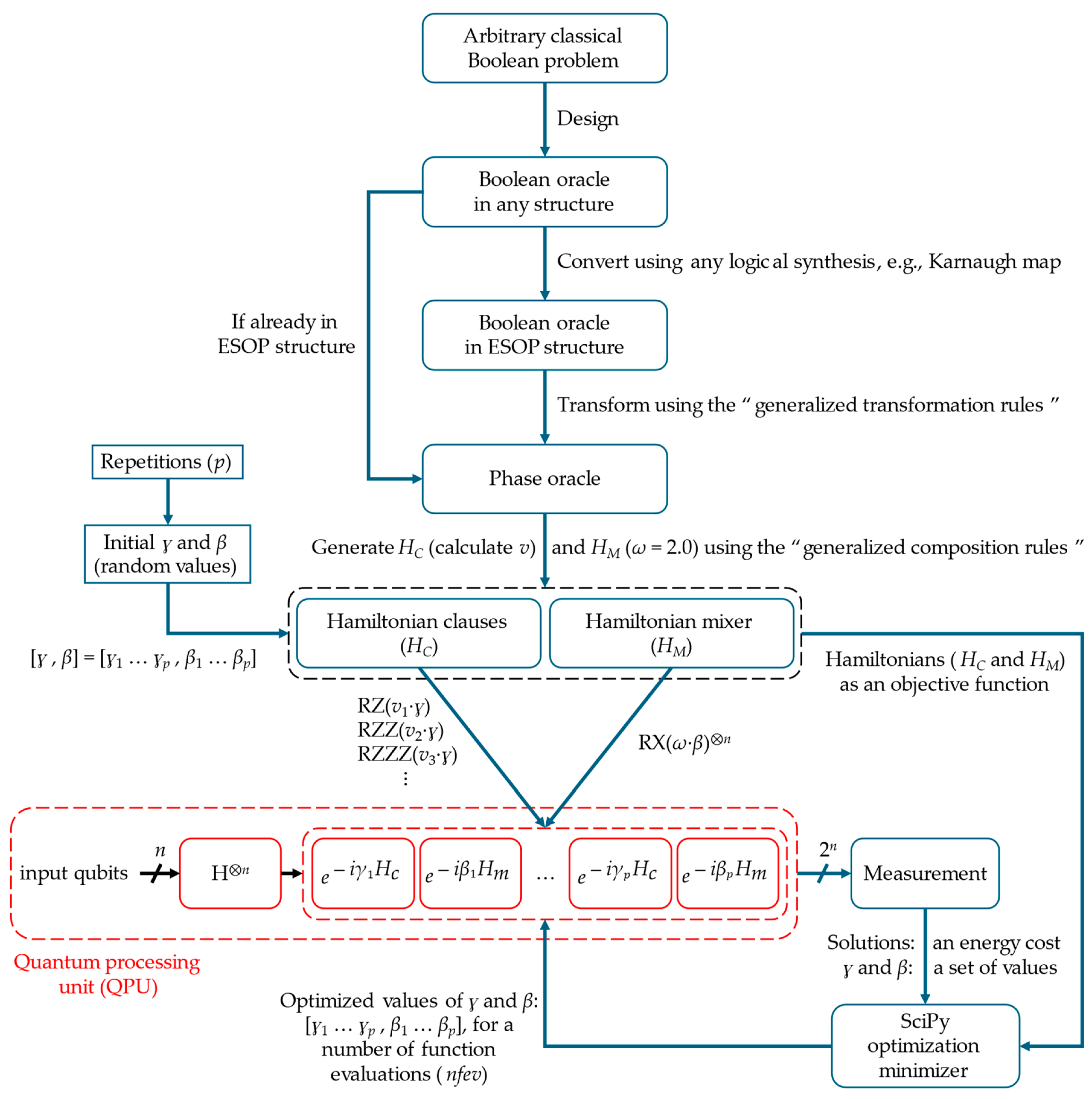
Figure 2.
Schematics of the circuits for arbitrary Boolean problems: (a, upper-left) the Boolean oracle in POS structure representing Equation (4), (b, upper-right) the Boolean oracle in SOP structure representing Equation (5), (c, middle-left) the Boolean oracle in ESOP structure representing Equation (6), (d, middle-right) the Boolean oracle in CNF-XOR SAT structure of 2×2 Sudoku representing Equation (7), (e, bottom-left) the classical 4-bit half-adder (HA) for two 2-bit numbers (A = a1a0 and B = b1b0), and (f, bottom-right) the Boolean oracle in a mixed structure representing Equation (8). All qubits are initially set to the |0⟩ states.
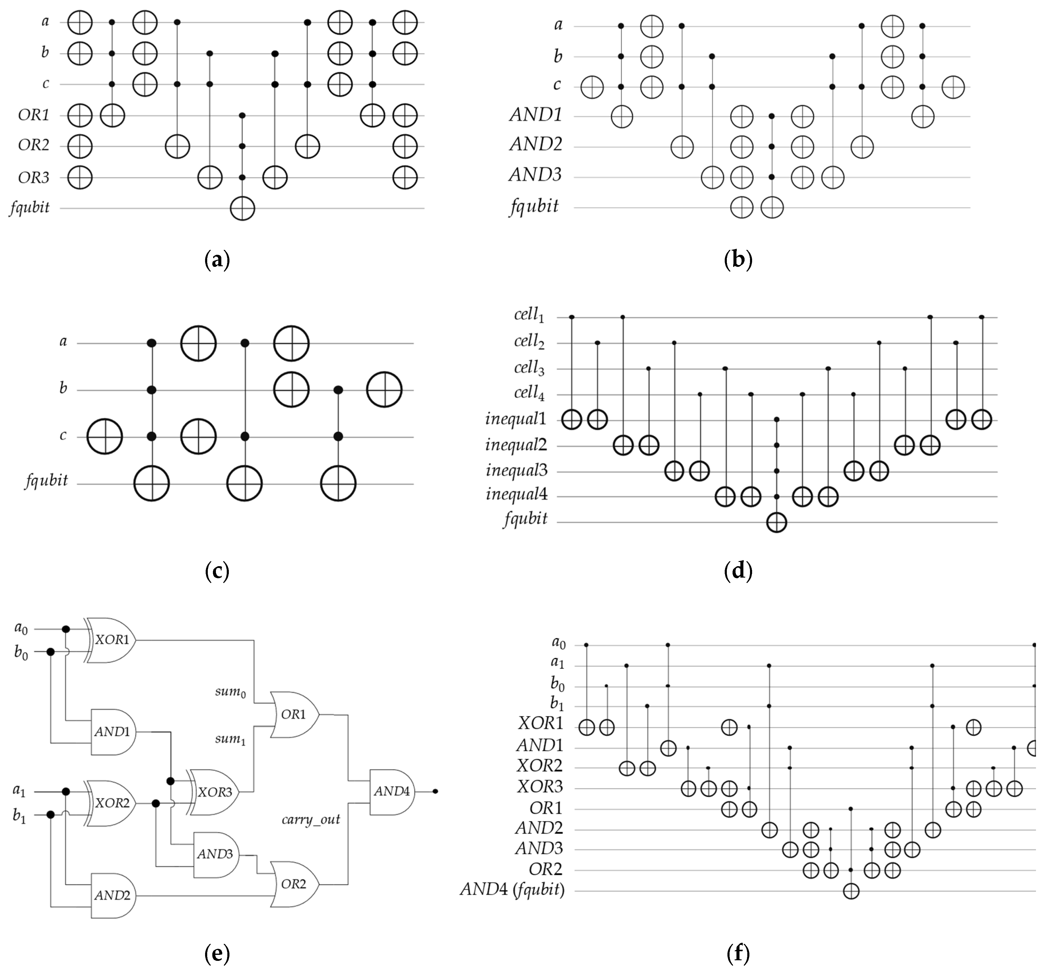
Figure 3.
The final measured solutions (as the quality of qubits measurement performance metric) for all applications executed using five optimization approximation algorithms with the ibm_brisbane QPU (1024 shots): (a, upper-left) the four solutions for the Boolean oracle in POS structure of Equation (4), (b, upper-right) the four solutions for the Boolean oracle in SOP structure of Equation (5), (c, middle-upper) the three solutions for the Boolean oracle in ESOP structure of Equation (6), (d, middle-lower) the two solutions for the 2×2 Sudoku game of Equation (7), and (e, bottom) the three solutions for the 4-bit conditioned HA circuit of Equation (13), where p is the number of repetitions for the quantum circuits of the Hamiltonians (HC and HM) for an application.


Table 1.
Our generalized composition rules (Hg) for Phase oracles, j and k are the indices of input qubits (q), Zj is the RZ gate applied on qj, Q = {qj, qk … qjqk …}, and ZQ = {Zj, Zk … ZjZk …} [20].
Table 1.
Our generalized composition rules (Hg) for Phase oracles, j and k are the indices of input qubits (q), Zj is the RZ gate applied on qj, Q = {qj, qk … qjqk …}, and ZQ = {Zj, Zk … ZjZk …} [20].
| Rules | Gate | Type | g(x) | Hg |
| Rule 1 | Z | Phase |
|
|
| Rule 2 | CZ | Phase |
|
|
| Rule 3 | MCZ | Phase |
|
|
| Rule 4 | X | Phase |
|
Invert signs (±) of all jth qubits in ZQ |
Table 2.
Comparison of the performance metric (the final utilization of nfev) for the five optimization approximation algorithms. The lowest values of nfev are denoted in bold.
Table 2.
Comparison of the performance metric (the final utilization of nfev) for the five optimization approximation algorithms. The lowest values of nfev are denoted in bold.
| Applications | BFGS | L-BFGS-B | SLSQP | COBYLA | COBYQA |
| POS | 27 | 21 | 30 | 49 | 38 |
| SOP | 90 | 185 | 181 | 296 | 165 |
| ESOP | 75 | 100 | 108 | 379 | 123 |
| 2×2 Sudoku | 80 | 115 | 61 | 515 | 124 |
| 4-bit HA circuit | 70 | 85 | 71 | 99 | 93 |
Table 3.
Summary of the performance metric (the final quality of qubits measurement) for the five optimization approximation algorithms. The highest qualities are denoted in bold.
Table 3.
Summary of the performance metric (the final quality of qubits measurement) for the five optimization approximation algorithms. The highest qualities are denoted in bold.
| Applications | BFGS | L-BFGS-B | SLSQP | COBYLA | COBYQA |
| POS | 90.1 | 91.1 | 90.7 | 88.3 | 88.0 |
| SOP | 92.4 | 90.0 | 87.7 | 93.7 | 89.9 |
| ESOP | 85.5 | 87.6 | 86.4 | 80.4 | 80.6 |
| 2×2 Sudoku | 71.8 | 69.8 | 71.3 | 68.7 | 71.7 |
| 4-bit HA circuit | 57.3 | 57.7 | 55.9 | 55.5 | 52.1 |
Disclaimer/Publisher’s Note: The statements, opinions and data contained in all publications are solely those of the individual author(s) and contributor(s) and not of MDPI and/or the editor(s). MDPI and/or the editor(s) disclaim responsibility for any injury to people or property resulting from any ideas, methods, instructions or products referred to in the content. |
© 2025 by the authors. Licensee MDPI, Basel, Switzerland. This article is an open access article distributed under the terms and conditions of the Creative Commons Attribution (CC BY) license (http://creativecommons.org/licenses/by/4.0/).
Copyright: This open access article is published under a Creative Commons CC BY 4.0 license, which permit the free download, distribution, and reuse, provided that the author and preprint are cited in any reuse.


