
Submitted:
04 September 2024
Posted:
05 September 2024
You are already at the latest version
Abstract
This paper aims to outline the effectiveness of modern universal gate quantum computers when utilizing different configurations to solve the B-SAT(Boolean Satisfiability) problem. The quantum computing experiments are performed using Grover’s Search algorithm to find a valid solution. The experiments are performed under different variations to demonstrate their effects on the results. Changing the number of shots, qubit mapping, and using a different quantum processor are all among the experimental variables. The study also branches into a dedicated experiment highlighting a peculiar behavior that IBM quantum processors exhibit when running circuits with a certain number of shots.
Keywords:
quantum computing
; B-SAT
; Boolean satisfiability problem
; Grover’s Search
; electronic design automation (EDA)
; conjunctive normal form (CNF)
; closed box testing
1. Introduction
The applications of quantum computing on electronic design automation (EDA) is an increasingly growing field that is gaining traction as quantum processors improve by the year[1,2]. Universal gate quantum processors are quite efficient at performing tasks that could be parallelized, and closed-box EDA testing has a lot of parallelization potential since it needs to run all possible inputs to verify the function of the digital logical unit. One way to auto-construct a closed-box digital logic unit is to lay it out as a Boolean Satisfiability (B-SAT) problem.
An early application of quantum computers is to solve the Boolean Satisfiability problem using Grover’s Search algorithm[3]. Grover’s search algorithm has long been hailed as one of the flagship algorithms of quantum computing[4]. Its ability to locate an item in an unstructured list has a complexity of: . That being said, quantum computers are far from proving quantum advantage.
While we are still in the noisy intermediate-scale quantum (NISQ) era, various approaches from all angles are being leveraged to achieve the goal of quantum advantage. The depth of quantum circuits is usually used as an early indicator of how reliable the results will be. However, as demonstrated by the experiments in this study, you can still get both reliable results in quantum circuits with high depth and unreliable results from quantum circuits with shallower depth as well.
2. Background
2.1. The Boolean SAT Problem
In this study, we try different adjustments on various configurations of B-SAT circuits. The goal is to note which configurations would yield the best results. The experiments are particularly useful for scientists who are planning on using quantum computing, Grover’s search algorithm to be precise, to solve either a Boolean satisfiability problem or a digital logic circuit that has been translated into conjunctive normal form (CNF) or even closed-box testing a digital logic circuit. The variables include the number of shots, qubit mapping, and using a different quantum processor. The variables in the CNF circuit are the number of AND, OR, and NOT operators present. Here, we are talking about the logical operators and not the physical logical gates. The circuit is constructed in conjunctive normal form (CNF), which is one of the most widely used forms when structuring a Boolean satisfiability problem. A typical Boolean satisfiability equation can be expressed in the following way:
Each CNF equation is composed of clauses and literals. A literal is an instance of a variable inside a clause/parenthesis, that may or may not be negated. A clause is the OR of one or more literals grouped inside of a parenthesis. Finally, when clauses are ANDed together, they create a CNF equation. Not all variables have to be present in each clause and this gives CNF great flexibility to represent a wide range of scenarios. Tseytin transformation[5] makes CNF an optimal form for combinational logic circuits to get converted to since any circuit could be structured in CNF using De Morgan’s law.
A CNF circuit could be divided into three distinct stages as seen in Figure 1. The first stage is the inversion of the inputs(blue box in Figure 1), or the creation of literals. As mentioned earlier, not all inputs have to be inverted. The varying degree of input inversion(per clause) is the main factor that would add complexity to the Boolean satisfiability problem and help us avoid duplicate clauses as much as possible. The following stage is inserting the literals in their respective OR gates to create a clause(red box in Figure 1). After that, all OR gate outputs are ANDed together to create the output of the Boolean satisfiability problem(purple box in Figure 1).
Assuming that m is the number of clauses and n is the number of variables in the Boolean satisfiability equation, a proportion parameter is found to have a major significance in terms of equation solvability. According to studies done on the 3-SAT problem[6,7], there exists a critical point where the probability of finding a valid solution drops drastically for any number above it. This is why we made sure to keep below this threshold for all experiments in our study.
2.2. Grover’s Search Algorithm
The 3-SAT problem has been at the forefront when it comes to exemplifying the applications of Grover’s algorithm. Grover’s algorithm is composed of three components:
- Hadamard Initiation
- Grover Oracle
- Amplitude Amplification
Hadamard initiation is a common initialization stage that is seen in many quantum algorithms, where all qubits are flipped to superposition. This creates an equally weighted superposition of all computational basis states, thus harnessing one of the major perks of quantum computing. The next step would be the Grover Oracle. The Grover oracle is a quantum circuit component that flips the phase of a state that satisfies a desired condition. In our experiment, the CNF equation would be translated into a Grover oracle. The last part of Grover’s search algorithm is the Amplitude Amplification stage. Unlike the Grover oracle, the amplitude amplification phase is not case- nor result-dependent, meaning that the quantum circuit for the amplitude amplification remains identical for all cases and is always: .
After the Hadamard initiation, the algorithm works by repeatedly applying a Grover oracle and amplitude amplification for:
Where N is the number of entries on the list or . n is equal to the number of qubits representing the variables in the Boolean Satisfiability formula. m is the number of viable distinct solutions. Finally, the results would be recorded by measuring all qubits. By exchanging the Grover Oracle with the CNF circuit we would be constructing a Boolean satisfiability solver. The layout would can be seen in Figure 2.
2.3. Circuit Depth
Quantum circuit depth is a metric that is calculated based on the longest path between the data input and the output. It is a commonly used parameter to rate computational complexity and efficiency. In simple terms, deeper circuits imply more complex computations, but can also lead to increased susceptibility to errors due to longer interaction times between qubits and external influences. Qubit operations that can be performed in parallel do not accumulate but simply count as a single increment on the count(as seen in Figure 3).
There have been numerous algorithms designed to minimize quantum circuit depth while still achieving the desired computational outcome. A shallow circuit depth is advantageous as it reduces the potential for error accumulation, which is especially critical given the inherent fragility of quantum states. Additionally, shallower circuits can result in faster computation times, contributing to improved efficiency in quantum algorithms. While shallow circuits are desirable, reducing circuit depth might lead to an increase in the number of required qubits or gates in a quantum computation, potentially offsetting the benefits. Striking the right balance between circuit depth, gate complexity, and error correction is a non-trivial task in quantum algorithm development.
2.4. Shot Statistics
This section will mainly discuss the concept of shots in the classical and quantum computing context. “Shots", in the context of quantum computing, play a crucial role in understanding the outcomes and statistics of quantum circuit executions. Shots are a fundamental parameter in quantum computing experimentation and are often used to describe the number of times a quantum circuit is run or measured at circuit termination.
In quantum mechanics, the act of measuring a qubit causes it to “collapse" into one of its possible states, resulting in a measurement of either a 0 or a 1. This collapse is probabilistic, meaning that the outcome of a measurement is not deterministic but is determined by the quantum state of the qubit. Consequently, the same quantum circuit executed multiple times may produce different measurements each time due to the inherent uncertainty in quantum measurements. The number of these quantum measurements is often called “shots" in the experimental context. Each shot corresponds to one execution of the quantum circuit. By running a quantum circuit multiple times (with a specified number of shots), researchers and quantum computing programmers can collect statistical data related to the outcomes of the measurements.
The average mean of a classical operation outcome can be denoted by:
Where is the expectation value of the quantum circuit while x is meant to represent the classical measurement outcome that would be multiplied by the probability of it happening: . This can be further reduced to and result in it being just p, which is just the probability of measuring 1. When translated into quantum computing terms, the average mean formula would look something like this:
is an observable. An observable is a measurable property of a circuit, where it could be a vector or a combination of different vector outcomes. Since the expectation value is a linear function, the constant x could be moved to the inside of the bracket(as seen in equation 3). This would equal the quantum expectation value of the quantum observable, as demonstrated in line 3 of equation 3. This value is equal to the projector for the vector, which symbolizes the probability of measuring a 1. In vector and matrix form it would equal this:
The variance of a classical random variable(denoted by ), which describes the deviation around the mean, looks like the following equation:
This formula is shared by both the quantum and classical aspects, but what they differ in is the way that the expectation value squared() is reached. The difference is demonstrated in Table 1. At the end of the quantum path, we can see that the expectation value squared is equal to the observable operator matrix squared. By combining both sides of the variance equation, we can induct that:
The chi-square, denoted by , is a statistical parameter that measures how close model data is when compared to observed data. It is formulated in the following equation:
Where O represents the observed values, represents the expected values, and c denotes the degrees of freedom. The larger the disparity between the observed and model values, the larger the value is. In other words, the smaller is the better the model/experiment appears to be. More detailed information can be found regarding this subsection at [8].
2.4.1. Number of Shots
A single measurement(shot) of a quantum circuit has a probability of measuring a particular observable x would be written as:
The average over all the random outcomes measured would be denoted as S and formulated in the following way:
Where the first outcome is and the last measurement outcome is . The number of shots measured here is M. Equation 6 is applicable in the context of the number of shots and by combining it with equation 5, we can induct that:
As stated earlier, the expectation value is linear functional and is even utilized in equation 5. This property can be also used to derive the distributed expectation value, as seen in the following equation:
Again, when using equation 5 to come up with the variance of a distributed random variable system(such as the quantum uncertainty), we can infer that the variance would be equal to:
Following on from equation 10 and combining it with equation 9, we can assume that the variance of the mean for quantum systems can be laid out in the following way, given M number of shots taken into account:
This would indicate that in an ideal quantum computing system; The more measurements or shots, the smaller the standard deviation and variance becomes. In other words, you can suppress quantum projection noise with enough shots. This could be demonstrated in the following example: Let us assume a 1-qubit system with a 50/50 percent chance of giving an outcome of either a 0 or 1 and that it has been measured for M number of times. The outcomes when are , , , or . The average of these sums would be repeated as displayed in Figure 4. The probability of two of those measurements would yield an average sum of 0.5( and ), while the other two possible measurements would give us average sums of 0() and 1(). When M is increased, the variance and standard deviation get gradually more distinct, with the outcomes that are distant from becoming less probable to be measured(as in Figure 4).
3. Related Works
3.1. The Grover Search Approach
Utilizing Grover’s algorithm to solve the SAT problem is not something new, as there was a study that outlined its usefulness more than two decades ago [9]. The subject gained traction later when a couple of noteworthy studies were published [3,10]. While the earlier work[3] laid out the scaffolding of the bounds, it also asserted that “the classical part can simply be replaced by quantum hardware which does the same.” The other study[10] suggested a quantum-classical hybrid approach to solve the 3-SAT problem by offloading some of the calculations to classical processors. It should be noted that even the qubits in this study were merely simulated due to the technology of the times.
There has been a resurgence when it comes to studies using Grover’s search to solve and analyze satisfiability problems. A research paper [11] has explored applying Grover’s search and constraint satisfiability to solve integer case constraints. The paper has both simulated and applied their quantum circuits on Qiskit quantum simulators and IBM quantum processors respectively. The authors also tried applying valid optimizations while also discussing optimizations that would not yield better results. Among their applied optimizations are adding thermal relaxation and depolarization noises.
A recent study [12] outlining the effect of applying Grover’s search on different IBM quantum processor architectures shows interesting results. The different quantum architectures affected the results in unexpected ways, with the architecture that has the greatest number of qubits (ibmq_16_melbourne) not outperforming the other architectures even though it outnumbers the others by over 10 qubits. There was an examination of the transpilation circuit result and why the results happened to turn out the way they did. Optimizations that were performed in this study were Qiskit library-driven optimizations rather than customized ones.
3.2. The Ising Model/QUBO Approach
Quadratic Unconstrained Binary Optimization (QUBO) has been used in recent studies to solve Boolean satisfiability problems. The Ising model is closely related to the QUBO problem and is computationally equivalent. Most QUBO problems are converted into an Ising model because it uses a Hamiltonian that translates well when run on a quantum annealing processor. The resurgence of such usage is due to the availability of commercial quantum annealer processors from D-Wave Systems [13]. Moreover, a myriad of problems can be formulated to fit into the QUBO model as outlined in this survey [14]. A detailed tutorial describing how a QUBO problem can be restructured into a quantum computing-friendly Ising model format is adeptly explained in this paper [15].
The study that was mentioned earlier [6] utilized the QUBO/Ising model to run their experiments on a D-Wave 2000Q processor. Another study [16] held on the applicability of Boolean satisfiability via quantum computing using the QUBO/Ising model simulated further enhancements to the D-Wave processors. The architecture routing and placement optimizations that were implemented demonstrated that larger problems could be still solved, with some extra runtime used to optimize placement and routing.

Table 2.
Related Work Summarized
| Paper Name | Authors | Year | Model | Optimization | Execution/Simulation Platform | Qubits |
|---|---|---|---|---|---|---|
| Quantum cooperative search algorithm for 3-SAT[10] | S. Cheng and M. Tao | 2006 | Grover Search | Variational GenSAT | Mathematically simulated (Mathematica Implied) | 0-20 Simulated qubits |
| A Quantum Annealing Approach for Boolean Satisfiability Problem[16] | J. Su, T. Tu, and L. He | 2016 | QUBO/Ising | D-Wave architecture routing and placement optimization | Mathematically simulated | 12x12 cell and 100x100 cell architecture |
| Assessing Solution Quality of 3SAT on a Quantum Annealing Platform[6] | T. Gabor et al. | 2019 | QUBO/Ising | Logical Postprocessing | D-Wave 2000Q System | 2048 quantum annealing qubits |
| Estimating the Density of States of Boolean Satisfiability Problems on Classical and Quantum Computing Platforms[17] | T. Sahai, A. Mishra et al. | 2020 | QUBO/Ising | State density estimation of Boolean problems | D-Wave 2X System | 1152 quantum annealing qubits |
| Finding Solutions to the Integer Case Constraint Satisfiability Problem Using Grover’sAlgorithm[11] | G. M. Vinod and A. Shaji | 2021 | Grover Search | Adding thermal relaxation and and depolarization noises | Ibmq_qasm_simulator and ibmq_16_melbourne | Up to 32 simulated qubits and 14 UG qubits |
| Impact of Various IBM Quantum Architectures with Different Properties on Grover’s Algorithm[12] | M. H. Akmal Zulfaizal Fadillah et al. | 2021 | Grover Search | Qiskit parameter optimization | ibmq_16_santiago, ibmq_16_belem, ibmq_16_yorktown, ibmq_16_melbourne | 5-14 UG Qubits |
| Solving Systems of Boolean Multivariate Equations with Quantum Annealing[18] | S. Ramos-Calderer et al. | 2022 | QUBO/Ising | Direct, truncated, and penalty embedding | D-Wave Advantage System | 5760 quantum annealing qubits |
Current improvements that are being developed for QUBO on classical computers are also being tested on quantum annealers in recent studies [17]. The improvement in the mentioned paper was a novel way of estimating the density of states in Boolean satisfiability problems. It should be noted that the solutions to the problems that were benchmarked against had numerical solutions rather than Boolean ones, therefore the solutions are rated on closeness rather than correctness. The two classical solvers that were used for the comparison with the D-Wave 2X processor were the Hamze-de Freitas-Selby (HFS) algorithm and Satisfiability Modulo Theory (SMT) solvers. While the usage of the quantum annealer had marginal improvement over the HFS results, its results had no significant improvements over the results yielded from the SMT solver.
Another approach was applied to QUBO/D-Wave optimization in another study [18]. This study was more application-oriented as it tested its proposed enhancements when solving the Boolean multivariate quadratic (MQ) problem using a quantum annealer. Three different techniques of embedding/encoding were applied to the MQ problem: Direct, truncated, and penalty embedding.
4. Methodology
4.1. B-SAT Experiment
The experiment begins by constructing a dimacs file in CNF. A dimacs file is a text file that is used to describe a Boolean satisfiability problem in various forms. The dimacs file is parameterized by the number of variables, AND gate logical operators, OR gate logical operators, and then a proportion of literals randomly get a NOT gate applied to them. In the context of our study, the number of AND and OR gates would translate into literals and clauses in the following way:
The CNF equation would be checked for duplicates. If there was one duplicate of the same clause, it would restart the random allocation of NOT gates phase again. If the duplicates were detected after 100 reconstructions, then it would permit the existence of duplicates of clauses. The classes of B-SAT problems are divided by the number of variables/qubits, denoted by n, used in the construction of the quantum circuit. A n=3 B-SAT circuit would have 3 qubits expressing 3 boolean variables, and so on. The pattern that the dimacs CNF constructor follows can be exemplified in Table 4. The number of dimacs files per configuration can be seen in Table 3
The dimacs file is then translated into a quantum circuit with the intended adjustments made. The constructed circuit is then sent to IBM’s quantum processors to be run according to the specified number of shots. The whole experiment is coded in Python and Qiskit, IBM’s quantum computing library. The stages of this experiment are visually summarized in Figure 5.
The quantum circuits representing the Boolean SAT digital logic are run on three of IBM’s quantum processors: Quito, Lagos, and Toronto. The processor specifications are listed in Table 5. Each circuit is executed 10 times(with the specified number of shots) and at the end of each execution, the result with the highest occurrence is tested on the actual equation to determine whether it is a valid solution or not.
Qubit mapping was performed using a library called “Mapomatic”[19]. Mapomatic is a library of qubit mapping functions that was developed by a group of researchers at IBM Quantum. It should be noted that the qubit mapping algorithm is not deterministic, meaning that the mapping procedure would sometimes yield slightly different mapping layouts. That being said, the difference is very slight and rarely exceeds 10 in quantum circuit depth. All quantum circuits are transpiled with this would automatically apply a heavy circuit mapping optimization pass, hence a mapped circuit would have a double layer of qubit mapping passes applied.
Table 4.
A sample of the executed circuits in terms of parameters
| n=3 B-SAT | 3 AND gates | 6 OR gates | 30% NOT gate application |
| 50% NOT gate application | |||
| 70% NOT gate application | |||
| 7 OR gates | 30% NOT gate application | ||
| 50% NOT gate application | |||
| 70% NOT gate application | |||
| 8 OR gates | 30% NOT gate application | ||
| 50% NOT gate application | |||
| 70% NOT gate application | |||
| 4 AND gates | 8 OR gates | 30% NOT gate application | |
| 50% NOT gate application | |||
| 70% NOT gate application | |||
| 9 OR gates | 30% NOT gate application | ||
| 50% NOT gate application | |||
| 70% NOT gate application | |||
| 10 OR gates | 30% NOT gate application | ||
| 50% NOT gate application | |||
| 70% NOT gate application |
Table 5.
Quantum Processor Specifications
| Processor | Qubits | QV | Median Readout ERR | Median CNOT ERR |
|---|---|---|---|---|
| Quito | 5 | 16 | 4.250e-2 | 1.012e-2 |
| Lagos | 7 | 32 | 1.667e-2 | 7.135e-3 |
| Toronto | 27 | 32 | 1.910e-2 | 1.009e-2 |
1The error rates listed were taken according to the calibrations taken on the 7th of April 2023.
4.2. Shots Experiment
This experiment is a branch-out experiment motivated by the unexpected results observed in the experiment described in Section 4.1. Our experiment begins by recording the Error Per Clifford(EPC) data of a single physical qubit, in one of IBM’s superconducting quantum processors, by using Qiskit’s Standard Randomized Benchmarking library functions[20]. After performing these single qubit experiments, a bundle of quantum circuits would be constructed, using the same library, that would range from a certain quantum circuit depth to another. Each of the 1-qubit data collection experiments has to be performed within a relatively short time window before each multi-qubit standardized random benchmarking experiment, otherwise a large disparity would be noticed. The 1-qubit data is used as the expected values in Equation (7).
Given a specified seed value, the randomized circuits would always generate the same “random" standard benchmarking circuit. The depth of each Clifford is gradually increased in the bundled multi-qubit experiments, resulting in a range of circuits rather than just a single circuit depth. This variation in Clifford gate length is required by Qiskit’s standard randomized benchmarking functions to analyze the EPC’s spread by calculating the variance, while also mapping the divergent behavior that would be demonstrated in the reduced chi-squared of the EPC behavior.
These same experiments have been performed with different amounts of qubits in a circuit, which did affect the produced random circuit depth. The main variable in our experiments that the whole experiment was built around is the number of shots performed in each multi-qubit benchmarking execution. A summary of the experimental procedure can be seen in Figure 6.
This experiment’s main objective is to examine the effect that the number of shots would have concerning the number of qubits under a circuit depth that would not likely result in random noise(49-156) from the effects of having a higher variance effect(as demonstrated in Figure 4). The time that the experiments were performed after the calibration of the quantum processor was also recorded with each run, however, it was not mentioned in the results due to its irrelevance when analyzing it.
5. Results
5.1. B-SAT Experiment
5.1.1. Three Qubits(n=3)
Our first experiment in this subsection runs two configurations of the three variable/qubit B-SAT problem. All circuits are set to n=3, meaning that the number of variables in the circuit is 3. All of the circuits were run with and without reapplying qubit mapping. Both executions have been set to 1024 shots per circuit execution. The results can be seen in Figure 7. The “Success Score" marking the Y-axis indicates how well the top result of the 10 quantum computer executions faired; 0 means that none of the top measurements in the quantum circuit runs yielded correct answers and 1 means that all of the top measurements yielded correct answers. Due to the very simple nature of the circuit, the results are mostly perfect with few dips in fidelity. It is also noticeable that the qubit mapping optimization seems to aggravate the drop in the success score.
There was one unexpected trend that came out of the n=3 SAT experiments. The circuit depth of the unmapped quantum circuits yielded better results as the depth goes above the 30s. This could be due to coherent errors, as they have a similar pattern of oscillating in magnitude as more operations are applied to a qubit. Generally, circuit depth is seen as something that should be minimized as much as possible, but in this case, it has shown to be a positive marker seen in Figure 8. Qubit mapping in the n=3 SAT circuit did not improve the results as can be seen in Figure 9. Qubit mapping also resulted in higher average circuit depth.
5.1.2. Four Qubits(n=4)
Other than raising the number of variables to four, the goal of this subsection is to explore the effect that qubit mapping with differing numbers of shots would have on quantum circuits. Another goal is to compare the performance of the Quito and Lagos quantum processors. After incrementing the number of variables to n=4, a very noticeable drop in fidelity is found, as marked in Figure 10, compared to Figure 7. It appears that applying qubit mapping and doubling the number of shots per execution did enhance the results, especially as the number of AND gates increased. The standard number of executions has been set to 1024 shots per circuit execution, this means that the “x2 shots” circuits have a set number of shots of 2048.
Surprisingly, executing the same Boolean satisfiability circuits on a quantum processor that has more qubits (Lagos) resulted in a lower “Success Score" than when executed on a quantum processor with fewer qubits (Quito). Even though in general, Lagos has a lower read-out and CNOT error rate as outlined in Table 5. As marked in Figure 10, qubit mapping and the doubling of shots, when running the circuits on Quito, made for better results.
Using qubit mapping and doubling the number of shots was not as useful with Lagos as with Quito(as seen in Figure 11. While both qubit mapping and doubling the number of shots did indeed yield better results on average when the number of AND gates/clauses is increased, the number of 0 scores has increased as well with the Lagos processor. Doubling the number of shots without qubit mapping has given us worse results.
The n=4 SAT Quito circuit depth analysis reveals how circuit depth in this setting can negatively affect circuit fidelity as shown in Figure 12. The standard n=4 SAT Quito depth analysis revealed a very similar trend, despite having half (on average) of the circuit depth that the mapped implementation while having noticeably worse results. The depth aspect in the Lagos implementations was less relevant and did not show any significant trend other than a slight increase in correctness when the depth was at its highest (shown in Figure 13). This is most likely due to the increase in OR gates, which raises the random probability of success.
5.1.3. Five Qubits(n=5)
The number of shots here has been adjusted to 4096 in all executions. As seen in Figure 14, both cases had a success rate that resembles the probability of random chances of success. However, we were surprised to find a particular trend when analyzing the success score against the quantum circuit depth. Figure 15 is a polynomial of order 6 aggregate line of the standard n=5 SAT Quito experiments. Quantum circuits with a depth over 1000 have shown to have a score approaching . The effect is also applicable to lower polynomial aggregation lines that are. This prompted us to cross-examine it with the random chance of success in the “Further Analysis" subsection.
We performed n=5 experiments on another quantum processor, Kolkata, using IBM’s updated runtime library. Unfortunately, the results resembled as well. The experiments were repeated while setting the resilience level to 1, which did raise the chances of success by only 4-5%. To verify our modus operandi, we also ran some of the lower depth n=5 circuit experiments on IBM’s mock quantum processor “Fake Kolkata", which gave us almost perfect results(these mock processors have some simulated noise applied to them).
5.1.4. Six Qubits(n=6)
For the n=6 SAT problem, we used IBM’s Toronto quantum processor to examine if it would keep up with the increasing amounts of qubits required. The number of AND gates in these quantum circuit runs had no clear pattern (as seen in Figure 16), other than they were approximately on level with the random noise success rate: 46%(more details in the “Further Analysis" section). The number of shots ran on Toronto was adjusted to 8192 to compensate for the increased size of the state vector. No comparison experiment was executed other than the standard one for the n=6 SAT.
The depth surprised us again by giving us an almost linear rise in success as seen in Figure 17. It is vital to note, however, that quantum circuit depth seems to have an almost linear correlation to the random chance success score. This could be partly because circuits with higher OR:AND gate ratio tend to have a higher probability of getting higher “Success Scores" due to their higher span of satisfiable solutions. The probability of random success answer will be discussed in more detail in the following subsection.
5.1.5. Further Analysis
This subsection will discuss points that have not been brought up in the previous subsections and the possible reasoning behind the results. The vast majority of CNF equations have more than 1 valid solution, and this section aims to examine this span of valid/satisfiable answers. According to the n=5 SAT and n=6 SAT circuits that have been generated for this study, this span is very predictable. As seen in Figure 18. The ratio of OR:AND gates is what decides how big the span of satisfiable solutions is. As the number of AND gates increases, the ratio gets lower thus pulling the success score down. This effect can be slightly seen in the n=5 SAT executions on Quito (Figure 14). The effect is also noticeable even on the n=4 Lagos graph in Figure 11), but not the n=4 Quito graph in Figure 10.
When comparing the general experimental results with the probabilistic rates (Table 6), the picture becomes clearer. modern-day quantum computers could handle n=3 SAT and n=4 SAT problems adequately enough, but when raising n to 5 and above, they start to yield random noise results. The n=4 SAT results were only significantly higher than the probabilistic trend in the case of the Quito (mapped+x2 shots). The rest of the n=4 SAT implementations were close to the probabilistic stats in terms of average, median, and correlation. Trying to solve the problem on a larger quantum processor such as Lagos or Toronto did not give us better results, even though their median gate and readout error rates (see Table 5) were less than the smaller Quito processor.
Moreover, the correlations are quite clear (see Table 6) regarding how much the results are affected by the random probability’s safety umbrella. It should be noted that circuits with more OR gates resulted in larger quantum circuit depth, while the number of AND gates did not have a noticeable effect on the depth. The proportion of NOT gates in the circuits did not have any significant effect on the results, hence not mentioned in the previous subsections.
We have no conclusive evidence to explain the cause of the larger variance in the n=4 circuits, especially in Lagos, and this has led us to email IBM Quantum regarding this matter. They explained that the cause of this behavior is due to a miscommunication on whether more shots are coming and that this behavior is both hardware and firmware version specific. We were also assured by IBM Quantum that the issue should be patched soon in the next backend upgrade. For more information regarding the effect that the number of shots imposes, please refer to the results of the shots experiment(SubSection 5.2).
5.2. Shots Experiment
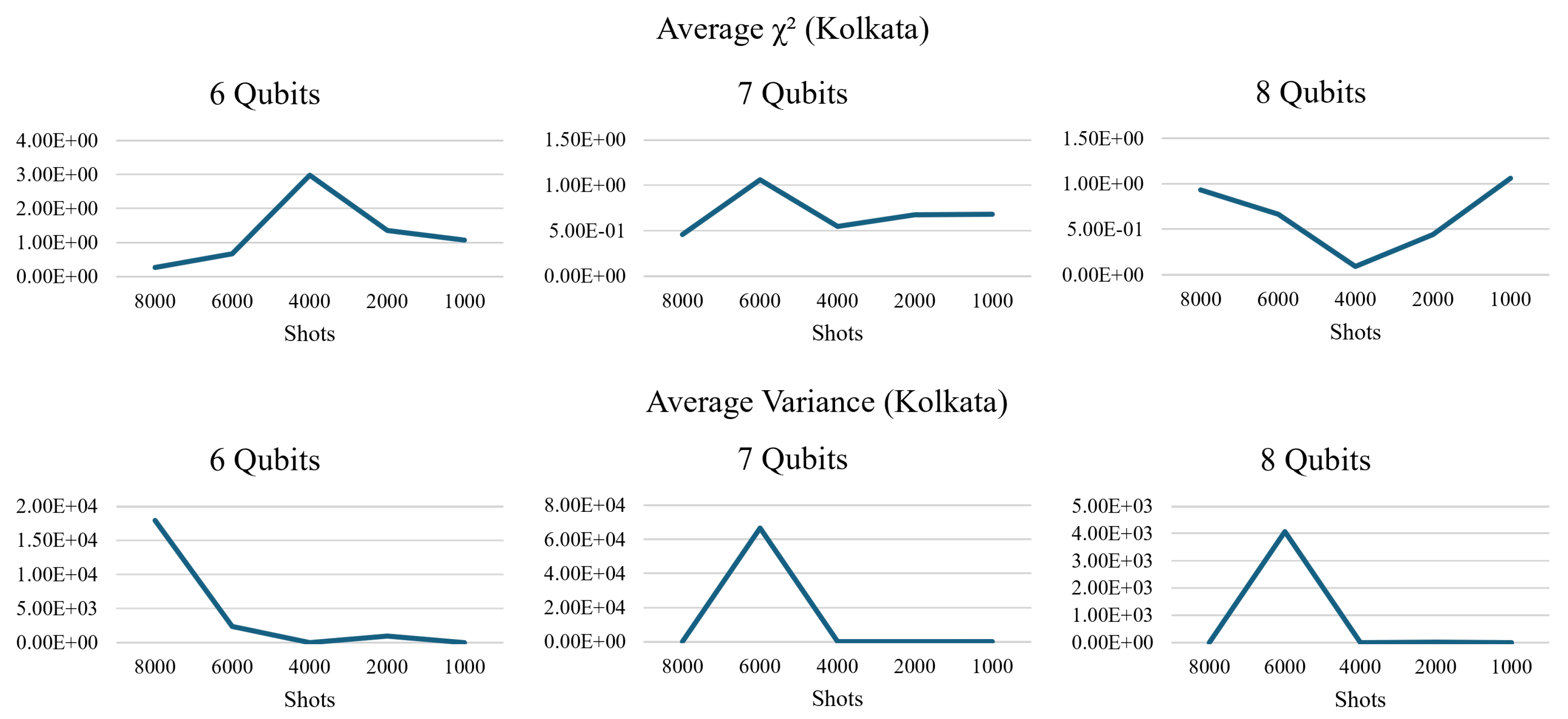
The results proved what we suspected from the B-SAT experiment, which is that the number of shots did affect the results in unusual ways. To be precise, the variance and fidelity did not peak at the lowest number of shots. As seen in Figure 20, the on the Kolkata quantum processor shows a predictable pattern by peaking at particular numbers of shots as the number of qubits increased. When the number of qubits is 5, the peaks at 2000 shots, and when the number of qubits is increased to 6, the peaks at 4000 shots. The pattern persists with the 7-qubit circuits where the peaks at 6000 shots. The 8-qubit circuit verified the previous pattern by the showing a spike in at the 8000 shot mark. It also showed signs of obeying the conceptual rules demonstrated in SubSection 2.4.1 by having a higher variance when the number of shots is set to the lowest setting in our experiments.
Kolkata also showed these spikes in variance, but they peaked in different number of shots than the as seen in Figure 20. The spike in variance seems to be set at 6000 shots when the number of qubits in the circuits is 7 and 8. Otherwise, the spike in variance followed the pattern when the number of qubits is 5.
The other quantum processor, Cairo, displayed a similar spike in variance and that repeats in the same number of shots and qubits(as seen in Figure 19). This would lead us to speculate that this occurrence is not tied to a single quantum processor. The spike is also present in the Hanoi quantum processor, albeit on the 4000 shots mark rather than the 2000 shots when running the 5-qubit circuit(shown in Figure 19).
Figure 19.
The number of shots across 5 different quantum processors seems to yield unusual results that do not follow the mathematical model(lower row). The drop in fidelity measured by the is also strangely tied to the number of qubits(upper row).
Figure 19.
The number of shots across 5 different quantum processors seems to yield unusual results that do not follow the mathematical model(lower row). The drop in fidelity measured by the is also strangely tied to the number of qubits(upper row).
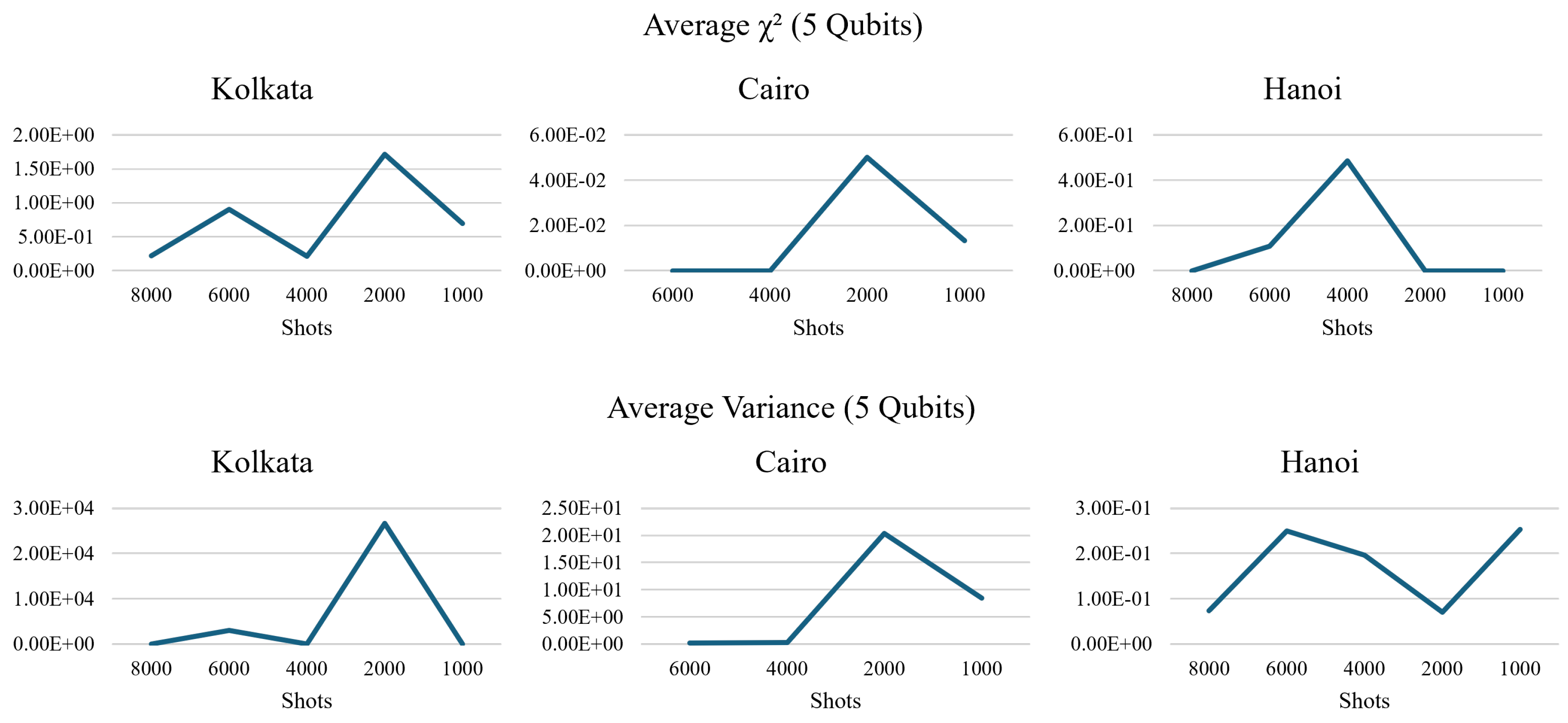
Figure 20.
The experiments executed with differing numbers of qubits on Kolkata show an atypical predictable fidelity loss spike shifting to the left with each increment to the number of qubits(upper row). The variance spikes at 8000 and 6000 shots on the 5+ qubit circuits(lower row).
Figure 20.
The experiments executed with differing numbers of qubits on Kolkata show an atypical predictable fidelity loss spike shifting to the left with each increment to the number of qubits(upper row). The variance spikes at 8000 and 6000 shots on the 5+ qubit circuits(lower row).
6. Conclusion
After performing numerous experiments, we have reached several key points regarding solving the B-SAT problem using quantum computing:
- The size, in terms of quantum volume and qubits, of a quantum processor is not an indicator of how well it performed in our B-SAT experiments. Quito, the quantum processor with fewer qubits , lower quantum volume, higher median readout and CNOT error rate than Lagos, yielded noticeably better results in the n=4 case.
- Increasing the number of shots did not result in a lower result variance, as it increased the variance in a certain higher number of shots. According to IBM, the cause of this issue is the firmware on their quantum processor. This hardware-firmware issue has affected numerous quantum experiments, not just our B-SAT experiment.
- The extra layer of qubit mapping almost always resulted in improved average results.
- A bigger circuit depth does not always imply worse results (at least not for an SAT circuit), as it sometimes gives us better results even when taking the random chance of success into account.
- The quantum processors experimented on performed adequately on the n=3 SAT and n=4 SAT circuits, but the results declined to noise level for the n=5 SAT and n=6 SAT.
Author Contributions
Conceptualization, A.B.; methodology, A.B.; software, A.B.; validation, A.B.; formal analysis, A.B.; investigation, A.B. and G.B.; resources, G.B. and P.F.; data curation, A.B.; writing—original draft preparation, A.B.; writing—review and editing, A.B. and G.B; visualization, A.B.; supervision, G.B.; project administration, P.F. All authors have read and agreed to the published version of the manuscript.
Funding
This research received no external funding
Institutional Review Board Statement
Not applicable
Informed Consent Statement
Not applicable
Acknowledgments
Special thanks to IBM for making it possible for us to use and experiment on their quantum processors. We are also thankful to John Streck for managing the quantum processor reservations that were used in this paper. Special thanks also go to the Kuwait Institute for Scientific Research for their financial help.
Conflicts of Interest
The authors declare no conflicts of interest.
Abbreviations
The following abbreviations are used in this manuscript:
| B-SAT | Boolean satisfiability problem |
| CNF | Conjunctive normal form |
| CNOT | Controlled not |
| EDA | Electronic design automation |
| EPC | Error per clifford |
| NISQ | Noisy intermediate-scale quantum era |
| QUBO | Quadratic unconstrained binary optimization |
References
- Zulehner, A.; Wille, R. Introducing Design Automation for Quantum Computing. Springer Nature, 2020.
- Turtletaub, I.; Li, G.; Ibrahim, M.; Franzon, P. Application of Quantum Machine Learning to VLSI Placement. Proceedings of the 2020 ACM/IEEE Workshop on Machine Learning for CAD, Nov. 2020. [CrossRef]
- Zalka, C. Grover’s quantum searching algorithm is optimal. Physical Review A 1999, 60, 2746–2751. [Google Scholar] [CrossRef]
- Cerf, N.J.; Grover, L.K.; Williams, C.P. Nested quantum search and NP-complete problems. arXiv [quant-ph], 1998.
- Tseitin, G. On the complexity of derivation in propositional calculus. Automation Of Reasoning: 2: Classical Papers On Computational Logic 1967–1970, 1983, pp. 466–483.
- Gabor, T.; Zielinski, S.; Feld, S.; Roch, C.; Seidel, C.; Neukart, F.; Galter, I.; Mauerer, W.; Linnhoff-Popien, C. Assessing solution quality of 3SAT on a quantum annealing platform. Quantum Technology And Optimization Problems: First International Workshop, QTOP 2019, Munich, Germany, March 18, 2019, Proceedings 1, 2019, pp. 23–35.
- Mézard, M.; Zecchina, R. Random k-satisfiability problem: From an analytic solution to an efficient algorithm. Physical Review E 2002, 66, 056126. [Google Scholar] [CrossRef] [PubMed]
- Qiskit-Community. Qiskit-Community/QGSS-2023: All things qiskit global summer school 2023: Theory to implementation - lecture notes, Labs and Solutions. Available online: https://github.com/qiskit-community/qgss-2023 (accessed on 23 August 2024).
- Marques-Silva, J.; Sakallah, K. Boolean satisfiability in electronic design automation. Proceedings of The 37th Annual Design Automation Conference, 2000, pp. 675–680.
- Cheng, S.; Tao, M. Quantum cooperative search algorithm for 3-SAT. Journal of Computer And System Sciences 2007, 73, 123–136. [Google Scholar] [CrossRef]
- Vinod, G.M.; Shaji, A. Finding solutions to the integer case constraint satisfiability problem using Grover’s algorithm. IEEE Transactions On Quantum Engineering 2021, 2, 1–13. [Google Scholar] [CrossRef]
- Fadillah, M.H.A.; Idrus, B.; Hasan, M.S.; Mohd, S. Impact of various IBM Quantum architectures with different properties on Grover’s algorithm. 2021 International Conference On Electrical Engineering And Informatics (ICEEI), 2021, pp. 1–6.
- D-Wave systems: The Practical Quantum Computing Company. Available online: https://www.dwavesys.com/.
- Kochenberger, G.; Hao, J.; Glover, F.; Lewis, M.; Lü, Z.; Wang, H.; Wang, Y. The unconstrained binary quadratic programming problem: A survey. Journal Of Combinatorial Optimization 2014, 28, 58–81. [Google Scholar] [CrossRef]
- Glover, F.; Kochenberger, G.; Hennig, R.; Du, Y. Quantum bridge analytics I: A tutorial on formulating and using QUBO models. Annals Of Operations Research, 2022, 314, 141–183. [Google Scholar] [CrossRef]
- Su, J.; Tu, T.; He, L. A quantum annealing approach for boolean satisfiability problem. Proceedings Of The 53rd Annual Design Automation Conference, 2016, pp. 1–6.
- Sahai, T.; Mishra, A.; Pasini, J.; Jha, S. Estimating the density of states of Boolean satisfiability problems on classical and quantum computing platforms. Proceedings Of The AAAI Conference On Artificial Intelligence 2020, 34, 1627–1635. [Google Scholar] [CrossRef]
- Ramos-Calderer, S.; Bravo-Prieto, C.; Lin, R.; Bellini, E.; Manzano, M.; Aaraj, N.; Latorre, J. Solving systems of Boolean multivariate equations with quantum annealing. Physical Review Research 2022, 4, 013096. [Google Scholar] [CrossRef]
- Nation, P.; Treinish, M. Suppressing Quantum Circuit Errors Due to System Variability. PRX Quantum 2023, 4, 010327. [Google Scholar] [CrossRef]
- Qiskit. “Randomized benchmarking.” Randomized Benchmarking-Qiskit Experiments 0.5.4 Documentation. Available online: https://qiskit.org/ecosystem/experiments/manuals/verification/randomized_benchmarking.html (accessed on 7 November 2023).
Figure 1.
A CNF circuit represented in digital logic form and its different stages are outlined
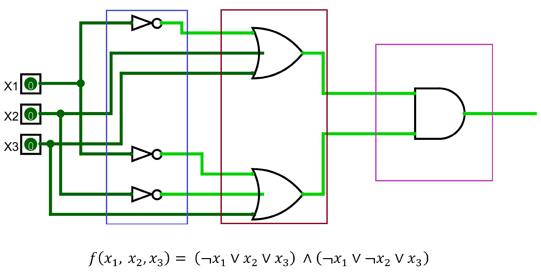
Figure 2.
In this example, the CNF circuit would be: . It should be noted that this example has only 1 distinct solution.
Figure 2.
In this example, the CNF circuit would be: . It should be noted that this example has only 1 distinct solution.
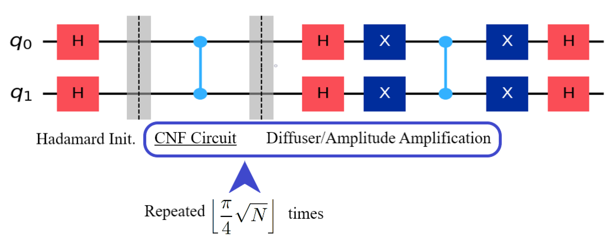
Figure 3.
While these two quantum circuits have almost double the amount of quantum gates, they have identical quantum circuit depth. Parallel operations do not accumulate.
Figure 3.
While these two quantum circuits have almost double the amount of quantum gates, they have identical quantum circuit depth. Parallel operations do not accumulate.
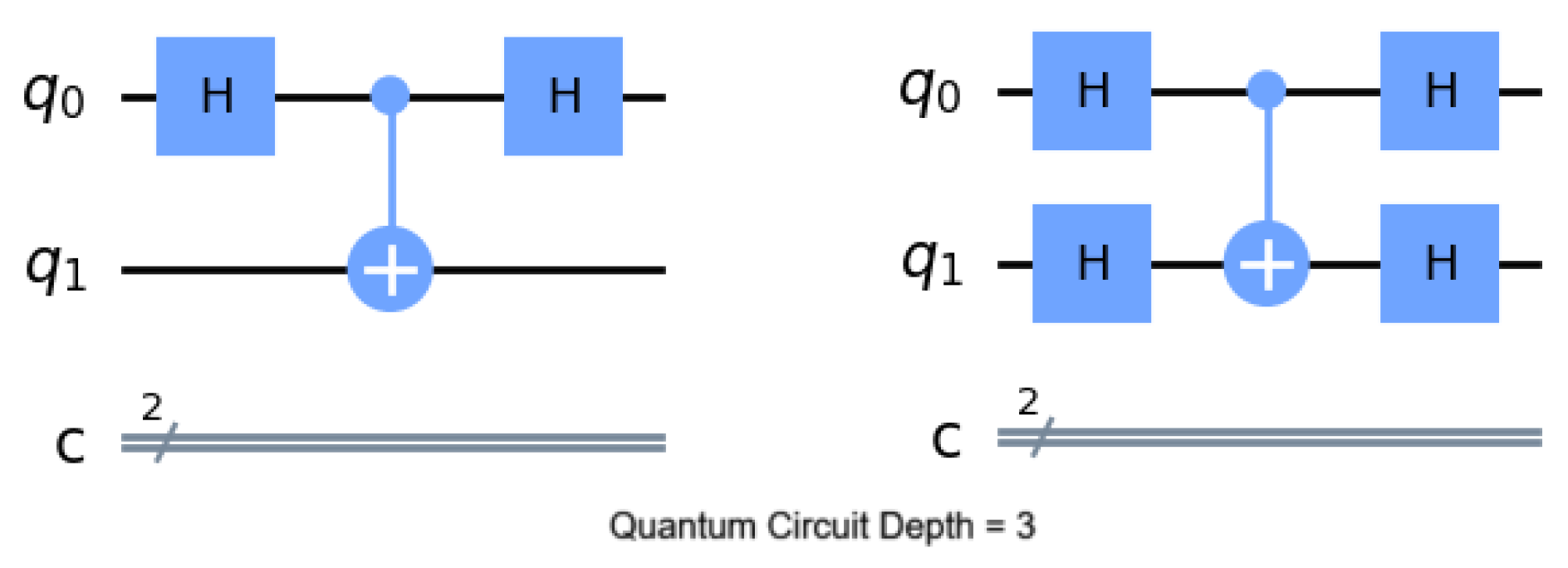
Figure 4.
Variance of Random Classical Variable Vs. Probability to Measure 1. The probability of yielding outlier mean measurements decreases as the number of shots is increased, hence this should be an indicator that the variance should decrease as the number of shots is increased.
Figure 4.
Variance of Random Classical Variable Vs. Probability to Measure 1. The probability of yielding outlier mean measurements decreases as the number of shots is increased, hence this should be an indicator that the variance should decrease as the number of shots is increased.

Figure 5.
A brief summarization of the experimental procedure
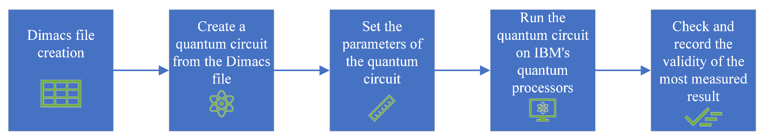
Figure 6.
This is a figure that summarizes our experimental procedure. The black arrows are to be repeated 3 times per cycle, while the olive-colored lines are performed once per cycle.
Figure 6.
This is a figure that summarizes our experimental procedure. The black arrows are to be repeated 3 times per cycle, while the olive-colored lines are performed once per cycle.
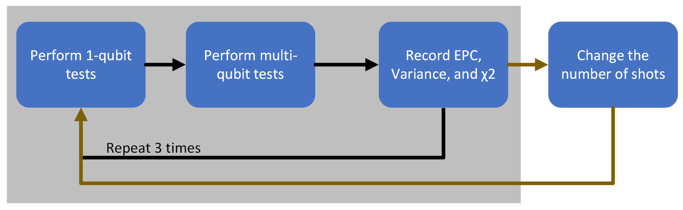
Figure 7.
The n=3 SAT results on Quito gave us almost perfect answers with few outliers here and there
Figure 7.
The n=3 SAT results on Quito gave us almost perfect answers with few outliers here and there

Figure 8.
Circuit depth seems tied to more positive results with the unmapped n=3 B-SAT.
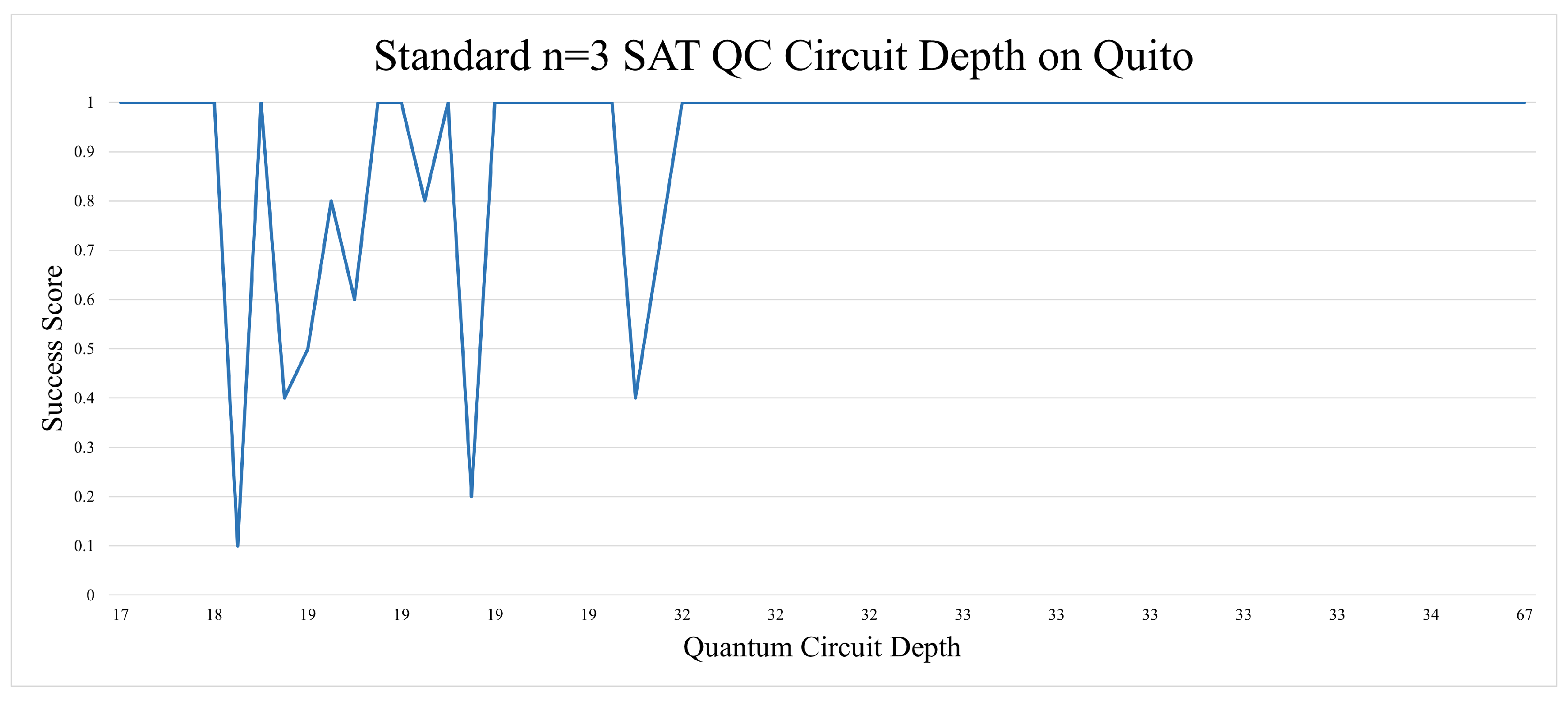
Figure 9.
Qubit mapping did not improve the n=3 SAT results by much.
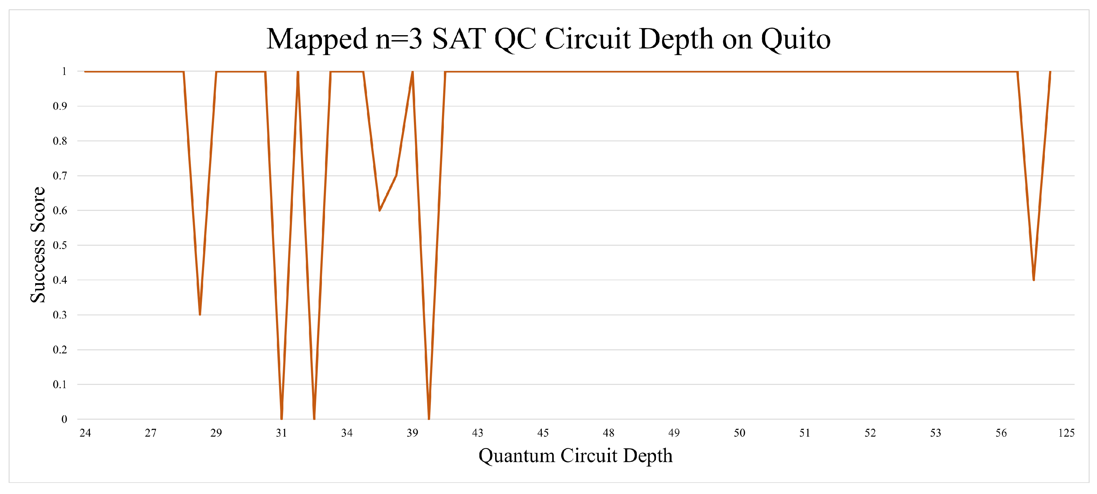
Figure 10.
Increasing the n to 4 marks a noticeable decline in the success score, but the results some improvement when using qubit mapping and increasing the number of shots per execution
Figure 10.
Increasing the n to 4 marks a noticeable decline in the success score, but the results some improvement when using qubit mapping and increasing the number of shots per execution
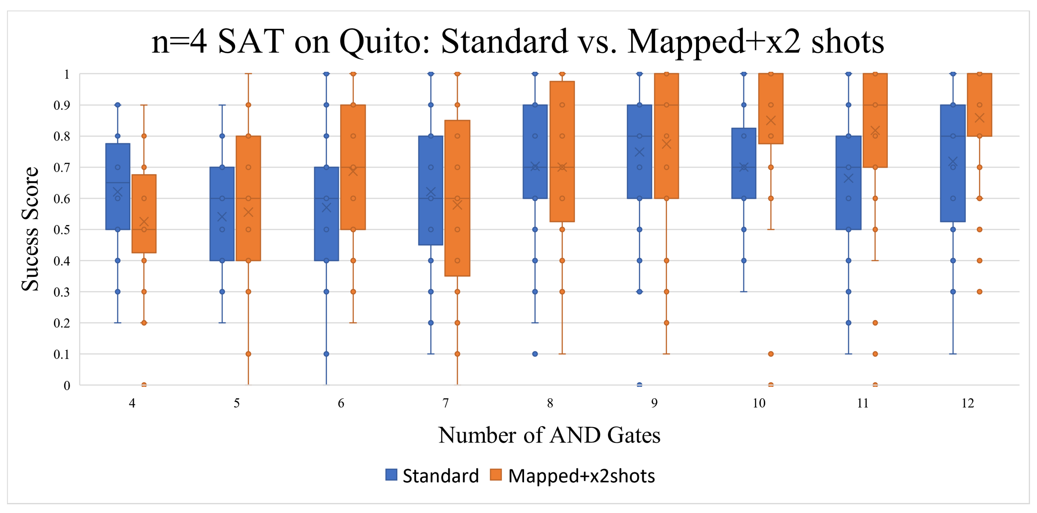
Figure 11.
Either/or doubling the number of shots and using qubit mapping has resulted in an aggravated Success Score
Figure 11.
Either/or doubling the number of shots and using qubit mapping has resulted in an aggravated Success Score
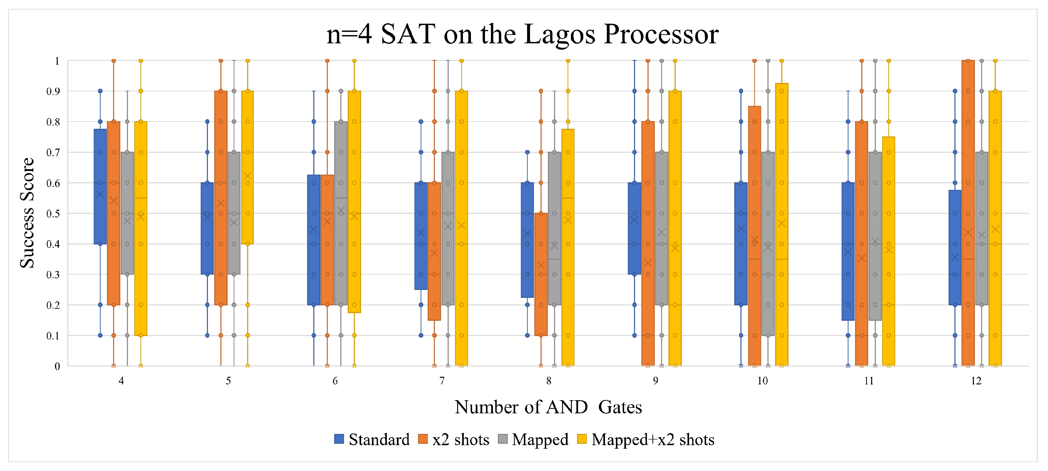
Figure 12.
The dotted blue line marks a polynomial aggregation of the experimental results.
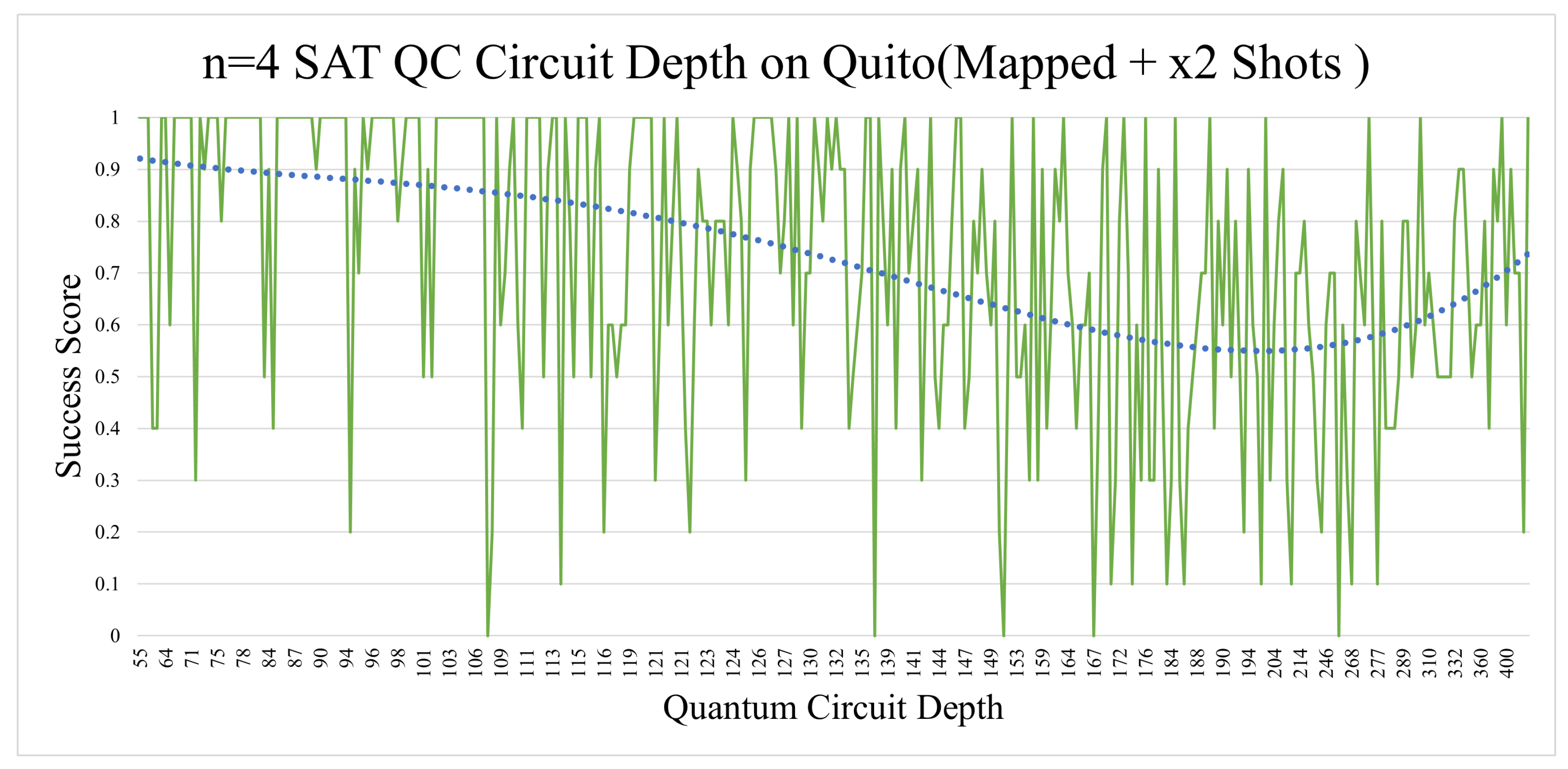
Figure 13.
There was no noticeable pattern with the depth aspect of the n=4 SAT runs on Lagos.
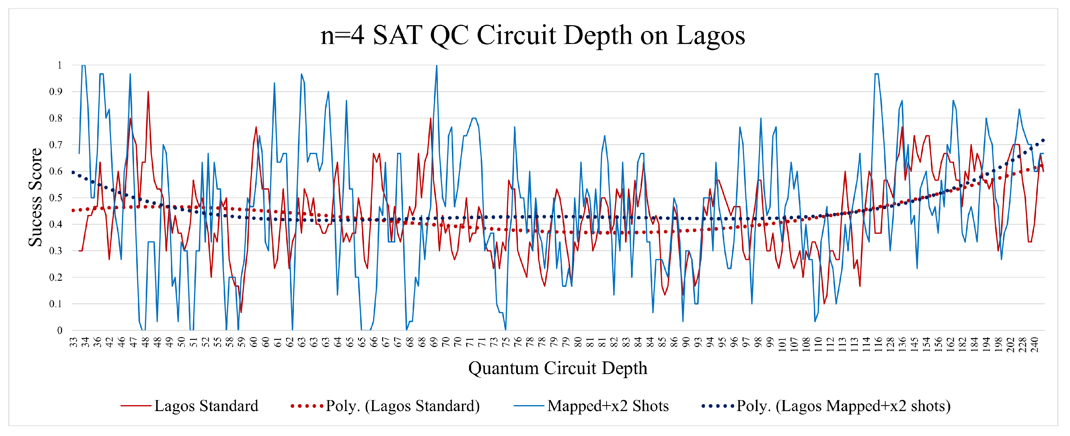
Figure 14.
Both Quito and Lagos seem to have produced similar results, which would be interpreted as noise when factoring in the random chance of success
Figure 14.
Both Quito and Lagos seem to have produced similar results, which would be interpreted as noise when factoring in the random chance of success
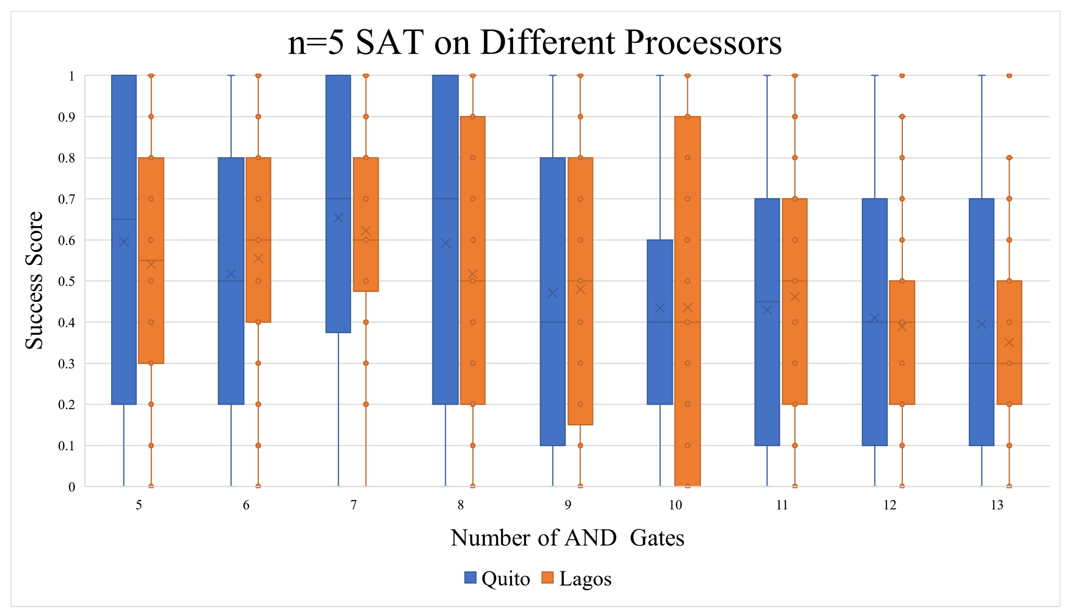
Figure 15.
In this case, the n=5 SAT experiments indicate that high circuit depth is caused by a higher number of OR gates, which results in a higher probability of random success
Figure 15.
In this case, the n=5 SAT experiments indicate that high circuit depth is caused by a higher number of OR gates, which results in a higher probability of random success

Figure 16.
As the number of AND gates increases, the results drop to just noise level integrity
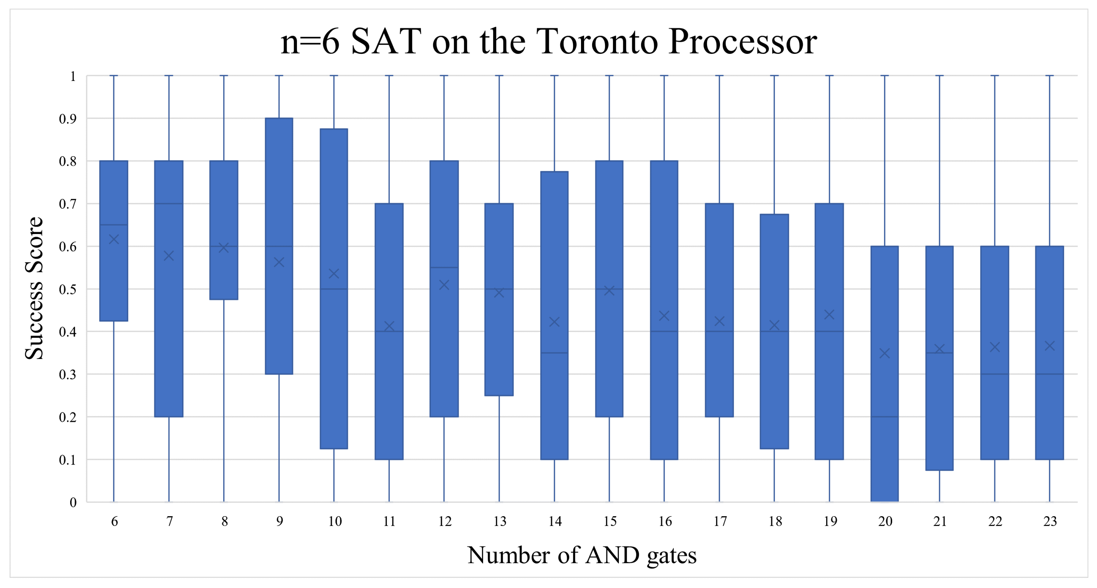
Figure 17.
The correlation of a higher circuit depth and success score could be caused by the circuits having a higher proportion of OR to AND gates
Figure 17.
The correlation of a higher circuit depth and success score could be caused by the circuits having a higher proportion of OR to AND gates
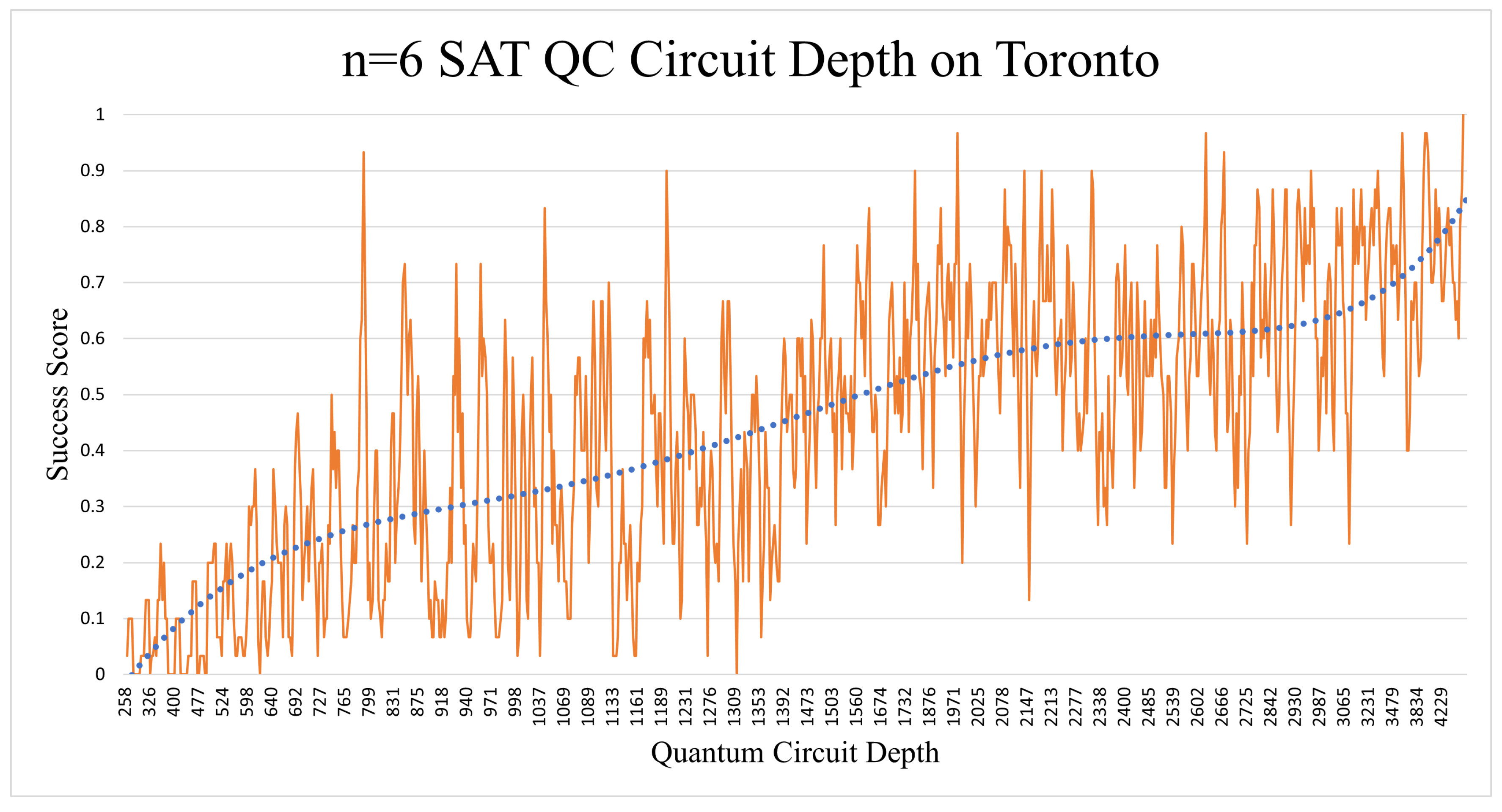
Figure 18.
The ratio of OR:AND gates is what decides how big the span of satisfiable solutions
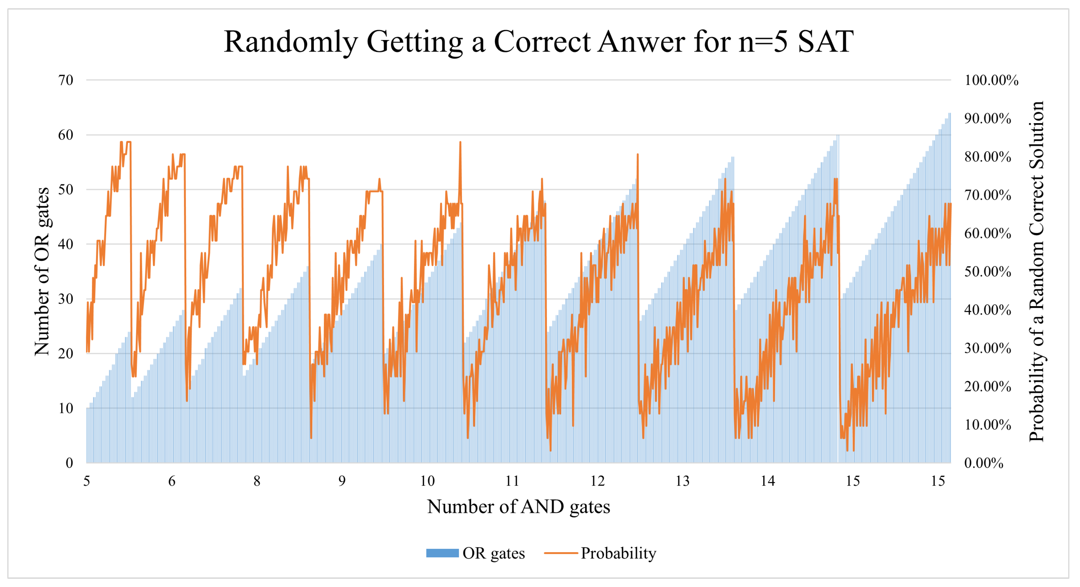
Table 1.
An outline of the classical and quantum expectation value squared.
| Classical | Quantum |
Table 3.
Number of dimacs Files Generated per Configuration
| SAT Configuration | Number of dimacs Files Generated |
|---|---|
| n=3 | 64 files |
| n=4 | 325 files |
| n=5 | 709 files |
| n=6 | 880 files |
Table 6.
Statistical Comparison Between the Experimental Results vs. Probabilistic Chance of Random Success
Table 6.
Statistical Comparison Between the Experimental Results vs. Probabilistic Chance of Random Success
| Quantum Processor | Probablistic |
|---|---|
| n=3 SAT on Quito | n=3 SAT |
| Average: 93% | Average: 39% |
| Median: 100% | Median: 43% |
| n=3 SAT Correlation: -0.5311 | |
| n=4 SAT on Quito (Mapped+x2 Shots) | n=4 SAT |
| Average: 73% | Average: 42% |
| Median: 80% | Median: 40% |
| n=4 SAT Correlation: -0.4132 | |
| n=5 SAT on Quito (1 Iteration) | n=5 SAT |
| Average: 50% | Average: 46% |
| Median: 50% | Median: 48% |
| n=5 SAT Correlation: 0.4852 | |
| n=6 SAT on Toronto | n=6 SAT |
| Average: 44% | Average: 44% |
| Median: 40% | Median: 45% |
| n=6 SAT Correlation: 0.6176 | |
Disclaimer/Publisher’s Note: The statements, opinions and data contained in all publications are solely those of the individual author(s) and contributor(s) and not of MDPI and/or the editor(s). MDPI and/or the editor(s) disclaim responsibility for any injury to people or property resulting from any ideas, methods, instructions or products referred to in the content. |
© 2024 by the authors. Licensee MDPI, Basel, Switzerland. This article is an open access article distributed under the terms and conditions of the Creative Commons Attribution (CC BY) license (http://creativecommons.org/licenses/by/4.0/).
Copyright: This open access article is published under a Creative Commons CC BY 4.0 license, which permit the free download, distribution, and reuse, provided that the author and preprint are cited in any reuse.


