Submitted:
30 August 2025
Posted:
02 September 2025
You are already at the latest version
Abstract
Personalised modelling has become dominant in personalised medicine and precision health. It creates a computational model for an individual based on large data repositories of existing personalised data, aiming to achieve the best possible personal diagnosis or prognosis and derive an informative explanation for it. Current methods are still working on a single data modality or treating all modalities with the same method. The proposed method, SAIN (Search-And-INfer), offers better results and an informative explanation for classification multimodal object (sample) using a database of similar multimodal objects. The method is based on different distance measures suitable for each data modality and introduces a new formula to rank each sample and then use these ranks for a probabilistic inference. The paper describes SAIN and applies it to two types of multimodal data, cardiovascular diagnosis and EEG time series, modelled by integrating modalities, such as numbers, categories, images, and time series, and using a software implementation of SAIN. search in multimodal data; inference in multimodal data; personalised modelling; precision health.
Keywords:
search in multimodal data
; inference in multimodal data
; personalised modelling
; precision health.
1. Introduction
Multimodal data has been gathered at a personalised level in large quantities, worldwide, for many applications, such as neuro-imaging analysis, personalised health diagnosis and prognosis, environmental modelling, and financial modelling, to mention only a few of them. Still, there are no efficient methods to integrate various multimodal data for a new subject and derive a more accurate and explainable diagnosis or prognosis based on existing multimodal data of many other subjects. The goal of this paper is to create such a method.
There are three main approaches to multimodal data integration in machine learning, explored so far [1]:
1. Early integration, where a common vector represents all modalities used for training a model and for its recall. This approach has been used for integrating time series and textual information [2,3], for image integration [4], and for the integration of clinical, social, and cognitive data modalities to predict psychosis in young adults [5]. While the method in [4] is based on deep, feedforward neural networks, the methods in [2,5] use a brain-inspired spiking neural network architecture NeuCube [6].
2. Late integration, where a model is created and trained for each of the modalities of data, and the results from all models are integrated to calculate the output. This approach has been demonstrated in [1] on integrating clinical, genetic, cognitive, and social data for medical prognosis.
3. Hybrid, early, late, and intermediate integration of data modalities, where the two approaches above are combined [1].
The proposed SAIN method in this paper is designed for early integration of data modalities, where specific encoding and distance metrics are suggested for different types of data, along with novel algorithms for search in a multimodal database and inference. These search and inference algorithms are related to building a personalised model for individual outcome assessment and its explanation.
Personalised modelling is concerned with the creation of an individual model for a new personal (individual) record of data X, using an already existing repository D of many other personal records for which the outcomes are known, to assess the outcome of the new record X [7]. Methods for personalised modelling have been developed to work mainly on a single modality of data [8,9]. These methods have been applied in many applications and constitute the state-of-the-art in the field (e.g. [1,9,10,11,12,13]). In [9,14], a personalised modelling is proposed based on static and temporal modalities of data, which are used to train a spiking neural network model.
The enormous growth of personal multimodal data worldwide demands more advanced methods for personal modelling with the use of multimodal data. This paper offers such a method, called SAIN, where the specificity of each data modality is considered and new algorithms are proposed for the encoding of multimodal data, for search in a multimodal data repository, and for multimodal inference, along with its explanation and visualisation. In contrast with the statistical solutions used in [15,16,17], we adopt a probabilistic framework that gives more precise evaluations of probabilities of outcomes for an individual.
2. Mathematical Description
In this section, we present the mathematical method. In detail, we start with the database coding and a class of distances (metrics) to be used in this article, followed by the list of tasks (problems) and their solutions. Detailed examples illustrate the solutions. Detailed solutions to three critical problems, survival analysis, heart disease diagnosis, and time series classification, are presented in detail and illustrated with numerical examples.
2.1. Database
We will work with the multidimensional data described as follows:
- objects (samples) ,
- each object () is defined by criteria (variables) with values in linearly ordered domains with and ; if some value (, ) is either missing or uncertain, then its value is recorded as ∞,
- weights in with , where each () quantifies the importance of the criterion ; if for all , then all criteria are equally important; a criterion is ignore if .
Data of independent variables are organised as in (Table 1):
2.2. Distance Metrics
A distance metric on a space X is a positive real-valued function satisfying the following three conditions for all : a) if and only if , b) , c) .
The multicriteria metrics [18,19] (used in multicriteria recommendation systems [20]) presented in this part can be used on a variety of domains : they can be sets of logical values, rational numbers, percentages, digitally codified images, sounds, videos, and many others. We use a bounded distributive complemented lattice to describe uniformly the domains . We rank all objects according to their aggregated distance to a new one; based on that, we calculate probabilities of the new object belonging to different classes, represented in the object repository.
Here is a list with illustrative, but far from exhaustive, examples of domains :
- Logical Boolean domain: , where .
- Logical non-Boolean domain: , where and .
- Numerical domain with natural values: , where .
- Numerical domain with rational values: , where .
- Binary code: , where the domain consists of all binary strings of length n, and for all , , ,
In the lattice we introduce, following [18], the metric:
for . This metric d can be extended to as follows:
where .
The metrics on , , can be extended to , i.e. to n-dimensional vectors, as follows:
where , .
In what follows, we write d for when the meaning is clear from the context.
2.3. Tasks Specification
Data organised as in Table 2, Table 3, and Table 4 consists of independent objects augmented with a column of labels, the weights of criteria, and a new unlabelled object, respectively.
Additional information associated with data in Table 2 may include the range of each criterion and the associated specific distance, e.g. the Euclidean distance for real numbers and the distance d for binary strings or strings over a non-binary alphabet (e.g. for images or colours).
We consider the following tasks:
- Task 1:
-
Calculate the distance (or similarity metric) between the new object and each object in Table 2.If the distance corresponding to is , then
- Task 2:
- Given a threshold , calculate all objects at a distance at most to x.
- Task 3:
- Calculate the probability of a new object belonging to a labelled class (e.g. low risk vs. high risk) using a threshold and Table 2.
- Task 4:
- Rank the criteria in Table 2 and calculate the marker or markers criterion/criteria that are the most important/ones.
- Task 5:
- Assign alternative weights to criteria.
- Task 6:
- Test the data accuracy and method for Task 4.
2.4. Tasks Solutions
For Task 2, given a threshold , we calculate all objects in Table 2 at a distance at most to x, that is, the objects which are -similar to x:
and its complement .
For Task 3 we calculate the probability that x is in class label , which is the ratio of the number of objects in with the label to the size of the cluster :
where means the number of elements in the set .
For Task 4, we work with Table 2. Recall that for each criterion we have a domain augmented with information “high" or “low," indicating whether higher or lower values are desirable. Based on this information, we can construct a hypothetical object (see Table 5) which has the most desirable values for each criterion: one could see this object as an “exemplar" one.
Sometimes, criteria are interrelated or correlated. This means that in some cases, there is no unique “exemplar object", but a couple of them have to be studied in ranking the importance of criteria.
For example, fix an “exemplar object" .
- Compute the distances between each object in Table 2 and , so obtain a vector with n non-negative real components .
- For each , compute the distances taking into consideration all criteria in Table 2 except: obtain the vector .
- Compute the distances between , using the formulaand sort them in increasing order. The criterion is a marker if , for every .
We repeat this procedure for each “exemplar object" and study possible variations.
For Task 5, normalise the distances and use these values to construct the weights , .
2.5. An Example
We illustrate the above tasks with an example of a labelled database in (see Table 6) and a new object (see Table 7), all having the following seven characteristics (the last column has the label classes 1 and 2):
: real number , e.g. age, weight, BMI etc.;
: Boolean value , e.g. gender;
: integer number , e.g. gene expression;
: categorical {small, med, large }, e.g. size of tumour, body size, keywords;
: colour {red, yellow, white, black}, e.g. colour of a spot on the body, on the heart;
: spike sequence of e.g. encoded EEG, ECG;
: black and white image, e.g. MRI, face image.
In this fictitious example, for simplicity, we didn’t use weights.
Then, we normalise the data in Table 8 and Table 9 – the entries in the first, third, and fourth columns have been divided by 100, 10,000, and 2, respectively. The entries in the last three columns have been transformed into reals in the unit interval, and the column of labels has been removed. In this way, we have obtained Table 10 and Table 11.
Then, we choose an appropriate distance according to each criterion. In this example, we used the Euclidean distance for all criteria (see Table 12 and Table 13).
We can compute and, accordingly, the probability that x would be labelled in class 1 or class 2.
If , then so the probability that x is in class 1 is 2/7 and the probability that x is in class 2 is 5/7. If , then its closest cluster is , so the probability that x is in class 1 is 1/3 and the probability that x is in class 2 is 2/3.
which induces a ranking of the objects in the Table 8: .
2.6. Complexity Estimation of the SAIN Method
The proposed method to compute the similarity between a new object and N objects in a data repository is linear in N, so very fast.
3. Survival Analysis in SAIN
Medical survival analysis evaluates the time until an event of interest occurs, like death or disease recurrence, in a group of patients. This analysis is often used to compare treatment outcomes or predict prognosis. In contrast with the statistical solutions used in [15,16,17], we adopt a probabilistic framework that gives more precise evaluations of probabilities.
3.1. Data and Tasks
We are given the following data:
- Table 17 in which the first column lists the patients treated for the same disease with the same method under strict conditions, and the last column records the times till the patients’ deaths.
- Table 18, which includes the record of the new patient p.
- A threshold which defines the acceptable similarity between p and the relevant ’s in the Survival database (i.e. ).
We consider the following tasks:
Task 1: What is the life expectancy of p?
Task 2: What is the probability that the life expectancy of p is greater than or equal to a given T?
3.2. Tasks Solutions
Using a standard method of survival analysis
-
For Task 1,
- (a)
- Compute the set of patients that are similar up to to p:
- (b)
- Using , compute the probability that p will survive the time :
- (c)
- Compute the life expectancy of p using the formula:
- For Task 2, calculate the probability that the life expectancy of p is at least time T:
3.3. An Example
We illustrate the above tasks with an example of a database in which columns 2–8 record patients’ medical test results, and the last column records time to death (see Table 19) and a new patient (see Table 20):
The distance for column 4 is and . For example, . For all other columns, the distance is . Finally, the total distance is the sum of individual distances (7 terms), with the results in Table 21.
The results for Task 1, (a), (b), and (c) are listed below:
-
For , , that is the entire database. Then
- (a)
- ,
- (b)
- i.
- ,
- ii.
- ,
- iii.
- ,
- iv.
- ,
- v.
- ,
- vi.
- ,
- vii.
- ,
- viii.
- .
- (c)
- i.
- ,
- ii.
- ,
- iii.
- ,
- iv.
- ,
- v.
- ,
- vi.
- ,
- vii.
- ,
- viii.
- ,
We can calculate other probabilities, for example, . -
For , . Then
- (a)
- ,
- (b)
- i.
- ,
- ii.
- ,
- iii.
- ,
- iv.
- ,
- v.
- ,
- (c)
- i.
- ,
- ii.
- ,
- iii.
- ,
- iv.
- ,
- v.
- .
Similarly, we can calculate the probabilities , .
In contrast with the statistical solutions used in [14,15,16], we adopted a probabilistic framework that gives more precise evaluations of probabilities. The SAIN algorithms also include some statistically established methods, such as the t-test, for ranking variables before applying the inference method.
4. SAIN: A Modular Diagram and Functional Information Flow
The SAIN framework consists of the following modules (Figure 1):
- Multimodal data of a new object X.
- An existing repository D of multimodal data of many objects, labelled with their outcome.
- A module of algorithms for searching in the database D and based on the distance between X and each object in D.
- Defining a subset from D, so that X is closer to the objects in based on a given threshold.
- A module of algorithms for building a model in .
-
An inference algorithm to derive the output for X from the model and to visualise it for explanation purposes. Figure 1 gives a modular view of the SAIN framework and Figure 2 shows the information processing flow:
- (a)
- Encoding the multimodal data of X and D. -
- (b)
- Choosing a distance matrix and similarity search in the data set D.
- (c)
- Calculating the aggregated difference between the new data vector X and the closest vectors in .
- (d)
- Creating a model in .
- (e)
- Applying inference by calculating the for each class (or output value), using the wwkNN method in [5].
- (f)
- Reporting and visualisation of results of the individual model Mx. This is illustrated in Figure 3.
The inference method is based on the wwkNN (weighted variables, weighted samples k-nearest neighbour) proposed by Kasabov [7]. This method first ranks the impact of the variables (multimodal ones) to estimate their weights/impact towards the output using a t-test; then, it measures the distance between the new object X and the ones in the database and weighs it. For each class , the higher a variable is ranked, the closer the samples/objects belong to class . to X, the higher the calculated value of is. The new object X is classified in class if is the highest among all values In Figure 1 and Figure 2, we present the modular diagram and the functional information flow of SAIN.
Figure 1.
A modular diagram of the proposed SAIN computational framework
Figure 2.
A flow of data and information processing in the SAIN computational framework
Figure 3.
An example of visualisation of a personalised SAIN model. The closest four samples (out of 6) to the new object (star) are from class 1 (in red) using the top three informative variables. Each sample is a multimodal one, and the top 3 variables can be of different modalities
Figure 3.
An example of visualisation of a personalised SAIN model. The closest four samples (out of 6) to the new object (star) are from class 1 (in red) using the top three informative variables. Each sample is a multimodal one, and the top 3 variables can be of different modalities
5. Case Studies for Medical Diagnosis and Prognosis
We present three case studies in which we applied SAIN.
5.1. Heart Disease Diagnosis
We worked with the well-known Cleveland dataset, which contains multiple data types [21]. The UCI Heart Disease data set includes 76 attributes. As in most articles, the attributes in our experiment data were restricted to 14, see Table 22.
The problem is a binary classification of whether the patient has or does not have heart disease.
First, we selected suitable distance metrics and weights to classify the attributes. For binary objects, the distance metric is simply whether they are equal; for non-binary discrete objects such as resting electrocardiographic results, the appropriate distance measure is not obvious and should be informed by an expert. We give electrocardiographic results 0 for normal, 1 for having ST-T wave abnormality, and 2 for showing probable or definite left ventricular hypertrophy following Estes’ criteria.
Many studies with the Cleveland dataset have been tested with different machine learning techniques. For example, [21] lists different algorithms and performances ranging from 47% to 80% accuracy. SAIN achieved an 82% accuracy score. Why SAIN? The search is fast, uses appropriate distances chosen by a medical expert, and provides explainability at a personal level, including probabilities. It offers different scenarios for modelling by experimenting with different sets of features, parameters, and preferred outcome visualizations.
The SAIN experiment used binary and numerical representation for each variable as described. We have used the same data representation (recommended by medical experts) as in the original paper [21]. The accuracy of the SAIN experiment was 82%, the same accuracy as in [6], which used classical machine learning. In addition, SAIN allows visualising each personalised model as shown in the examples in Figure 3 and Figure 8.
5.2. Time Series Classification
The proposed SAIN framework can incorporate time series data, as another modality, in addition to other modalities of data for a person, making a joint multimodal personal vector. A time series data is encoded into binary vector by using spike encoding algorithms [6], where if there is a positive change from one discrete time point to the next one in the time series, there will be a positive spike( encoded as 1); a negative change will result in a negative spike (-1) and no change will result in 0 value. This is illustrated on a hypothetical time series in Figure 4. This approach applies to any time series raw data, at any time scales, and here we show just two hypothetical examples of brain EEG data (Figure 5) and cardio data (Figure 6).
Many data sets for classifying outcomes of events consist of multiple time series. Each variable in a time series may depend on other variables that change in time. The proposed model can deal with this problem by encoding time series (signal) into binary vectors, which can be processed for classification in the SAIN framework. The variables for this data set are 14 channels of temporal EEG data, located at places of interest on the human scalp.
The signals measured over the same period are the EEG channels, fMRI voxels, ECG electrodes, seismic sensory signals, financial time series, gene expressions, voice, and music frequency bands [11]. Even when the variable (signal) measurements are independent, the signals may impact each other as they represent the same object/person at the same time period. The number N of these signals can vary from just a few for a short time window T (Figure 4) to hundreds and thousands when the time varies from a few milliseconds to minutes, hours, days, etc.
Next, we present a simple example of how this search can be computed for a new record X consisting of only three variables/signals (e.g., EEG channels, ECG electrodes) over a short period of 5 time moments and the database D consisting of only six such records, which are labelled by outcome labels 1,2,3 (e.g., diagnosis, prognosis).
In addition to the record X, a weight vector is supplied with the weighted importance of the signals at different time points, e.g. , meaning that the most important and informative part of the measurements is at time point 3.
The new record (signal, EEG channel 1) 0, 1, 1, 1, -1 (signal, EEG channel 2) 1, 1, -1, -1, 0 (signal, EEG channel 3),
The database contains records where (see Table 23):
The new record X of EEG-signals will be classified in class 1 as it is closest according to the Euclidean distance, class 1 data samples and .
5.3. Predicting Longevity in Cardiac Patients
We utilised a data set [22] in which we applied a binary classification on whether the patient had an event (e.g., death) and further to those that had an event, whether this would occur in the near future (within the next 180 days, e.g., approximately six months). The data set contained a set of 150 variables and an outcome, with 295 patients in the first data set and 49 in the second. The data included a mix of variables that could be grouped as follows:
- demographics, risk factors, disease states, medication and deprivation scores,
- echocardiography, cardiac ultrasound measurements,
- advanced ECG measurements,
The other data includes the days until the event occurred and the censor date for the Cox proportional hazard monitoring.
The objectives are to predict an arrhythmic event or death.
Before running the algorithm, the data was normalised, and to account for the data being unbalanced, we utilised the SMOTE data balancing method [11] each time we left one out (ensuring that we did not SMOTE when the true data point was part of the data set). For the event classification data set, the model achieved an accuracy of 79%. This is broken down into classifying no event (198/247, 80%) and an event with (36/49, 73%) accuracy. It is worth noting that the confidence of each individual could be explored with a sample of the confidence for classification in Figure 7.
For the second experiment, we normalised the dataset and removed any columns with unknown values. We then applied a genetic algorithm to find the set of features to use for classification. We found a set of 34 variables which would provide an accuracy of with (34/34) for class 0 and (6/15) for class 1. Alternatively, if we apply SMOTE and focus more on the accuracy of class 1, we obtain accuracy, however, more evenly distributed with (24/34) for class zero and (10/15) for class 1.
Experiment one, in which we used a non-balanced complete data set, showed satisfactory results of 80% for class 0 (no event) and 73% for class 1 (event). This demonstrates the ability of the SAIN method to work with imbalanced data. It also shows the superiority of utilising the missing values rather than removing them in experiment two. Furthermore, the selection of variables with a genetic algorithm also showed improvement. The genetic algorithm, included in the SAIN software, can also help select biomarker variables in other cases (See Figure 8).
Figure 8.
An individual model of survival showing the closest neighbouring samples in the top 3 ranked variables
Figure 8.
An individual model of survival showing the closest neighbouring samples in the top 3 ranked variables
6. Data and Software Availability
The data has been obtained from the UCI Cleveland from https://archive.ics.uci.edu/dataset/45/heart+disease; the EEG data is available from https://github.com/KEDRI-AUT/NeuCube-Py/tree/master/example_data. Access to the software is available on request.
7. Conclusions
The paper presents a new search and inference method, called SAIN, for multi-modal data integration and personalised model creation based on these multi-modal data. The model not only evaluates the outcome for a person more accurately than traditional machine learning methods using a single modality of data, but it also explains the proposed solution in terms of probability and visual explanation.
In its current form, the paper is more directed towards revealing a new methodology and algorithms than real full-scale medical applications. However, we have illustrated the methods using hypothetical and real case health and medical data sets. Further utilisation of the proposed framework is currently being developed for large-scale biomedical data.
The proposed new method offers new functionality and features for personalised search and model creation in multimodal data, some of which are listed below:
- The method is suitable for multimodal data searches in heterogeneous data sets, e.g., numbers, text, images, sound, categorical data;
- It is suitable for personalised model creation to classify or predict specific outcomes based on multimodal and heterogeneous data.
- It uses a similarity measure based on multicriteria metrics. In this way, inaccurate measurement of similarity on a large number of heterogeneous variables is avoided.
- Its search is fast even on large data sets and includes advanced personalised searches with multiple parameters and features;
- It facilitates multiple solutions with corresponding probabilities;
- It is suitable for unsupervised clustering in multimodal heterogeneous data.
The proposed method is implemented as a computer system and applied to several case studies to illustrate its advantages and applicability. The SAIN method described in Section 4 was implemented as a software system.
In conclusion, integrating all possible data modalities for a single subject to predict/classify the object’s state in relation to existing ones is an open problem in data science. While the creation of personalised models based on a single modality data [23] and clustering of single modality data into a single cluster [24] have been successfully developed, the theory, framework and algorithms, proposed in this paper, are the first to integrate all data modalities for a single subject together into a single vector-based representation and to make an inference based on it. For the first time, time series, such as EEG and ECG data, are included in this unified representation, after suitable encoding. In this respect, spike encoding of time series is used, integrating statistical and brain-inspired information representation. The human brain integrates sensory data modalities into its spatio-temporal structure, and brain-inspired models using spike information representation have already been developed for learning [6,11,25] and for explanation of the learned patterns [26]. However, brain-inspired computers are still in their early stage of development [11], and even if they are developed, they may not be able to integrate all possible modalities of data into one brain-inspired mode. This paper offers a solution to the problem of multimodal personalised data integration and inference, six novel features characterise that: (1) it includes all possible modalities of data; (2) it can be implemented on any conventional computer platforms; (3) it takes into account the differences across modalities of data through offering different distance measures; (4) it offers a new way of ranking existing multimodal objects in order of similarity to a new multimodal object and uses that for building multiple neighbourhood clusters; (5) it offers a probability based inference with the use of the different similarity clusters; (6) it explains the inferred results, both in terms of probabilities and visual representation. The proposed original method here is planned to be applied to large-scale multimodal data for biomedical and health applications in the future.
The proposed method is implemented as a computer system and applied to several case studies to illustrate its advantages and applicability. The SAIN method described in Section 4 was implemented as a software system.
Acknowledgments
We thank Dr. Elena Calude for her contributions to the mathematical model. We also thank the referees for their suggestions, which improved the paper.
References
- Budhraja, S.; Singh, B.; Doborjeh, M.; Doborjeh, Z.; Tan, S.; Lai, E.; Goh, W.; Kasabov, N. Mosaic LSM: A Liquid State Machine Approach for Multimodal Longitudinal Data Analysis. In Proceedings of the 2023 International Joint Conference on Neural Networks (IJCNN). IEEE, 2023, pp. 1–8. [CrossRef]
- AbouHassan, I.; Kasabov, N.K.; Jagtap, V.; Kulkarni, P. Spiking neural networks for predictive and explainable modelling of multimodal streaming data with a case study on financial time series and online news. Sci. Rep. 2023, 13, 18367. [CrossRef]
- Rodrigues, F.; Markou, I.; Pereira, F.C. Combining time-series and textual data for taxi demand prediction in event areas: A deep learning approach. Information Fusion 2019, 49, 120–129. [CrossRef]
- Li, J.; Liu, J.; Zhou, S.; Zhang, Q.; Kasabov, N.K. GeSeNet: A General Semantic-Guided Network With Couple Mask Ensemble for Medical Image Fusion. IEEE Transactions on Neural Networks and Learning Systems 2024, 35, 16248–16261. [CrossRef]
- Doborjeh, Z.; Doborjeh, M.; Sumich, A.; Singh, B.; Merkin, A.; Budhraja, S.; Goh, W.; Lai, E.M.; Williams, M.; Tan, S.; et al. Investigation of social and cognitive predictors in non-transition ultra-high-risk’individuals for psychosis using spiking neural networks. Schizophrenia 2023, 9, 10. [CrossRef]
- Kasabov, N.K. NeuCube: A spiking neural network architecture for mapping, learning and understanding of spatio-temporal brain data. Neural networks 2014, 52, 62–76. [CrossRef]
- Kasabov, N. Global, local and personalised modeling and pattern discovery in bioinformatics: An integrated approach. Pattern Recognition Letters 2007, 28, 673–685. [CrossRef]
- Kasabov, N. Data Analysis and Predictive Systems and Related Methodologies, U.S. Patent 9,002,682 B2, 7 April 2015.
- Doborjeh, M.; Doborjeh, Z.; Merkin, A.; Bahrami, H.; Sumich, A.; Krishnamurthi, R.; Medvedev, O.N.; Crook-Rumsey, M.; Morgan, C.; Kirk, I.; et al. Personalised predictive modelling with brain-inspired spiking neural networks of longitudinal MRI neuroimaging data and the case study of dementia. Neural Networks 2021, 144, 522–539. [CrossRef]
- Kasabov, N.K. Evolving connectionist systems, 2 ed.; Springer: London, England, 2007.
- Kasabov, N.K. Time-space, Spiking Neural Networks and Brain-inspired Artificial Intelligence; Vol. 750, Springer, 2019.
- Santomauro, D.F.e.a. Global prevalence and burden of depressive and anxiety disorders in 204 countries and territories in 2020 due to the COVID-19 pandemic Global prevalence and burden of depressive and anxiety disorders in 204 countries and territories in 2020 due to the COVID-19 pandemic. The Lancet, 398, 1700 – 1712.
- Swaddiwudhipong, N.; Whiteside, D.J.; Hezemans, F.H.; Street, D.; Rowe, J.B.; Rittman, T. Pre-diagnostic cognitive and functional impairment in multiple sporadic neurodegenerative diseases. bioRxiv 2022. [CrossRef]
- Kasabov, N.K.; FEIGIN, V.; et al. Improved method and system for predicting outcomes based on spatio/spectro-temporal data, 2015.
- Paprotny, D.; Morales-Nápoles, O.; Worm, D.T.; Ragno, E. BANSHEE–A MATLAB toolbox for non-parametric Bayesian networks. SoftwareX 2020, 12, 100588. [CrossRef]
- Koot, P.; Mendoza-Lugo, M.A.; Paprotny, D.; Morales-Nápoles, O.; Ragno, E.; Worm, D.T. PyBanshee version (1.0): A Python implementation of the MATLAB toolbox BANSHEE for Non-Parametric Bayesian Networks with updated features. SoftwareX 2023, 21, 101279. [CrossRef]
- Mendoza-Lugo, M.A.; Morales-Nápoles, O. Version 1.3-BANSHEE—A MATLAB toolbox for Non-Parametric Bayesian Networks. SoftwareX 2023, 23, 101479. [CrossRef]
- Calude, C.; Calude, E. A metrical method for multicriteria decision making. St. Cerc. Mat 1982, 34, 223–234.
- Calude, C. A simple non-uniform operation. Bull. Eur. Assoc. Theor. Comput. Sci. 1983, 20, 40–46.
- Akhtarzada, A.; Calude, C.S.; Hosking, J. A Multi-Criteria Metric Algorithm for Recommender Systems. Fundamenta Informaticae 2011, 110, 1–11. [CrossRef]
- Kahramanli, H.; Allahverdi, N. Design of a hybrid system for the diabetes and heart diseases. Expert systems with applications 2008, 35, 82–89. [CrossRef]
- Gleeson, S.; Liao, Y.W.; Dugo, C.; Cave, A.; Zhou, L.; Ayar, Z.; Christiansen, J.; Scott, T.; Dawson, L.; Gavin, A.; et al. ECG-derived spatial QRS-T angle is associated with ICD implantation, mortality and heart failure admissions in patients with LV systolic dysfunction. PLOS ONE 2017, 12, e0171069. [CrossRef]
- Song, Q.; Kasabov, N. TWNFI–a transductive neuro-fuzzy inference system with weighted data normalization for personalized modeling. Neural Netw. 2006, 19, 1591–1596. [CrossRef]
- Kasabov, N., NeuCube EvoSpike Architecture for Spatio-temporal Modelling and Pattern Recognition of Brain Signals. In Artificial Neural Networks in Pattern Recognition; Springer Berlin Heidelberg, 2012; p. 225–243. [CrossRef]
- Kumarasinghe, K.; Kasabov, N.; Taylor, D. Deep learning and deep knowledge representation in Spiking Neural Networks for Brain-Computer Interfaces. Neural Networks 2020, 121, 169–185. [CrossRef]
- Futschik, M.; Kasabov, N. Fuzzy clustering of gene expression data. In Proceedings of the 2002 IEEE World Congress on Computational Intelligence. 2002 IEEE International Conference on Fuzzy Systems. FUZZ-IEEE’02. Proceedings (Cat. No.02CH37291), 2002, Vol. 1, pp. 414–419 vol.1. [CrossRef]
Figure 4.
Every time series can be represented as a 3-value vector through a spike encoding method over time [11]. If at a time t the time series is increasing in value, there will be a positive spike (1), if decreasing – a negative spike (-1), and if no change – no spike (0) (left figure). Each element in this vector represents the signal change at a time. The original signal can be recovered over time using this vector (right figure) if necessary. The length of the vector is equal to the time points measured (reproduced from [11])
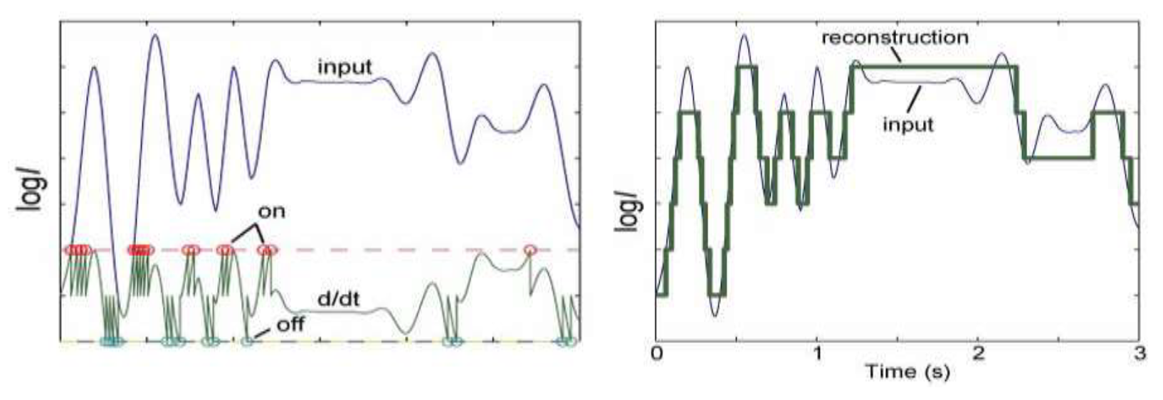
Figure 5.
EEG signals from EEG electrodes spatially distributed on the scalp are spatio-temporal signals (left figure). Each time series signal from an electrode is measured every 1 millisecond. The figure on the right shows the measurements of 14 EEG electrodes over 124 milliseconds. Each signal can be encoded into a 124-element vector according to Figure 4, making altogether 14 such vectors to be processed in the SAIN framework (reproduced from [11])
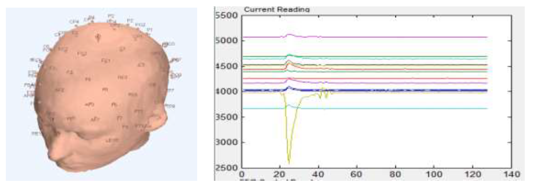
Figure 6.
ECG (Electro cardiogram) signals (a- nosy and b-filtered) can be encoded into binary vectors according to the spike encoding methods from Figure 4. Spike encoding is robust to noise, as any noise below a threshold would not cause the generation of a spike (either positive or negative), and the encoder will act as a filter. This vector’s length will equal the number of measurement time points. The vector data can be further processed in the SAIN framework
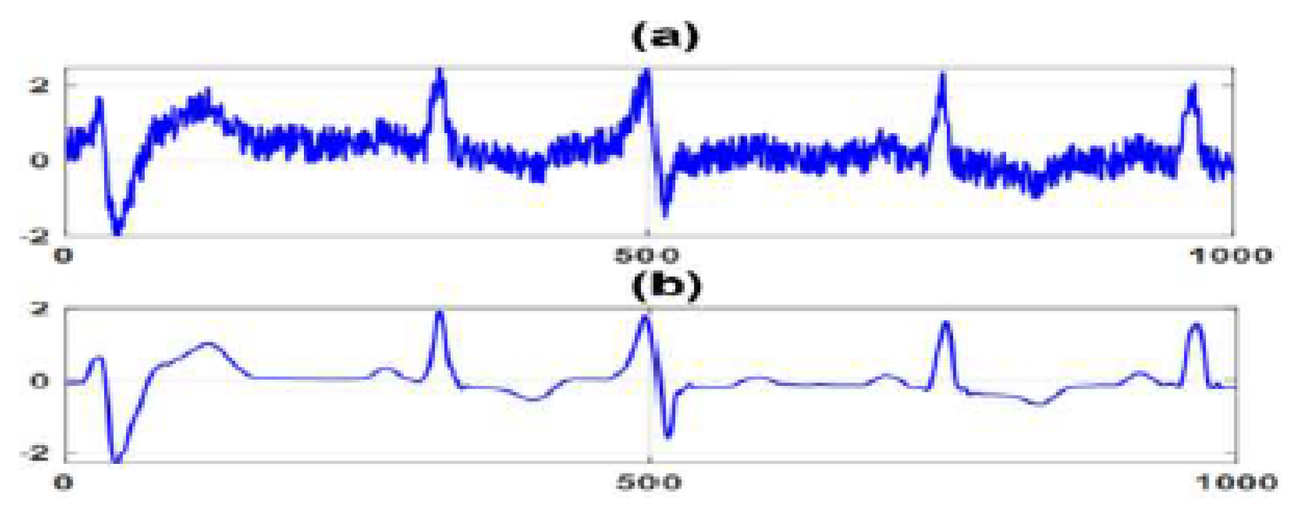
Figure 7.
Sample of the classification breakdown and the confusion matrix.
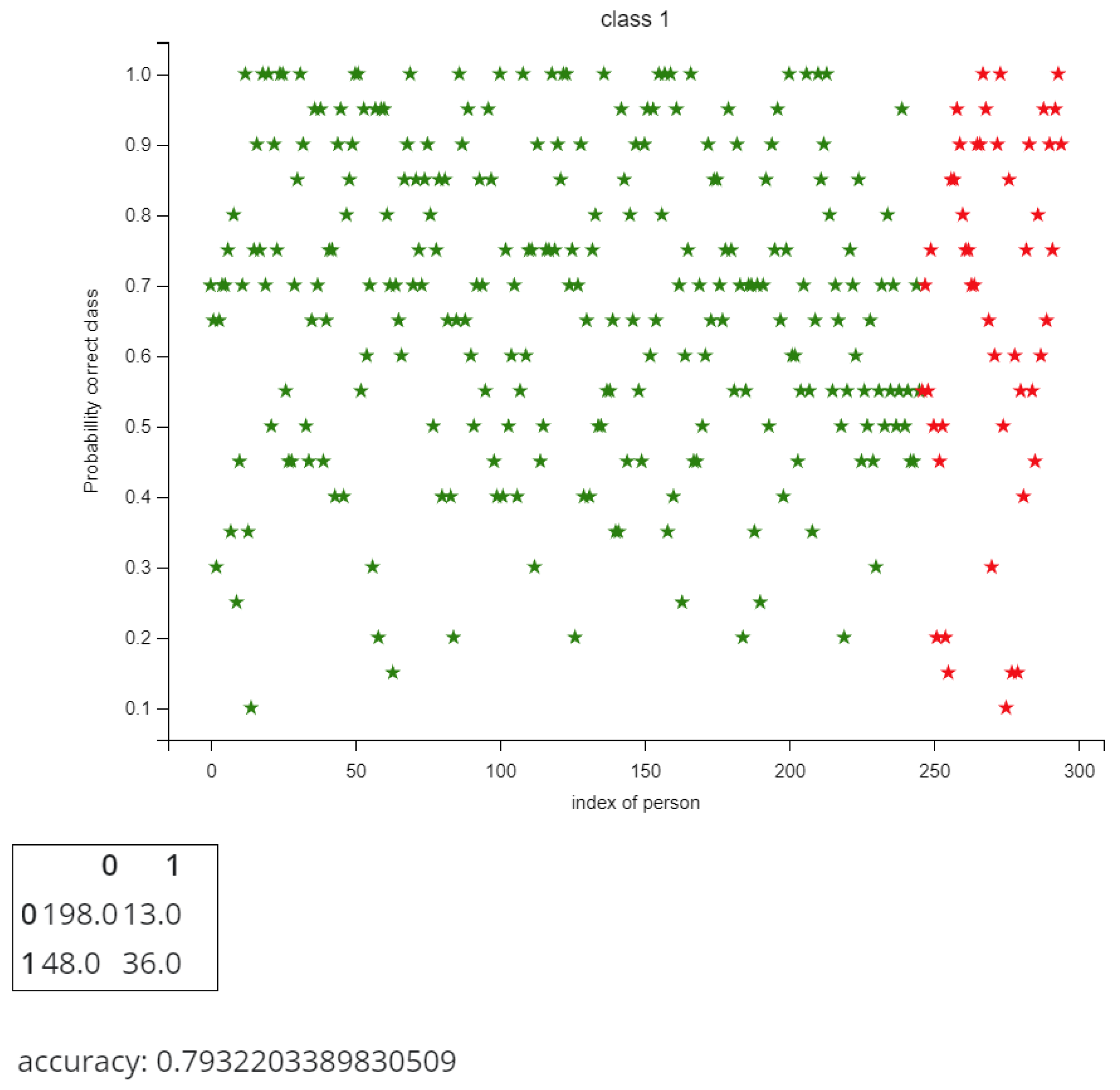

Table 1.
Unlabelled database
| Objects/Criteria | ... | ... | ||||
| ... | ... | |||||
| ⋮ | ⋮ | ⋮ | ... | ⋮ | ... | ⋮ |
| ... | ... | |||||
| ⋮ | ⋮ | ⋮ | ... | ⋮ | ... | ⋮ |
| ... | ... | |||||
| w | ... | ... |
Table 2.
Labelled database
| Objects/Criteria | ... | ... | Class label | ||||
| ... | ... | ||||||
| ⋮ | ⋮ | ⋮ | ... | ⋮ | ... | ⋮ | ⋮ |
| ... | ... | ||||||
| ⋮ | ⋮ | ⋮ | ... | ⋮ | ... | ⋮ | ⋮ |
| ... | ... |
Table 3.
Weights
| Criteria weights | ... | ... | ||||
| w | ... | ... |
Table 4.
New unlabelled object
| Object/Criteria | ... | ... | ||||
| x | ... | ... |
Table 5.
The hypothetical object
| Object/Criteria | ... | ... | Class label | ||||
| ... | ... |
Table 6.
Example of labelled data
| 68.2 | 0 | 6789 | small | red | 0,1,-1,-1,1,1,0,0, 1,-1 | 1,1,0 | 1 |
| 0,0,1 | |||||||
| 0,0,1 | |||||||
| 93 | 1 | 98000 | medium | yellow | 0,-1,-1,-1,-1,0,0, 1,-1,1 | 1,0,0 | 1 |
| 0,0,1 | |||||||
| 0,0,1 | |||||||
| 44.5 | 1 | 5600 | large | red | 0,1,-1,1,-1,1,0,0, 1,-1 | 1,1,0 | 1 |
| 1,0,1 | |||||||
| 1,1,1 | |||||||
| 56.8 | 0 | 89 | small | white | 1,-1,-1,-1,-1,1,0,0, 1,-1 | 1,1,0 | 1 |
| 0,1,1 | |||||||
| 1,0,1 | |||||||
| 26.3 | 0 | 9456 | large | black | 1,-1,-1,-1,0,1,0,0, 1,-1 | 1,1,0 | 2 |
| 1,1,1 | |||||||
| 1,0,1 | |||||||
| 81.5 | 1 | 78955 | medium | red | 0, 1,-1,1,-1,-1,0,0, 1,-1 | 1,1,0 | 2 |
| 0,0,1 | |||||||
| 1,1,1 | |||||||
| 56.7 | 1 | 68900 | small | black | 1,- 1,-1,1,-1,1,0,0, 1,1 | 1,1,1 | 2 |
| 0,0,1 | |||||||
| 1,1,1 | |||||||
| 20 | 0 | 7833 | large | yellow | 1,1,-1,-1,1,1,0,-1, -1,1 | 1,0,0 | 2 |
| 0,0,1 | |||||||
| 1,1,1 | |||||||
| 20 | 0 | 7833 | ∞ | yellow | 1,1,-1,-1,1,1,0,-1, -1,1 | 1,0,0 | 2 |
| 0,0,1 | |||||||
| 1,1,1 |
Table 7.
Example of new unlabelled object
| 48.5 | 1 | 45679 | large | red | 1, 0, 0, -1, 1, -1, 1, 0, 0, 1 | 1,1,0 |
| 0,0,1 | ||||||
| 1,0,1 |
Table 8.
Coded labelled data
| 68.2 | 0 | 6789 | 0 | FF0000 | 0122110012 | 110001001 | 1 | |
| 111111110000000000000000 | ||||||||
| 93 | 0 | 98000 | 1 | FFFF00 | 0222200121 | 110001001 | 1 | |
| 111111111111111100000000 | ||||||||
| 44.5 | 1 | 5600 | 2 | FF0000 | 0121210012 | 110101111 | 1 | |
| 111111110000000000000000 | ||||||||
| 56.8 | 0 | 89 | 0 | FFFFFF | 1222210012 | 110011101 | 1 | |
| 111111111111111111111111 | ||||||||
| 26.3 | 0 | 9456 | 2 | 000000 | 1222010012 | 110111101 | 2 | |
| 000000000000000000000000 | ||||||||
| 81.5 | 1 | 78955 | 1 | FF0000 | 0121220012 | 110001111 | 2 | |
| 111111110000000000000000 | ||||||||
| 56.7 | 1 | 68900 | 0 | 000000 | 1221210011 | 111001111 | 2 | |
| 000000000000000000000000 | ||||||||
| 20 | 0 | 7833 | 2 | FFFF00 | 1122110221 | 100001111 | 2 | |
| 111111111111111100000000 | ||||||||
| 20 | 0 | 7833 | ∞ | FFFF00 | 1122110221 | 100001111 | 2 | |
| 111111111111111100000000 |
Table 9.
New unlabelled object coded
| x | 48.5 | 1 | 45679 | 2 | FF0000 | 1002121001 | 110001101 |
| 111111110000000000000000 |
Table 10.
Coded labelled normalised data
| 0.682 | 0 | 0.06789 | 0 | 0.2 | 0.0122110012 | 0.110001001 | |
| 0.93 | 1 | 0.98 | 0.5 | 0.6 | 0.0222200121 | 0.100001001 | |
| 0.445 | 1 | 0.056 | 1 | 0.2 | 0.0121210012 | 0.110101111 | |
| 0.568 | 0 | 0.00089 | 0 | 1 | 0.1222210012 | 0.110011101 | |
| 0.263 | 0 | 0.09456 | 1 | 0 | 0.1222010012 | 0.110111101 | |
| 0.815 | 1 | 0.78955 | 0.5 | 0.2 | 0.0121220012 | 0.110001111 | |
| 0.567 | 1 | 0.689 | 0 | 0 | 0.1221210011 | 0.111001111 | |
| 0.2 | 0 | 0.07833 | 1 | 0.6 | 0.1122110221 | 0.100001111 | |
| 0.2 | 0 | 0.07833 | ∞ | 0.6 | 0.1122110221 | 0.100001111 |
Table 11.
New unlabelled object coded normalised
| x | 0.485 | 1 | 0.45679 | 1 | 0.2 | 0.1002121001 | 0.110001101 |
Table 12.
Normalised distances from the new object to all objects
| 0.197 | 1 | 0.3889 | 1 | 0 | 0.4 | 0.11111111 | 3.09701111 | |
| 0.445 | 0 | 0.52321 | 0.5 | 0.33333333 | 0.6 | 0.22222222 | 2.62376556 | |
| 0.04 | 0 | 0.40079 | 0 | 0 | 0.5 | 0.22222222 | 1.16301222 | |
| 0.083 | 1 | 0.4559 | 1 | 0.66666667 | 0.45 | 0.11111111 | 3.76667778 | |
| 0.222 | 1 | 0.36223 | 0 | 0.33333333 | 0.45 | 0.22222222 | 2.58978556 | |
| 0.33 | 0 | 0.33276 | 0.5 | 0 | 0.45 | 0.11111111 | 1.72387111 | |
| 0.082 | 0 | 0.23221 | 1 | 0.33333333 | 0.45 | 0.22222222 | 2.31976556 | |
| 0.285 | 1 | 0.37846 | 0 | 0.33333333 | 0.45 | 0.22222222 | 2.66901556 | |
| 0.285 | 1 | 0.37846 | 1 | 0.33333333 | 0.45 | 0.22222222 | 3.66901556 |
Table 13.
Ranking of distances in increasing order in Table 12
Table 13.
Ranking of distances in increasing order in Table 12
| 0.04 | 0 | 0.40079 | 0 | 0 | 0.5 | 0.22222222 | 1.16301222 | |
| 0.33 | 0 | 0.33276 | 0.5 | 0 | 0.45 | 0.11111111 | 1.72387111 | |
| 0.082 | 0 | 0.23221 | 1 | 0.33333333 | 0.45 | 0.22222222 | 2.31976556 | |
| 0.222 | 1 | 0.36223 | 0 | 0.33333333 | 0.45 | 0.22222222 | 2.58978556 | |
| 0.445 | 0 | 0.52321 | 0.5 | 0.33333333 | 0.6 | 0.22222222 | 2.62376556 | |
| 0.285 | 1 | 0.37846 | 0 | 0.33333333 | 0.45 | 0.22222222 | 2.66901556 | |
| 0.197 | 1 | 0.3889 | 1 | 0 | 0.4 | 0.11111111 | 3.09701111 | |
| 0.285 | 1 | 0.37846 | 1 | 0.33333333 | 0.45 | 0.22222222 | 3.66901556 | |
| 0.083 | 1 | 0.4559 | 1 | 0.66666667 | 0.45 | 0.11111111 | 3.76667778 |
Table 14.
An exemplar object
| 0.2 | 0 | 0.00089 | 0 | 1 | 0.1222210012 | 0.100001001 |
Table 15.
Vectors , rounded to two decimals
| 1.469 | 0.987 | 1.469 | 1.402 | 1.469 | 0.669 | 1.359 | 1.459 |
| 3.709 | 2.979 | 2.709 | 2.730 | 3.209 | 3.309 | 3.609 | 3.709 |
| 3.220 | 2.975 | 2.220 | 3.165 | 2.220 | 2.420 | 3.110 | 3.210 |
| 0.378 | 0.010 | 0.378 | 0.378 | 0.378 | 0.378 | 0.378 | 0.368 |
| 2.167 | 2.104 | 2.167 | 2.073 | 1.167 | 1.167 | 2.167 | 2.157 |
| 3.824 | 3.209 | 2.824 | 3.035 | 3.324 | 3.024 | 3.714 | 3.814 |
| 3.066 | 2.699 | 2.066 | 2.378 | 3.066 | 2.066 | 3.066 | 3.055 |
| 1.487 | 1.487 | 1.487 | 1.410 | 0.487 | 1.087 | 1.477 | 1.487 |
| 1.487 | 1.487 | 1.487 | 1.410 | 0.487 | 1.087 | 1.477 | 1.487 |
Table 16.
Distances and (normalised) weights
| Distances | 2.870 | 4.00 | 2.826 | 5.00 | 5.60 | 0.450 | 0.061 |
| Weights | 0.137 | 0.192 | 0.135 | 0.240 | 0.269 | 0.021 | 0.002 |
Table 17.
Survival database
| Patients/Criteria | ... | ... | Units of time | ||||
| ... | ... | ||||||
| ⋮ | ⋮ | ⋮ | ... | ⋮ | ... | ⋮ | ⋮ |
| ... | ... | ||||||
| ⋮ | ⋮ | ⋮ | ... | ⋮ | ... | ⋮ | ⋮ |
| ... | ... |
Table 18.
The new patient record
| Patient/Criteria | ... | ... | ||||
| p | ... | ... |
Table 19.
Patient records
| patients | units of time | |||||||
| 0.682 | 0 | 0.06789 | 0 | 0.2 | 0.012211001 | 0.110001001 | 12.3 | |
| 0.93 | 1 | 0.98 | 0.5 | 0.6 | 0.022220012 | 0.100001001 | 15 | |
| 0.445 | 1 | 0.056 | 1 | 0.2 | 0.012121001 | 0.110101111 | 68 | |
| 0.568 | 0 | 0.00089 | 0 | 1 | 0.122221001 | 0.110011101 | 1.4 | |
| 0.263 | 0 | 0.09456 | 1 | 0 | 0.122201001 | 0.110111101 | 40.5 | |
| 0.815 | 1 | 0.78955 | 0.5 | 0.2 | 0.012122001 | 0.110001111 | 97.2 | |
| 0.567 | 1 | 0.689 | 0 | 0 | 0.122121001 | 0.111001111 | 97.2 | |
| 0.2 | 0 | 0.07833 | 1 | 0.6 | 0.112211022 | 0.100001111 | 55.7 | |
| 0.2 | 0 | 0.07833 | ∞ | 0.6 | 0.112211022 | 0.100001111 | 63.7 |
Table 20.
New patient records
| 0.485 | 1 | 0.45679 | 1 | 0.2 | 0.1002121001 | 0.110001101 |
Table 21.
Distances between all patients and the new patient
| Distance d | ||||||||
| 0.1970 | 1 | 0.388900 | 1.0 | 0.0 | 0.08800109890 | 0.000000100 | 2.67390119890 | |
| 0.4450 | 0 | 0.523210 | 0.5 | 0.4 | 0.07799208800 | 0.010000100 | 1.95620218800 | |
| 0.0400 | 0 | 0.400790 | 0.0 | 0.0 | 0.08809109890 | 0.000100010 | 0.52898110890 | |
| 0.0830 | 1 | 0.455900 | 1.0 | 0.8 | 0.02200890110 | 0.000010000 | 3.36091890110 | |
| 0.2220 | 1 | 0.362230 | 0.0 | 0.2 | 0.02198890110 | 0.000110000 | 1.80632890110 | |
| 0.3300 | 0 | 0.332760 | 0.5 | 0.0 | 0.08809009890 | 0.000000010 | 1.25085010890 | |
| 0.0820 | 0 | 0.232210 | 1.0 | 0.2 | 0.02190890100 | 0.001000010 | 1.53711891100 | |
| 0.2850 | 1 | 0.378460 | 0.0 | 0.4 | 0.01199892200 | 0.009999990 | 2.08545891200 | |
| 0.2850 | 1 | 0.378460 | 1.0 | 0.4 | 0.01199892200 | 0.009999990 | 3.08545891200 |
Table 22.
The 14 variables used in the heart disease diagnosis case
| Name | Data type | Definition |
| age | integer | age in years |
| sex | binary | sex |
| cp | {1,2,3,4} | chest pain type |
| trestbps | integer | resting blood pressure |
| chol | integer | serum cholesterol in mg/dl |
| fbs | binary | fasting blood sugar > 120 mg/d |
| restecg | {0,1,2} | resting electrocardiographic results |
| thalach | I integer | maximum heart rate achieved |
| exang | binary | exercise-induced angina |
| oldpeak | float | ST depression induced by exercise relative to rest |
| slope | {1,2,3} | the slope of the peak exercise ST segment |
| ca | {0,1,2,3,} | number of major vessels colored by flourosopy |
| thal | {3,6,7} | heart status |
| num | {0,1,2,3,4} | diagnosis of heart disease |
Table 23.
Database of EEG records
| Record | Channel 1 | Channel 2 | Channel 3 | Label |
| R1 | (1, 1, -1, 0, 1) | (0, 1, 1, 1, -1) | (1, 1, -1, -1, 0) | 1 |
| R2 | (1, 0, -1, 0, 1) | ( 0, 1, 1, 1, -1) | (1, 0, -1, -1, 1 ) | 1 |
| R3 | (1, 1, -1, 0, 1) | (0, -1, 1, 1, -1) | (1, 1, -1, 0, 1) | 2 |
| R4 | (1, 1, -1, 0, 1) | (0, -1, 1, 0, -1) | (1, 1, -1, 0, 1) | 2 |
| R5 | (1, 1, -1, 0, 0) | (0, -1, 0, 1, -1) | (1, 1, -1, 1, 1) | 3 |
| R6 | (1, -1, -1, 0, 1) | (0, -1, 1, 0, -1) | (1, 1, -1, 0, 1) | 3 |
Disclaimer/Publisher’s Note: The statements, opinions and data contained in all publications are solely those of the individual author(s) and contributor(s) and not of MDPI and/or the editor(s). MDPI and/or the editor(s) disclaim responsibility for any injury to people or property resulting from any ideas, methods, instructions or products referred to in the content. |
© 2025 by the authors. Licensee MDPI, Basel, Switzerland. This article is an open access article distributed under the terms and conditions of the Creative Commons Attribution (CC BY) license (http://creativecommons.org/licenses/by/4.0/).
Copyright: This open access article is published under a Creative Commons CC BY 4.0 license, which permit the free download, distribution, and reuse, provided that the author and preprint are cited in any reuse.


