

Submitted:
27 June 2025
Posted:
01 July 2025
You are already at the latest version
Abstract
Addressing the imperative for energy transition amid depleting fossil fuels, distributed generation (DG) is increasingly integrated into distribution networks (DN). This integration necessitates low-carbon dispatching solutions that reconcile economic and environmental objectives. To bridge the gap between conventional “electricity perspective” optimization and emerging “carbon perspective” requirements, this research integrated Carbon Emission Flow (CEF) theory to analyze spatiotemporal carbon flow characteristics within DN. Recognizing the limitations of single-objective approached in balancing multifaceted demands, a multi-objective optimization model was formulated. This model could capture the spatiotemporal dynamics of nodal carbon intensity for low-carbon dispatching while comprehensively incorporating diverse operational economic costs to achieve collaborative low-carbon and economic dispatch in DG-embedded DN. To efficiently solve this complex constrained model, a novel Q-learning enhanced Moth Flame Optimization (QMFO) algorithm was proposed. QMFO synergized the global search capability of the Moth Flame Optimization (MFO) algorithm with the adaptive decision-making of Q-learning, embedding an adaptive exploration strategy to significantly enhance solution efficiency and accuracy for multi-objective problems. Validated on a 16-node three-feeder system, the method co-optimizes switch configurations and DG outputs, achieving dual objectives of loss reduction and carbon emission mitigation while preserving radial topology feasibility.
Keywords:
distribution networks
; carbon emission flow
; topology reconfiguration
; distributed generation
; forward/backward sweep
; Q-learning enhanced moth-flame optimization
1. Introduction
Achieving the “Dual Carbon” goals necessitates deep decarbonization in the energy sector. High-penetration distributed generation (DG) integration into distribution networks (DN) is pivotal for boosting renewable consumption, improving efficiency, reducing carbon costs, and increasing system flexibility. However, DG introduces significant challenges: its power uncertainty and potential backflow transform power flow from unidirectional to bidirectional, causing voltage fluctuations, increased losses, and protection coordination issues. The dynamic topology changes induced by increasing DG penetration render traditional static reconfiguration methods inadequate for real-time optimization. Furthermore, DG integration often creates conflicts between loss minimization and operational cost reduction objectives, highlighting the essential role of multi-objective optimization.
Research on DG and system reconfiguration has alleviated power supply pressure, enhanced DN stability, and reduced carbon costs. Yet, DG integration demands continuous grid optimization for flexibility, reliability, and DG management. Methods like the improved plant growth simulation algorithm for reconfiguration effectively reduce losses and support real-time DN control [1], emphasizing the need for integrated economic and technical feasibility to ensure stability. Equivalent modeling approaches, such as clustering DGs based on control parameters and grid strength [2], and measurement-based methods (e.g., generalized load, ADN, or MG models [3]) leveraging system identification or Monte Carlo sampling [4], address the challenges of simulating DG in large grids.
However, existing stability and reconfiguration optimizations often adopt a purely “power system perspective”, minimizing losses and costs while overlooking carbon emission costs. This separation between “power system” and “carbon” perspectives compromises overall system economy and low-carbon performance. Integrating these perspectives is crucial, as carbon emission measurement and allocation underpin low-carbon power system technologies [5]. The interaction between electricity and carbon markets enables multi-area systems to participate in centralized or decentralized trading. While decentralized peer-to-peer (P2P) electricity-carbon trading offers flexibility and privacy, research focuses on secure algorithms and risk assessment, with approaches like consensus-based adaptive ADMM needing further refinement to include grid constraints and purchased electricity emissions [6].
Carbon Emission Flow (CEF) theory provides a vital analytical tool for low-carbon DN dispatch, quantifying emissions across nodes and branches by tracking power flow paths and intensity [7]. Unlike carbon emission trading (CET) mechanisms suited for IES or MGs, CEF is essential for DNs due to their complex structure, multi-source/multi-load nature, bidirectional flow, and uncertainty. CEF modeling, including considerations for power quality [8], guides clean energy configuration and prioritization, improving system efficiency and cleanliness by reducing high-carbon energy transmission paths.
DN reconfiguration—optimizing topology via switch adjustments—improves economy, reliability, cost, power flow, and reduces losses. It can be static (single time-section) or dynamic (multiple periods for global optimization) [9], with heuristic algorithms proposed for both [10,11]. Increasing DG penetration has shifted reconfiguration research from single-objective to multi-objective optimization, balancing losses, DG connection/operation, and maintenance topology changes. Addressing DG’s negative impacts (e.g., voltage fluctuations via reactive power control [12]) and leveraging reconfiguration for load/flow management are critical. Crucially, network reconfiguration underpins CEF analysis and optimization [13].
Under the “Dual Carbon” imperative, CEF and economic flow are key reconfiguration objectives. Many studies incorporate carbon reduction into multi-objective optimization, such as low-carbon economic dispatch models using CEF theory and Demand Response (DR) to reduce peak-valley differences and enhance wind consumption, optimizing both supply and carbon trading costs [14]. Research also examines DG’s impact on CEF [15]. Consequently, optimal power flow studies now encompass economic cost, system loss minimization, and carbon reduction [16].
Evolving optimization objectives and power flow dynamics drive exploration of new frameworks like deep learning and machine learning for complex DN stability and uncertainty. Algorithmic advances include Binary PSO for loss reduction and combined DG-ES reconfiguration [17], MIQP for improved convergence and accuracy in reconfiguration and reactive power optimization [18], and optimal power flow-based controls mitigating voltage violations from high DG penetration [19]. Distributed power flow methods break distance limitations for global planning and stability assessment [20], while two-layer structures optimize DG/ES via DR, considering power market-thermal system interactions [21], and schemes optimally adjust ES/DG flow to reduce costs and enhance reliability/safety [22].
In summary, as DG’s role in DNs expands, topological reconfiguration optimization research is vital for enhancing DN economy and stability, and critical for achieving low-carbon goals. Multi-objective optimization, driven by the “Dual Carbon” target, is essential for sustainable DN development. To address the above challenges, realize low-carbon economic DN dispatch, promote renewable energy consumption, and coordinate complex interactions between DNs and users, this research contributes as follows:
- Integrated Carbon-Electricity Framework in DN: Bridges the “electricity” and “carbon” perspectives via CEF theory for low-carbon economic DG-integrated DN reconfiguration;
- Spatiotemporal Multi-Objective Optimization Model: Addressing the limitation of single-objective optimization in balancing competing requirements, a multi-objective model for DN topology reconfiguration was constructed which could enable collaborative low-carbon and economic dispatch for DG-integrated DN systems;
- Novel Q-Learning Enhanced MFO Algorithm (QMFO): Proposed Q-learning enhanced Moth Flame Optimization with adaptive exploration for efficient, accurate solution of the complex scheduling model.
2. Energy Flow in Distribution Network
2.1. Power Flow Calculation
Although this research has taken carbon flow as the main research objective for analysis and optimization, power flow in the distribution network remains a necessary and fundamental existence.
Given the radial topology of typical distribution networks and limited node counts per feeder, Forward/Backward Sweep (FBS) method was adopted with integrated DG modeling. Specifically designed for radial systems, FBS leverages structural simplicity by eliminating Jacobian matrix construction and inversion requirements of transmission-oriented methods like Newton-Raphson. The algorithm iterates through: (1) Backward Sweep: Computes branch power flows and losses from leaf nodes toward the substation; (2) Forward Sweep: Updates node voltages from the substation toward leaf nodes [23].
2.1.1. General Forward/Backward Sweep Method
The FBS algorithm proceeds iteratively until convergence is achieved:
- Backward Sweep (Power Summation): Starting from the leaf nodes (end nodes) and moving backwards towards the root node, calculate the power flow in each branch. For each node j (starting from end nodes):where is the total complex power flow through node i; is the load power at node i; is the set of child nodes connected to i; is the current in branch ; is the voltage at child node j; is the branch impedance and its complex form.
- Forward Sweep (Voltage Update): Starting from the root node and moving forward towards the leaf nodes, update the voltage at each node using the branch currents/powers calculated in the backward sweep. For each node j (starting from root):where ; is the updated voltage at the child node j; is the voltage at the parent node i.
- Convergence Check: Check if the change in node voltages between consecutive iterations is below a specified tolerance:where is the voltage magnitude at node i, iteration m; is the convergence tolerance.
- Loss Calculation (Post-Processing): For each branch :where is the active power loss in branch ; is the reactive power loss in branch .
2.1.2. Processing Method for Nodes with DGs
The access of DGs changes the power flow distribution in the system, which can reduce the current of each branch in the distribution network and thereby decrease the power loss of the overall system. Meanwhile, with DGs integrated, the risk-resistance capacity of the system can be significantly improved.
The combined deployment of gas turbine (GT) and distributed PV systems constitutes a frequently implemented solution in contemporary distribution networks, especially among energy-intensive consumers such as medium-sized industrial parks. This research therefore prioritizes modeling these two key DG technologies.
For GTs, the excitation regulation capability of synchronous motors can ensure stable P and V, so it can be regarded as a power supply model with constant P and V. At the beginning of the iteration, the reactive power of this node can be set according to Equation 5, so that the active power output remains unchanged and the port voltage remains constant:
where represents the initial iteration of ; and represent the upper and lower boundary of the reactive power at node i.
When calculating at the mth iteration, the initialized current injected into this node is:
Grid-connected distributed photovoltaic systems typically adopt either voltage-mode or current-mode control. Compared to voltage-mode control, which is susceptible to grid voltage fluctuations, current-mode control regulates the output current with minimal interference from grid voltage variations, thereby mitigating the impact of voltage disturbances on current output and improving power quality. Additionally, current-mode control offers advantages such as simple structure, fast response, and high sinusoidal waveform fidelity, making it widely used in practical applications [24]. Therefore, this research employs a current-controlled inverter for grid integration, which can be regarded as a power supply model with constant P and I, with the calculation method below:
where and are the active power and output current provided by the distributed PV respectively, and the output reactive power of the PV can be calculated as:
2.2. Carbon Emission Flow Theory
Carbon emission flow theory fundamentally extends power flow theory. As established in power flow analysis, determining a system’s operational state relies on predefined operating conditions and network topology. Similarly, CEF quantification operates analogously: it dynamically traces carbon emission flows within a power system based on the underlying power flow distribution [25]. Carbon emissions are intrinsically coupled with power flows—any factor altering power flow inevitably impacts carbon flow. However, CEF also exhibits unique properties influenced by non-power-flow factors beyond conventional system boundaries.
In the theory of CEF, nodal carbon intensity and branch carbon flow density are two key fundamental factors that constitute the theory of carbon emission flow. The nodal carbon intensity is defined as:
where is the nodal carbon intensity at node i; is the carbon flow injected to node i; is the active power injected to node i; is the generator power output at node i.
Nodal carbon intensity describes the carbon emission intensity per unit of electrical energy at a node, similar to the concept of voltage in a circuit. Voltage is the potential difference that drives the flow of charges, while carbon intensity is the “carbon pressure difference” that drives the transfer of carbon emission responsibility.
The branch carbon flow density is defined as:
where is the branch carbon flow density in branch ; is the power flow in branch .
Carbon flow density describes the absolute carbon emissions of electrical energy transmitted by a branch, similar to the concept of current in a circuit. Current represents the amount of charges passing through a conductor per unit time, while carbon flow density represents the carbon emissions passing through a branch per unit time.
The carbon emission flow in the power system depends on the injection power to the node and is independent of the outflow power from the node [7]. denotes the active power flux of the node. Define the set of upstream branches of node i as B, then
where s represents the sth upstream branch of node i, and the end node of this branch is node i.
If the carbon emission intensity of DGs is defined as the vector and the nodal carbon intensity vector of all nodes is defined as , then the formula of node nodal carbon intensity can be rewritten in matrix form:
3. Topology Reconfiguration via Power Loss Minimization
The reduction of active power losses constitutes a primary objective in distribution network topology reconfiguration. The optimization target for power loss reduction is formulated as:
where D denotes the set of nodes transferred from the original feeder, M and N represent the start and end bus nodes of the tie switch along the radial power flow direction, signifies the current at bus i, is the loop resistance between reconfigured feeders, while and indicate voltages at the respective start and end nodes [26].
Under full reactive power compensation conditions, the power loss function exhibits distinct mathematical properties enabling computational optimization. Analysis reveals that possesses both unimodal and quadratic characteristics:
These properties permit closed-form identification of the optimal sectionalizing switch for loss minimization. The minimal active power loss is derived as:
This fundamental relationship enables deterministic selection of sectionalizing switches to open and tie switches to close, achieving preliminary topology optimization through targeted loss reduction.
The formulation provides theoretical guarantees for radial topology feasibility while offering computational efficiency advantages over heuristic search methods. The quadratic structure ensures convergence to global minima within the solution space, making it particularly suitable for real-time reconfiguration applications in active distribution networks.
4. Low-Carbon Optimal Dispatch Model
4.1. Objective Function
The low-carbon optimal dispatch model integrates multiple cost components to achieve economic and environmental optimization. Carbon emission costs form a critical component of this optimization framework, calculated based on node-specific carbon potential and load consumption patterns. The carbon emission cost is determined as follows:
where represents the branch power flow distribution matrix; denotes the branch carbon flow rate distribution matrix; is the active load at node i during time t; signifies the carbon potential at node i and time t. This formulation captures the spatial and temporal variations in carbon intensity throughout the distribution network.
Economic grid costs incorporate several operational factors, including electricity procurement, line losses, and DG contributions. The comprehensive economic cost formulation accounts for these elements:
Here, indicates the electricity purchase price, represents the total absorbed load power, quantifies active power losses in distribution lines, aggregates photovoltaic output, and measures GT output. This expression reflects the net economic impact of generation and consumption patterns.
Fuel consumption costs directly relate to GT operation, with efficiency considerations embedded in the formulation:
where denotes the electrical power generated per ton of fuel, T represents total fuel tonnage, and is the unit fuel cost. This cost component incentivizes efficient fuel utilization during GT dispatch.
The complete objective function combines these cost elements through weighted aggregation:
Weight coefficients , , and balance environmental, economic, and fuel efficiency objectives, satisfying to maintain proportionality in the multi-objective optimization. This integrated approach enables Pareto-optimal solutions that harmonize carbon reduction with operational economics.
4.2. Constraints
Power flow constraints ensure stable network operation within technical limits. Voltage magnitudes at PQ nodes must remain within specified boundaries:
where and define the lower and upper voltage limits respectively. This constraint preserves voltage quality and prevents equipment damage from overvoltage or undervoltage conditions.
Voltage phase angle differences between adjacent nodes are constrained to maintain stability:
where and represent voltage phase angles at nodes i and j, while denotes the maximum allowable phase difference. This limitation prevents excessive power angle disparities that could compromise system synchronization.
PV generation adheres to physical and operational limitations, with output constrained by both device capabilities and grid integration policies:
PV generation output is rigorously bounded with dual operational constraints: the system’s physical capacity and the policy-based grid integration ceiling , where represents the penetration factor of the PV output, ensuring compliance with both technical specifications and grid stability requirements.
GT operation respects load-following capabilities while preventing reverse power flow:
where represents the load at the generator’s connection node.
Carbon potential constraint drives the optimization toward environmentally favorable configurations:
By limiting node carbon intensity below threshold , this constraint actively promotes topology reconfigurations that reduce carbon footprints. The mechanism aligns technical loss reduction with climate policy objectives, creating synergistic benefits across operational domains.
5. Solution Method of Low-carbon Dispatch Model
5.1. Moth Flame Optimization Algorithm
The Moth Flame Optimization algorithm (MFO) demonstrates exceptional global optimization capability and high-precision convergence for constrained problems with unknown search spaces [27]. Inspired by moths’ celestial navigation mechanism, MFO mathematically models their lateral positioning behavior where flight paths are continuously adjusted based on relative light angles. When approaching artificial flames in the algorithm, moths maintain fixed angular trajectories that generate logarithmic spiral convergence patterns, as illustrated in Figure 1.
MFO represents candidate solutions as moths, where each moth’s position in the search space corresponds to a solution vector. The population of n moths in d-dimensional space is represented by the matrix:
where d denotes the number of control variables to be optimized.
Each moth updates its position relative to a corresponding flame, with flame positions represented by an analogous matrix:
The position update mechanism follows:
where is the position of the i-th moth; is the j-th flame (the best-known position); S is the spiral search function that guides solution exploration.
The logarithmic spiral function S satisfies three fundamental properties:
- Origin: Starts at the moth’s current position;
- Terminus: Converges at the flame position;
- Boundedness: Fluctuations constrained within the search space.
The spiral function is mathematically defined as:
where is the Euclidean distance between moth i and flame j; b is a constant defining the spiral’s shape (convergence rate); is a random parameter controlling proximity to the flame.
This spiral dynamics balances exploration and exploitation, enabling effective navigation through complex solution spaces.
5.2. Q-learning Algorithm for Power System Optimization
Q-learning is a model-free reinforcement learning algorithm that enables autonomous decision-making in complex environments like power systems. By iteratively updating a state-action value function (Q-function), it learns optimal policies for energy management and dispatch problems [28]. The algorithm operates within a Markov Decision Process (MDP) framework (shown in Figure 2), where agents interact with their environment, receive rewards, and adjust actions to maximize long-term cumulative returns. Our implementation enhances traditional Q-learning with double Q-table learning for stability and adaptive exploration for faster convergence.
5.2.1. Markov Decision Process Components
The optimization framework adopts a MDP formulation with five fundamental elements that collectively define the decision-making environment. The state space comprehensively describes the power system’s operational status through a state vector composed of voltage magnitudes (V), active and reactive load values ( and ), and binary switch status indicators () [29]. This state representation follows the mathematical formulation:
with dimensionality determined by system components
where , , and respectively denote node count, controllable switches, and DG units. The Markov property inherent in this formulation ensures system evolution depends solely on the current state.
Control actions available to the agent are defined within the action space , which encompasses both topology reconfiguration through switch operations and DG power output adjustments. When executed, these actions trigger state transitions governed by the transition function . The model in this research employs deterministic state transitions based on power flow physics:
where represents the power flow solution mapping that uniquely determines the subsequent state given current conditions and actions.
Immediate performance feedback is provided through a reward function designed to penalize undesirable operational outcomes. This function combines two critical operational metrics:
where quantifies power losses and measures voltage deviation severity. Weighting coefficients and balance these competing objectives according to operational priorities. The negative sign ensures appropriate penalties for suboptimal conditions, steering the agent toward solutions that simultaneously enhance efficiency and power quality.
The temporal aspect of decision-making is modulated by the discount factor , which balances immediate rewards against future consequences. Higher values emphasize long-term strategic outcomes, while lower values prioritize near-term optimization benefits, creating a flexible mechanism for aligning solution horizons with operational requirements.
5.2.2. Q-value Learning Mechanism
Q-learning discovers optimal actions through iterative updates of the action-value function. The core update rule combines immediate rewards with estimated future values:
The learning rate controls update magnitude, balancing new information against existing knowledge. Convergence to the optimal requires two conditions: exhaustive exploration of all state-action pairs, and learning rate decay satisfying the Robbins-Monro conditions:
To mitigate maximization bias, we implement double Q-learning. This approach uses dual estimators that alternate updates, improving stability and reducing value overestimation.
5.2.3. Adaptive Exploration Strategy
The -greedy strategy balances exploration of novel actions against exploitation of known rewards through probabilistic action selection:
An adaptive exploration mechanism dynamically modulates the exploration rate over time according to the exponential decay formula:
Here represents the initial exploration probability, denotes the minimum sustained exploration rate, and controls the decay speed [30,31]. This approach guarantees comprehensive exploration during early learning phases while systematically transitioning toward exploitation as policy knowledge matures. The decaying exploration schedule prevents premature convergence to suboptimal policies while maintaining ongoing discovery potential throughout the learning process.
5.3. Q-learning Enhanced Moth-Flame Optimization
The Q-learning enhanced MFO algorithm establishes a coevolutionary framework integrating MFO and Q-learning, specifically designed for carbon-minimizing topology reconfiguration in distribution networks. This architecture leverages MFO’s population-based exploration to generate diverse radial topologies while embedding carbon-aware reward shaping within Q-learning’s policy optimization—directly linking switching actions to emission reduction through carbon flow tracing. Key innovations include: 1) Flame-directed Q-table updates that bias exploration toward low-carbon configurations; 2) Constraint-preserving action space encoding ensuring radial topology feasibility; 3) Dual convergence criteria (population entropy stability and Bellman residual minimization) certifying solution robustness.
Theoretically, QMFO resolves the combinatorial-explosion challenge in switch optimization by decomposing high-dimensional search spaces into cooperative subpopulations, while its carbon-electricity coupling mechanism enables Pareto-optimal tradeoffs between emission reduction and operational costs. This biologically-inspired paradigm fundamentally advances distribution network optimization by simultaneously addressing topological, environmental, and physical constraints. Figure A1 is a detailed flowchart of the QMFO algorithm formed on the model constructed in this research.
6. Case Study
6.1. 16-node Three-feeder model
The method of topology reconstruction was explained by taking the three-feeder model as the main model, detailed parameters could be found in [32]. This model consisted of 16 nodes and 3 tie switches (15, 21, 26) and 14 sectionalizing switches (11, 12, 13, 14, 16, 17, 18, 19, 20, 22, 23, 24, 25), as shown in the Figure 3.
As a medium and small-sized distribution network system, the reference voltage of this distribution network model was 23 kV and the reference capacity was 100 MVA.
It could be known from previous description:
- The electromotive force at Node 11 is greater than that at Node.5. In this case, the connecting switch that needs to be closed is 15. At this time, the alternative options that can conform to the are: opening the segmented Switch 16, 18 or 19, totaling three options;
- The electromotive force at Node 10 is greater than that at Node.14. In this case, the connecting switch that needs to be closed is 21. At this time, the alternative options that can conform to the are: opening the segmented switch 16 or 17, totaling two options;
- The electromotive force at Node 7 is greater than that at Node.16. In this case, the connecting switch that needs to be closed is 26. At this time, the alternative options that can conform to the are: opening the segmented Switch 11, 13 or 14, totaling three options.
3 connection switches and 14 section switches, these 8 different combinations could form 47 reasonable topological structures. Assume all feeders could always work functionally. It was necessary to conduct a preliminary screening of all 47 topological structures. The screening principle was straightforward: no feeder could be unloaded.
The purpose of this principle was obvious. If not all the feeders are loaded, on the one hand, the feeders are not effectively utilized; on the other hand, the line loss will increase significantly, which does not conform to the topology optimization objective of this research. In that case, 17 topology structures out of 47 were selected, which could be seen in Figure A2. These topologies exhibited tree-structured configurations with balanced node distribution across feeders.
6.2. Cases and Results
Three Cases were designed for comparison in this study (Table 1).
PV units and GT are integrated as DGs within the model, strategically positioned based on nodal load analysis. High-capacity PV systems, 15 MW in total, were allocated to major load buses (Node 6, 9, and 12) with, while a 12 MW GT was deployed at Node 5. Climate data for Weifang, Shandong’s medium-high voltage industrial park was sourced from NASA, enabling hourly PV output calculations. Both Case 1 and Case 2 adopt the Topology 6 in Figure A2, as shown in Figure 4. This topology is the optimal one without DGs. Case 3, however, uses the reconstruction model proposed in this study for low-carbon dispatch optimization. The results of the three schemes are shown in Table 2.
Figure 5 is the energy injection comparison of three cases above.
6.3. Result Analysis
Comprehensive case analysis confirm that the Case 3 distribution network model achieves significant reductions in carbon emissions (9.9%), economic costs (9.8%), and power losses (48%) compared to Case 1. This corresponds to absolute reductions of 3.386 million kgCO2 and 4.775 million CNY respectively. Further improvements are observed relative to Case 2, with additional reductions of 887,000 kgCO2 (2.8%) in emissions and 886,000 CNY (1.98%) in costs, alongside 37.7% lower line losses. These enhancements demonstrate Case 3’s superior capability to minimize transmission losses while maintaining minimum topological entropy under identical photovoltaic conditions.
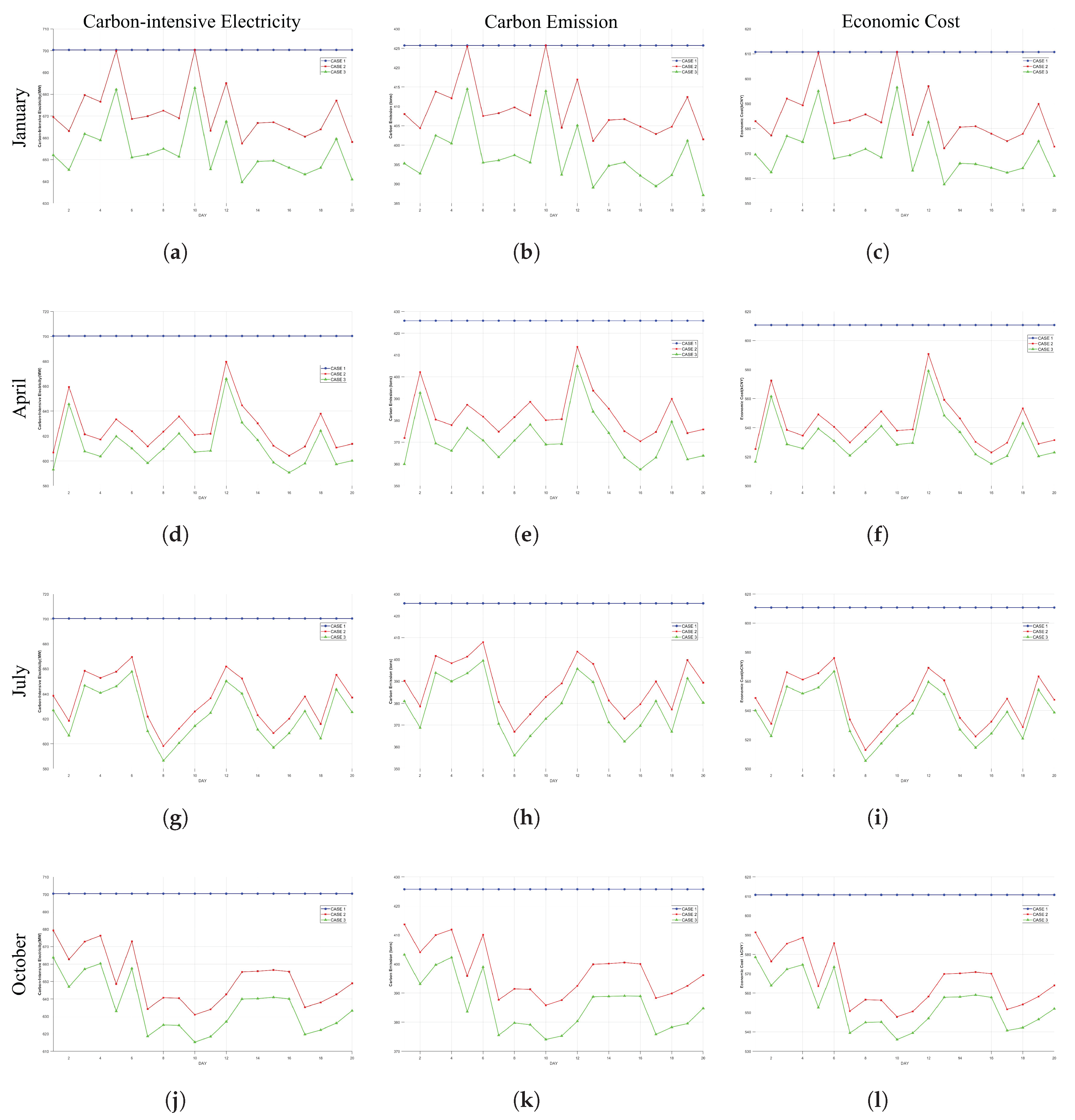
Seasonal performance analysis (Figure A3) reveals nuanced carbon reduction patterns: Winter operations show modest improvements due to reduced solar irradiance and increased gas turbine dependency, while spring achieves maximum emission reductions (2.218-2.422 million kgCO2 beyond Case 2) through optimal PV utilization and peak shaving. Summer maintains substantial gains despite slightly weaker irradiation, whereas autumn exhibits diminished margins due to increased turbine compensation. Economically, Case 3 delivers consistent cost advantages across seasons: 6.6% reduction in winter, 12.5% in spring, 11% in summer, and 9.2% in autumn relative to baseline, primarily through reduced grid procurement during high-PV periods.
The three-dimensional optimization framework simultaneously coordinates: 1) Topological reconfiguration for loss minimization; 2) Dynamic GT dispatch balancing PV fluctuations; 3) Strategic PV integration maximizing renewable utilization. This integrated approach establishes a global optimum with 48% power loss reduction, 9.9% emission decrease, and 9.8% cost savings, effectively addressing climate challenges through technical and operational synergies.
7. Conclusions
Against the backdrop of fossil fuel scarcity and energy transition, integrating DG into DN called for low-carbon dispatching. This study applied CEF theory to align traditional “electricity” and new “carbon” optimization approaches. A multi-objective model was created to track nodal carbon intensity and account for economic costs, achieving coordinated low-carbon and economic dispatch in DG-integrated DN. To solve the model, a QMFO algorithm was developed by merging MFO’s global search with Q-learning’s adaptability. Testing on a 16-node system confirmed that the approach optimized switch settings and DG outputs, reducing losses and emissions while keeping the radial network structure. The following conclusions could be drawn:
- By introducing the carbon flow theory and integrating the electricity-oriented and carbon-oriented perspectives, low carbon dispatching of the distribution network system was effectively achieved. Coupled with the distribution network reconfiguration method, low carbon operation of the distribution network was realized;
- A multi-objective DN topology reconfiguration model was constructed, which took into account both the economic efficiency and low carbon characteristics of distribution network dispatching;
- The QMFO algorithm was proposed, enabling effective solution of the proposed model.
Author Contributions
Conceptualization, R.F. and S.H.; methodology, R.F. and G.X.; software, G.X. and Y.Z.; validation, J.S. and R.F.; visualization, H.L. All authors have read and agreed to the published version of the manuscript.
Funding
This research was funded by Doctoral Fund Project of Shandong Jianzhu University, X21103Z.
Data Availability Statement
The original contributions presented in this study are included in the article. Further inquiries can be directed to the corresponding author.
Conflicts of Interest
The authors declare no conflicts of interest.
Appendix A
Figure A1.
QMFO flow chart.
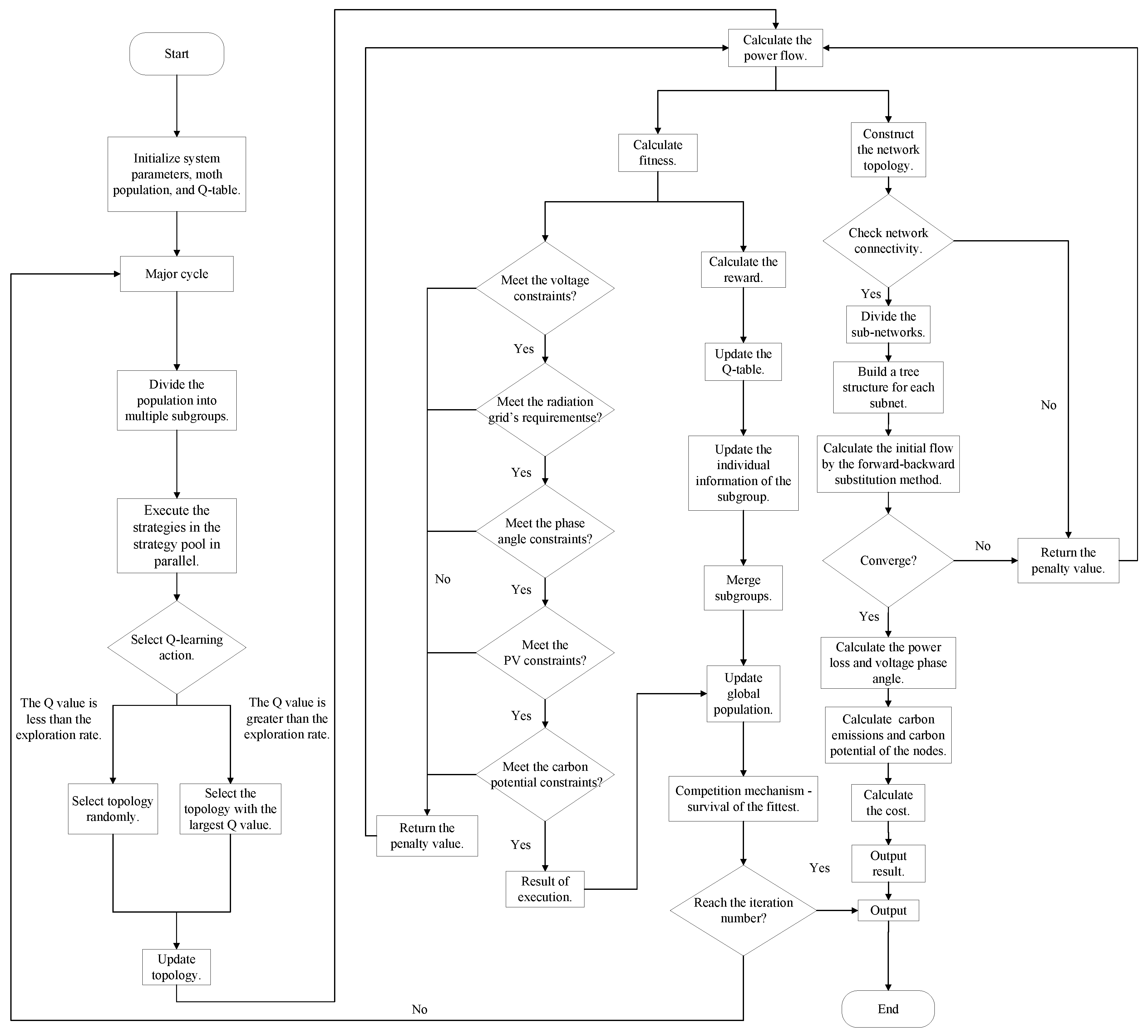
Figure A2.
17 reconfigured topology structures.
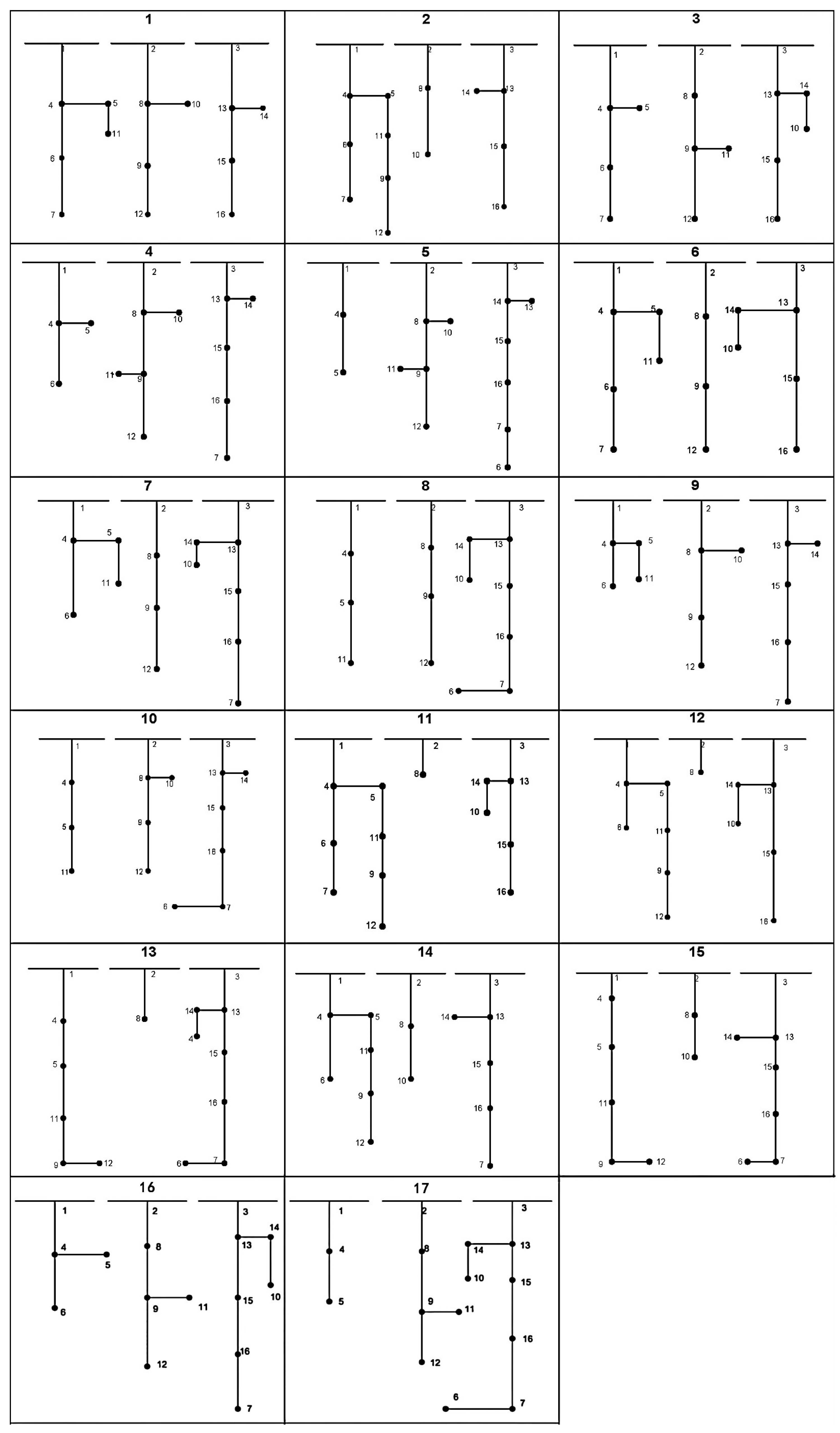
Figure A3.
Performance of three cases in different seasons.
References
- Rajaram, R.; Kumar, K.S.; Rajasekar, N. Power system reconfiguration in a radial distribution network for reducing losses and to improve voltage profile using modified plant growth simulation algorithm with Distributed Generation (DG). Energy Reports 2015, 1, 116–122. [Google Scholar] [CrossRef]
- Zhou, Y.; Zhao, L.; Lee, W.J. Robustness analysis of dynamic equivalent model of DFIG wind farm for stability study. IEEE Transactions on Industry Applications 2018, 54, 5682–5690. [Google Scholar] [CrossRef]
- Arif, A.; Wang, Z.; Wang, J.; Mather, B.; Bashualdo, H.; Zhao, D. Load modeling—A review. IEEE Transactions on Smart Grid 2017, 9, 5986–5999. [Google Scholar] [CrossRef]
- Chaspierre, G.; Denis, G.; Panciatici, P.; Van Cutsem, T. An active distribution network equivalent derived from large-disturbance simulations with uncertainty. IEEE Transactions on Smart Grid 2020, 11, 4749–4759. [Google Scholar] [CrossRef]
- Chen, S.; Sun, B.; He, Z.; Wu, Z. Calculation method of carbon emission flow in power system based on the theory of power flow calculation. In Proceedings of the 2015 6th international conference on manufacturing science and engineering. Atlantis Press, 2015, pp. 443–450.
- Wang, Y.; Hu, J. Peer-to-peer Energy-carbon Management Method of Multiple Integrated Energy Systems Considering Multi-agent Interaction Strategy. Journal of System Simulation 2024, 36, 2488–2502. [Google Scholar]
- Kang, C.; Zhou, T.; Chen, Q.; Wang, J.; Sun, Y.; Xia, Q.; Yan, H. Carbon emission flow from generation to demand: A network-based model. IEEE transactions on smart grid 2015, 6, 2386–2394. [Google Scholar] [CrossRef]
- Li, J.; Zhou, Z.; Wen, B.; Zhang, X.; Wen, M.; Huang, H.; Yu, Z.; Liu, Y. Modeling and analysis method for carbon emission flow in integrated energy systems considering energy quality. Energy Science & Engineering 2024, 12, 2405–2425. [Google Scholar]
- Peng, C.; Xu, L.; Gong, X.; Sun, H.; Pan, L. Molecular evolution based dynamic reconfiguration of distribution networks with DGs considering three-phase balance and switching times. IEEE Transactions on Industrial Informatics 2018, 15, 1866–1876. [Google Scholar] [CrossRef]
- Wang, H.J.; Pan, J.S.; Nguyen, T.T.; Weng, S. Distribution network reconfiguration with distributed generation based on parallel slime mould algorithm. Energy 2022, 244, 123011. [Google Scholar] [CrossRef]
- Li, Z.; Wang, S.; Zhou, Y.; Liu, W.; Zheng, X. Optimal distribution systems operation in the presence of wind power by coordinating network reconfiguration and demand response. International Journal of Electrical Power & Energy Systems 2020, 119, 105911. [Google Scholar]
- Wagle, R.; Sharma, P.; Sharma, C.; Amin, M.; Rueda, J.L.; Gonzalez-Longatt, F. Optimal power flow-based reactive power control in smart distribution network using real-time cyber-physical co-simulation framework. IET Generation, Transmission & Distribution 2023, 17, 4489–4502. [Google Scholar]
- Liu, Z.; Xing, H.; Luo, Y.; Ye, Y.; Shi, Y. Low-carbon economic dispatch of an integrated energy system based on carbon emission flow theory. Journal of Electrical Engineering & Technology 2023, 18, 1613–1624. [Google Scholar]
- Feng, J.; Nan, J.; Wang, C.; Sun, K.; Deng, X.; Zhou, H. Source-load coordinated low-carbon economic dispatch of electric-gas integrated energy system based on carbon emission flow theory. Energies 2022, 15, 3641. [Google Scholar] [CrossRef]
- Yu, F.; Chu, X.; Sun, D.; Liu, X. Low-carbon economic dispatch strategy for renewable integrated power system incorporating carbon capture and storage technology. Energy Reports 2022, 8, 251–258. [Google Scholar] [CrossRef]
- Yang, C.; Sun, Y.; Zou, Y.; Zheng, F.; Liu, S.; Zhao, B.; Wu, M.; Cui, H. Optimal power flow in distribution network: A review on problem formulation and optimization methods. Energies 2023, 16, 5974. [Google Scholar] [CrossRef]
- Raul, V.; Jakson, P.; Raoni, F. Electric distribution network reconfiguration optimized for PV distributed generation and energy storage [J]. Electric Power Systems Research 2020, 184, 106319. [Google Scholar]
- Yang, T.; Guo, Y.; Deng, L.; Sun, H.; Wu, W. A linear branch flow model for radial distribution networks and its application to reactive power optimization and network reconfiguration. IEEE Transactions on Smart Grid 2020, 12, 2027–2036. [Google Scholar] [CrossRef]
- Wagle, R.; Sharma, P.; Sharma, C.; Amin, M. Optimal power flow based coordinated reactive and active power control to mitigate voltage violations in smart inverter enriched distribution network. International Journal of Green Energy 2024, 21, 359–375. [Google Scholar] [CrossRef]
- Zhao, J.; Fan, X.; Lin, C.; Wei, W. Distributed continuation power flow method for integrated transmission and active distribution network. Journal of Modern Power Systems and Clean Energy 2015, 3, 573–582. [Google Scholar] [CrossRef]
- Valinejad, J.; Marzband, M.; Korkali, M.; Xu, Y.; Al-Sumaiti, A.S. Coalition formation of microgrids with distributed energy resources and energy storage in energy market. Journal of Modern Power Systems and Clean Energy 2020, 8, 906–918. [Google Scholar] [CrossRef]
- Azizivahed, A.; Arefi, A.; Ghavidel, S.; Shafie-Khah, M.; Li, L.; Zhang, J.; Catalão, J.P. Energy management strategy in dynamic distribution network reconfiguration considering renewable energy resources and storage. IEEE Transactions on Sustainable Energy 2019, 11, 662–673. [Google Scholar] [CrossRef]
- Chang, G.W.; Chu, S.Y.; Wang, H.L. A Simplified Forward and Backward Sweep Approach for Distribution System Load Flow Analysis. In Proceedings of the 2006 International Conference on Power System Technology, 2006, pp. 1–5.
- Zhou, M.M.; Zhang, M.S.; Tao, J.; Wu, X.; Zhang, H.Y. Research on Power Flow Algorithm of Distribution Network with Distributed Generation. In Proceedings of the The Proceedings of the 17th Annual Conference of China Electrotechnical Society, 2023, pp. 38–45.
- Kang, C.; Zhou, T.; Chen, Q. Carbon Emission Flow in Networks. Scientific Report 2012, 2. [Google Scholar] [CrossRef] [PubMed]
- Civanlar, S.; Grainger, J.; Yin, H.; Lee, S. Distribution feeder reconfiguration for loss reduction. IEEE Transactions on Power Delivery 1988, 3, 1217–1223. [Google Scholar] [CrossRef]
- Mirjalili, S. Moth-flame optimization algorithm: A novel nature-inspired heuristic paradigm. Knowledge-Based Systems 2015, 89, 228–249. [Google Scholar] [CrossRef]
- Clifton, J.; Laber, E. Q-Learning: Theory and Applications. Annual Review of Statistics and Its Application 2020, 7, 279–301. [Google Scholar] [CrossRef]
- Wang, C.; Lei, S.; Ju, P.; Chen, C.; Peng, C.; Hou, Y. MDP-Based Distribution Network Reconfiguration With Renewable Distributed Generation: Approximate Dynamic Programming Approach. IEEE Transactions on Smart Grid 2020, 11, 3620–3631. [Google Scholar] [CrossRef]
- Hu, C.; Xu, M. Adaptive Exploration Strategy With Multi-Attribute Decision-Making for Reinforcement Learning. IEEE Access 2020, 8, 32353–32364. [Google Scholar] [CrossRef]
- Ting Li, Y.L. A Novel Path Planning Algorithm Based on Q-learning and Adaptive Exploration Strategy. 2019 Scientific Conference on Network, Power Systems and Computing 2019, pp. 105–108.
- Singh, S.; Raju, G.; Rao, G.; Afsari, M. A heuristic method for feeder reconfiguration and service restoration in distribution networks. International Journal of Electrical Power & Energy Systems 2009, 31, 309–314. [Google Scholar]
Figure 1.
Position of moth and flame in one dimension.
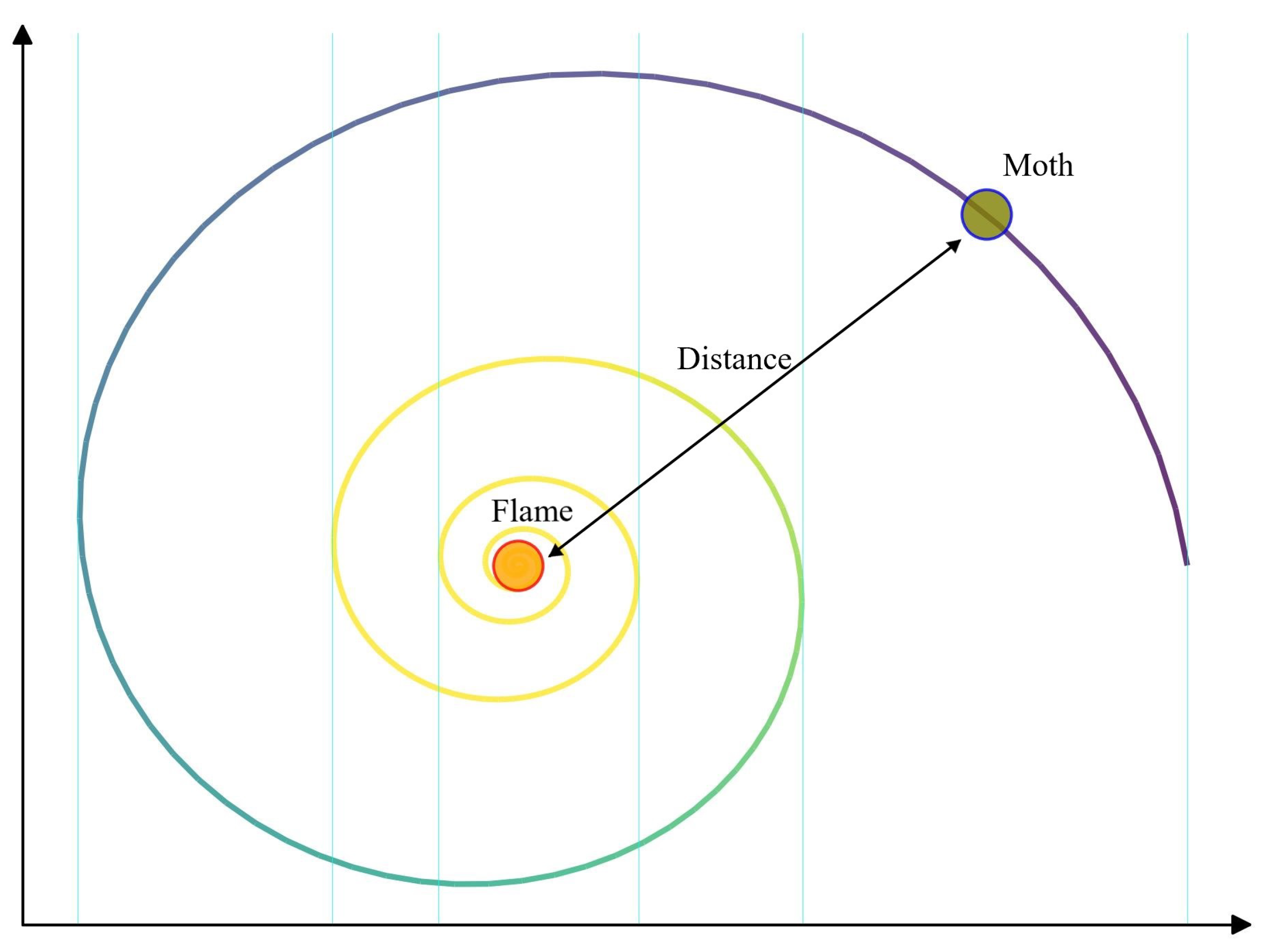
Figure 2.
Markov Decision Process framework showing state transitions, actions, and rewards

Figure 3.
Topological structure of the Three-feeder system.
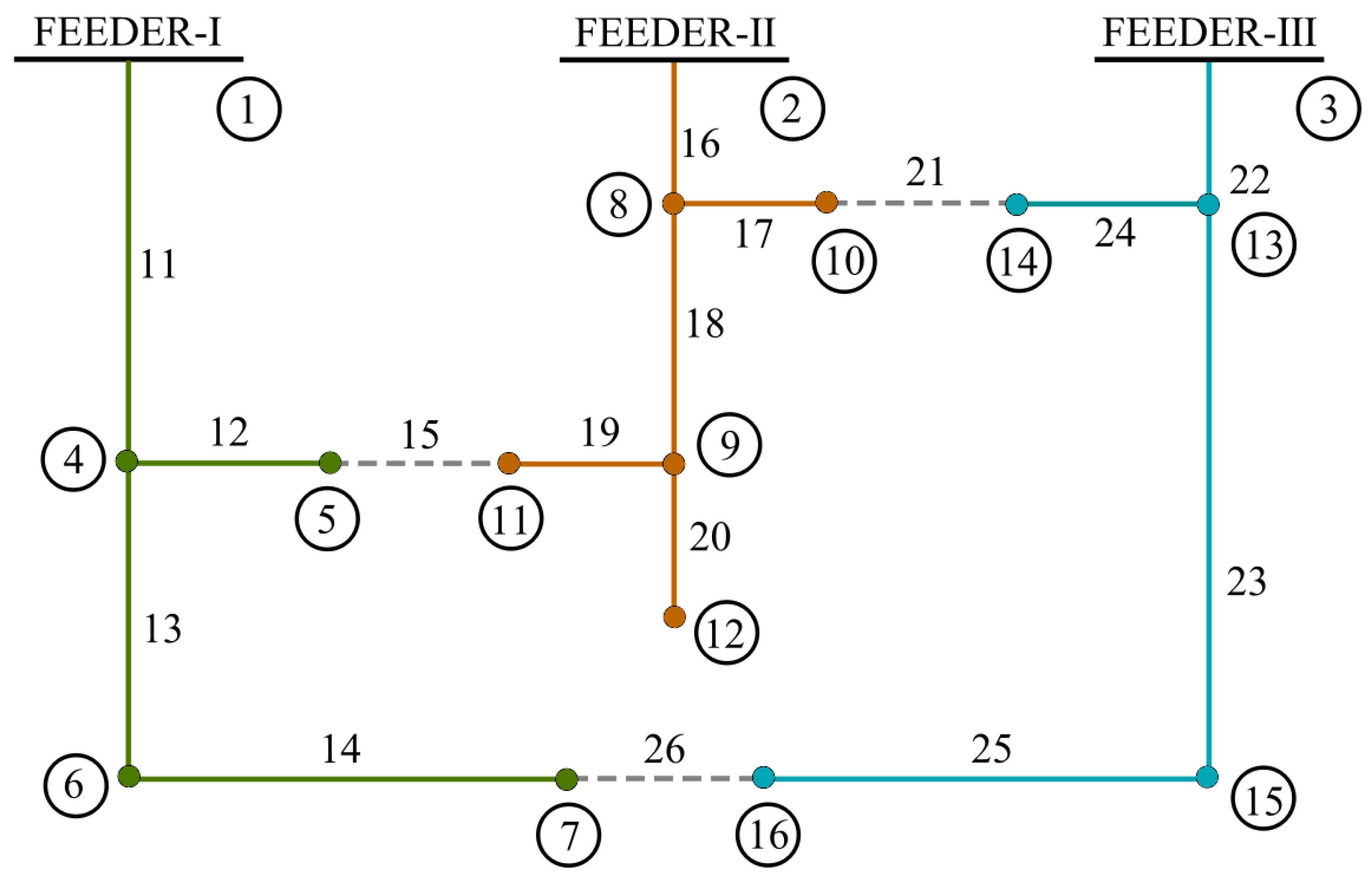
Figure 4.
Topological 6 applied in Case 2.
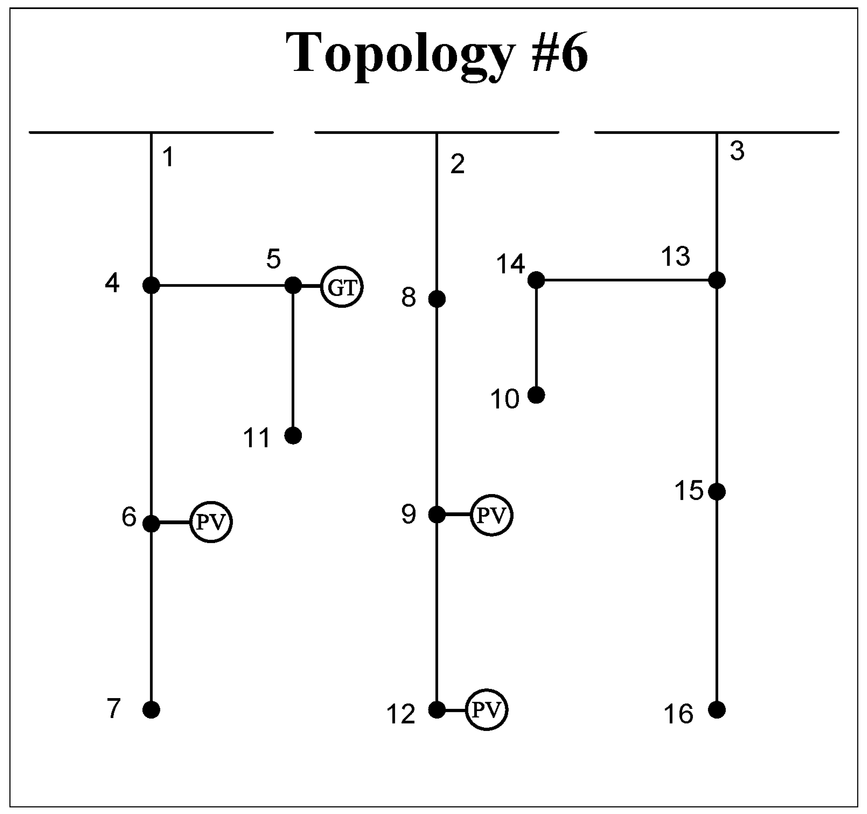
Figure 5.
Energy injection comparison of three cases.
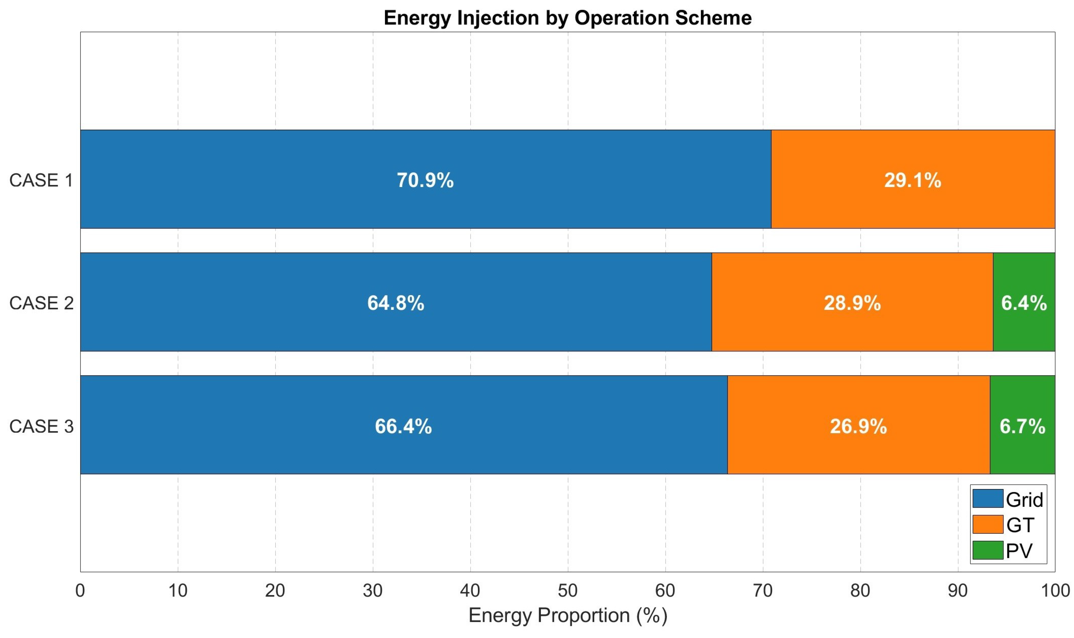

Table 1.
Cases Description.
| Gas Turbine | PV | Topology Reconfiguration | |
| Case 1 | Yes | No | No |
| Case 2 | Yes | Yes | No |
| Case 3 | Yes | Yes | Yes |
Table 2.
Comparison of Results from Different Cases.
| Power Loss/MW | Carbon Emission/t | Cost/million CNY | |
| Case 1 | 924.6459685 | 34059.67143 | 48.67017577 |
| Case 2 | 772.906651 | 31558.5414 | 44.78084034 |
| Case 3 | 480.8111423 | 30679.05149 | 43.8950143 |
Disclaimer/Publisher’s Note: The statements, opinions and data contained in all publications are solely those of the individual author(s) and contributor(s) and not of MDPI and/or the editor(s). MDPI and/or the editor(s) disclaim responsibility for any injury to people or property resulting from any ideas, methods, instructions or products referred to in the content. |
© 2025 by the authors. Licensee MDPI, Basel, Switzerland. This article is an open access article distributed under the terms and conditions of the Creative Commons Attribution (CC BY) license (http://creativecommons.org/licenses/by/4.0/).
Copyright: This open access article is published under a Creative Commons CC BY 4.0 license, which permit the free download, distribution, and reuse, provided that the author and preprint are cited in any reuse.


