Glioma Segmentation on 3D MRI Using 2D U-Net: A Study on the BraTS Dataset

1. Introduction

Brain tumors, particularly gliomas, are among the most aggressive and life-threatening cancers affecting the central nervous system [1]. Accurate and early delineation of tumor volumes from magnetic resonance imaging (MRI) scans is essential for effective treatment planning, including radiotherapy, surgical intervention, and prognosis assessment [2,3,4,5]. Manual annotation by radiologists, however, is time-consuming, subject to inter-observer variability, and not scalable for large datasets [6].

Segmentation methods in medical imaging are typically categorized into several classes, such as threshold-based techniques such as Otsu’s method [7], region-based approaches such as region growing [8], edge-based methods such as the Canny edge detector [9], clustering-based techniques such as K-means, Fuzzy C-Means [10], model-based methods such as active contours, level sets [11,12], and machine or deep learning-based approaches such as U-Net, Mask R-CNN, TransUNet [13,14,15]. Each category offers specific advantages depending on the imaging modality, anatomical target, and desired segmentation accuracy.

Although traditional segmentation techniques play a key role in outlining tumor boundaries, their accuracy can be significantly improved by incorporating advanced imaging methods. One such method, Diffusion Tensor Imaging (DTI), offers detailed insights into the brain’s white matter structure, helping to refine segmentation results and support more accurate tumor modeling [16,17].

Diffusion Tensor Imaging (DTI), a specialized MRI technique, is extensively used in neuroimaging to analyze the diffusion of water molecules, particularly for mapping white matter pathways. However, raw DTI images often suffer from low contrast and indistinct tissue boundaries. To enhance image quality, several methods have been employed, including the extraction of scalar indices such as fractional anisotropy (FA) and mean diffusivity (MD), bias field correction, and image fusion techniques. One notable method is the Uni-Stable enhancement technique, which combines clustering maps from various algorithms to produce stable, high-contrast images. Its three-dimensional extension, Uni-Stable-3D, interpolates between anisotropic slices to generate volumetric probability maps that are well-suited for robust tissue segmentation [18,19].

Beyond segmentation, tumor analysis also encompasses detection and prediction. Detection methods range from traditional techniques such as clustering and morphological operations to deep learning-based models, including U-Net, V-Net, and Mask R-CNN, which enable accurate tumor localization and delineation [20,21,22,23,24]. Prediction models aim to simulate tumor growth over time and include reaction-diffusion models, spatio-temporal simulations, and machine learning frameworks such as long short-term memory (LSTM) networks and survival analysis models. For example, an anisotropic reaction-diffusion model based on DTI data was proposed to simulate glioma progression across white and gray matter, demonstrating its effectiveness for treatment planning and prognosis [25].

This study addresses these limitations by proposing a deep learning-based approach for glioma segmentation using a 2D U-Net framework. The model is trained and tested on BraTS 3D multimodal MRI scans with expert-labeled tumor masks. Each scan includes four modalities: FLAIR, T1, T1CE, and T2. Though the data is 3D, our approach processes it as 2D slices to reduce computational demands while preserving relevant features. This allows efficient yet accurate tumor segmentation. Such models hold the potential to enhance diagnostic accuracy, reduce variability in interpretation, and accelerate clinical decision-making. Our solution is reproducible and based on widely available tools and datasets.

2. Dataset Description

In this study, we used the BraTS dataset, available on Synapse repository [26]. This dataset is widely recognized for benchmarking brain tumor segmentation algorithms and is composed of multimodal 3D MRI scans collected from patients diagnosed with glioblastoma multiforme (GBM) and low-grade gliomas (LGG). The dataset reflects clinical heterogeneity and variability in tumor appearance, making it suitable for training and evaluating deep learning models.

Each case in the dataset includes four different MRI scans, with each modality capturing distinct anatomical and pathological features. Together, they provide a comprehensive view of the brain, which helps improve the accuracy of tumor segmentation. An overview of these modalities is provided in Table 1.

Figure 1. Visual comparison of the four MRI modalities.

Figure 1. Visual comparison of the four MRI modalities.

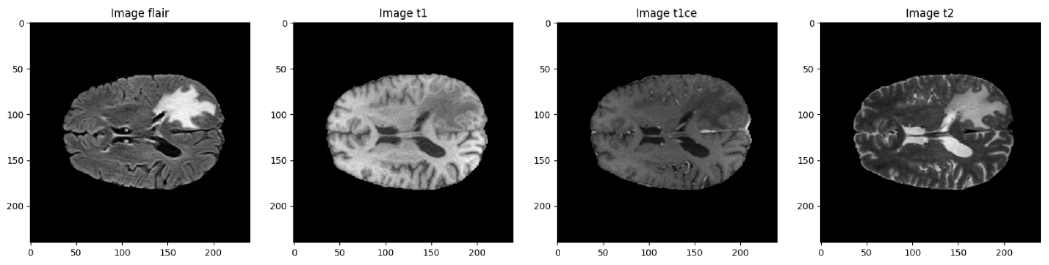
Table 1. Description of the four MRI modalities used in the dataset [26].

Modality	Description
T1	T1-weighted structural MRI
T1CE	T1-weighted with contrast enhancement (gadolinium)
T2	T2-weighted imaging, useful for fluid detection
FLAIR	Fluid-Attenuated Inversion Recovery, suppresses CSF to highlight lesions

Table 1. Description of the four MRI modalities used in the dataset [26].

Modality	Description
T1	T1-weighted structural MRI
T1CE	T1-weighted with contrast enhancement (gadolinium)
T2	T2-weighted imaging, useful for fluid detection
FLAIR	Fluid-Attenuated Inversion Recovery, suppresses CSF to highlight lesions

Each imaging modality offers distinct structural and pathological information, and combining them allows for a more precise mapping of tumor subregions. The dataset includes voxel-level annotations with four different classification labels.

Segmentation Labels:

The segmentation labels used in the dataset correspond to distinct tumor structures and are defined as follows

Table 2. Segmentation labels used in the dataset [26].

Label	Description
0	Background
1	Necrotic/Non-enhancing Tumor Core (NCR/NET)
2	Edema (ED)
4→3	Enhancing

Table 2. Segmentation labels used in the dataset [26].

Label	Description
0	Background
1	Necrotic/Non-enhancing Tumor Core (NCR/NET)
2	Edema (ED)
4→3	Enhancing

Sub-region combinations:

Additionally, these labels can be combined to form clinically meaningful tumor sub-regions

Table 3. Label combinations representing tumor sub-regions [26].

Label	Sub-region
1	Tumor Core (TC)
1, 2, 3	Whole Tumor (WT)
3	Enhancing Tumor (ET)

Table 3. Label combinations representing tumor sub-regions [26].

Label	Sub-region
1	Tumor Core (TC)
1, 2, 3	Whole Tumor (WT)
3	Enhancing Tumor (ET)

All images were manually segmented by four expert radiologists and validated by a board-certified neuroradiologist. The preprocessing steps included skull stripping, resampling to a 1 mm³ resolution, and co-registration [27].

3. Data and Image Preprocessing

In the field of medical imaging, especially when dealing with MRI scans, it's common to encounter differences in image intensity, spatial resolution, and anatomical alignment. These inconsistencies can pose significant challenges when training deep learning models, as they introduce noise and reduce data reliability. To address these issues, we implemented a thorough preprocessing pipeline aimed at normalizing the data, enhancing key features, and preparing both images and corresponding labels for segmentation. The process is organized into two main components: image preprocessing and label preprocessing.

3.1. Image Preprocessing

3.1.1. Intensity Normalization

MRI images often vary in brightness and contrast depending on the scanner type, imaging protocol, or even the patient being scanned. To reduce this variability and create a more consistent dataset, we applied normalization to each image. This technique standardizes the pixel intensity values so they center around a mean of zero with a standard deviation of one, helping the model better detect relevant structural patterns rather than being distracted by intensity differences [28].

3.1.2. Slice Selection

Rather than using the entire 3D volume, we focused on axial slices that are most relevant for tumor analysis. Specifically, slices from index 22 to 122 were extracted from each scan. This approach avoids slices that contain little to no brain tissue and ensures that the model concentrates on regions where tumors are typically found [3].

3.1.3. Cropping and Resizing

To ensure uniform input dimensions suitable for convolutional neural networks, each selected slice was cropped and resized to 128 × 128 pixels. This step helps maintain consistency across samples while also optimizing memory usage and training speed [29].

3.1.4. Data Augmentation

To make our model more robust and prevent overfitting, we incorporated several data augmentation techniques during training. These included random horizontal and vertical flips, small-angle rotations, and changes in image intensity. By simulating different imaging conditions, these augmentations help the model generalize better to new, unseen data [30].

3.1.5. Input Modalities

Each input sample was composed of two MRI sequences: FLAIR and T1CE. FLAIR images are particularly sensitive to areas of swelling or edema, while T1CE images are effective at showing regions of contrast uptake, often associated with active tumor tissue. Using both modalities together provided the model with richer and more complementary information for accurate tumor segmentation [25].

3.2. Label Preprocessing

Label Remapping

The original segmentation masks used four labels: 0, 1, 2, and 4. Since label 4 was not sequential (it represented the enhancing tumor), we remapped it to 3 to produce a clean, continuous label set. The final label scheme used in our study was:

Table 4. Label Remapping.

Label	Description
0	Background
1	Necrotic/Non-enhancing Tumor Core (NCR/NET)
2	Edema (ED)
3	Enhancing Tumor (ET)

Table 4. Label Remapping.

Label	Description
0	Background
1	Necrotic/Non-enhancing Tumor Core (NCR/NET)
2	Edema (ED)
3	Enhancing Tumor (ET)

This adjustment simplified data handling and ensured compatibility with standard categorical loss functions used in deep learning frameworks [32].

3.3. Model Architecture

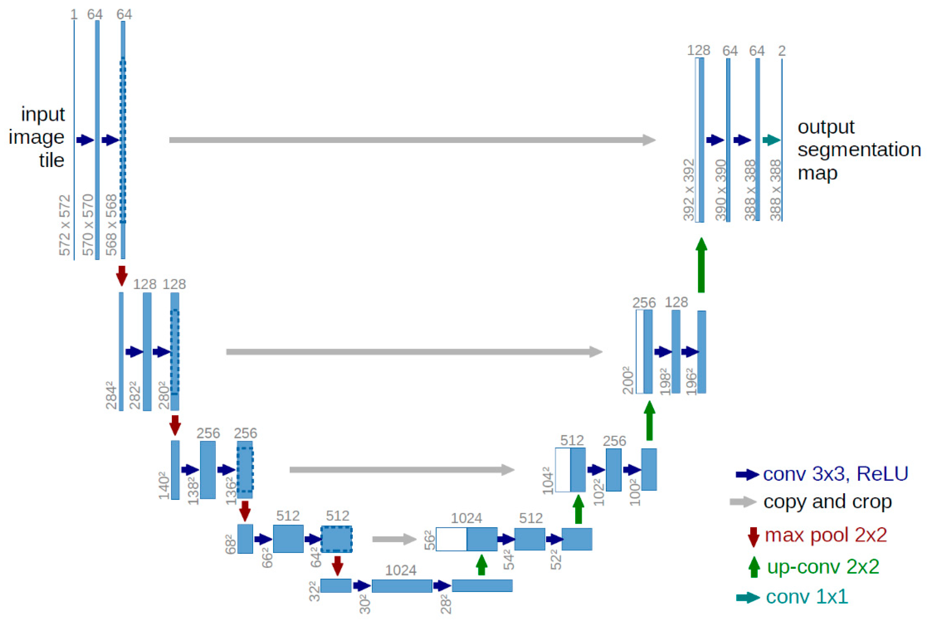
To perform brain tumor segmentation, we implemented a 2D U-Net architecture using TensorFlow 2.12 and Keras. U-Net is particularly effective for biomedical image segmentation, as it captures both local and global context while preserving spatial detail. Its encoder–decoder structure, enhanced with skip connections, allows for precise reconstruction of tumor boundaries by combining low-level spatial features with high-level semantic information [33].

3.3.1. U-Net Structure

• Encoder Path:

The encoder comprises four blocks. Each block includes two 2D convolutional layers (3×3 kernels, ReLU activation, 'same' padding), followed by a 2×2 max-pooling operation for downsampling. The number of filters doubles at each level: 32, 64, 128, and 256. This progressive structure enables the network to extract increasingly abstract features [33].

• Bottleneck:

At the network’s deepest layer, two convolutional layers with 512 filters each are followed by a dropout layer (rate = 0.2) to mitigate overfitting.

• Decoder Path:

The decoder mirrors the encoder with upsampling layers (via transposed convolutions), followed by convolutional blocks. Skip connections from corresponding encoder levels are concatenated to preserve spatial resolution. Filter sizes decrease symmetrically: 256, 128, 64, and 32.

• Output Layer:

The final layer is a 1×1 convolution with SoftMax activation, yielding a four-channel output that corresponds to the segmentation classes: background, necrotic core, edema, and enhancing tumor.

3.3.2. Input and Output Specifications

• Input Shape: Each input consists of two channels—FLAIR and T1CE—resulting in a shape of (128, 128, 2).
• Output Shape: The model produces a segmentation map of shape (128, 128, 4), with class-wise probabilities for each tumor sub-region.

Figure 2. U-NET Structure [34].

Figure 2. U-NET Structure [34].

3.3.3. Training Configuration

• Frameworks: TensorFlow 2.12 and Keras
• Loss Function: Categorical Crossentropy (suitable for multi-class segmentation)
• Optimizer: Adam optimizer with a learning rate of 0.001
• Regularization: Dropout (rate = 0.2) in the bottleneck layer

3.3.4. Evaluation Metrics

To comprehensively assess model performance, we used several evaluation metrics, each providing insights into different aspects of segmentation quality [35,36]:

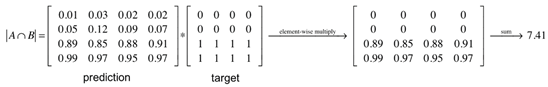
• Mean Intersection over Union (Mean IoU):

Also known as the Jaccard Index, this metric evaluates the overlap between predicted and ground truth regions by computing the ratio of their intersection to their union:

$$IoU={\displaystyle \frac{\left|A \cap B\right|}{\left|A \cup B\right|}}$$

(1)

It offers a strict measure of segmentation accuracy and is computed per class before averaging.

• Dice Similarity Coefficient (DSC):

The Dice coefficient measures how closely the predicted segmentation matches the ground truth. It is especially useful for imbalanced data such as tumor regions:

○

Overall Dice: Aggregates segmentation performance across all classes.

○

Class-specific Dice: Computed separately for necrotic core, edema, and enhancing tumor regions.

$$DSC={\displaystyle \frac{2 \left|A \cap B\right|}{\left(\left|A\right|+\left|B\right|\right)}}$$

(2)

• Precision:

Indicates the proportion of predicted positive pixels that are actually positive.

• Sensitivity (Recall):

Also called the true positive rate, this metric measures the model’s ability to detect all actual tumor pixels:

$$Sensitivity={\displaystyle \frac{TP}{\left(TP+FN\right)}}$$

(3)

• Specificity:

Measures the proportion of correctly identified negative (background) pixels, helping assess false positive rates:

$$Specificity={\displaystyle \frac{TN}{\left(TN+FP\right)}}$$

(4)

These metrics provide a balanced evaluation across detection accuracy, overlap, and class-specific segmentation—key for ensuring clinical reliability in automated tumor delineation systems.

3.4. Training Strategy

• Train/Val/Test split: 70% / 15% / 15%
• Epochs: 30
• Optimizer: Adam (learning rate = 0.001)
• Callbacks: ReduceLROnPlateau, EarlyStopping, CSVLogger
• Batch size: 1 (due to memory constraints)
• Custom DataGenerator for real-time augmentation and loading

4. Results

The U-Net model was trained for 30 epochs using TensorFlow and Keras. The best validation performance was observed at epoch 19, with the following results:

Table 5. Overall Validation Metrics and Additional Performance Measures.

Metric	Value
Validation loss	0.0284
Validation accuracy	98.84%
Global Dice Coefficient	0.5139
Precision	99.08%
Specificity	99.69%

Table 5. Overall Validation Metrics and Additional Performance Measures.

Metric	Value
Validation loss	0.0284
Validation accuracy	98.84%
Global Dice Coefficient	0.5139
Precision	99.08%
Specificity	99.69%

Table 6. Validation per-class Dice (epoch 19):.

Tumor Sub-Region	Validation Dice Score
Necrotic Core (NCR/NET)	0.4292
Edema (ED)	0.4644
Enhancing Tumor (ET)	0.5895

Table 6. Validation per-class Dice (epoch 19):.

Tumor Sub-Region	Validation Dice Score
Necrotic Core (NCR/NET)	0.4292
Edema (ED)	0.4644
Enhancing Tumor (ET)	0.5895

Training per-class Dice:

• NCR/NET: 0.4920
• ED: 0.6751
• ET: 0.6251

Table 7. Per-Class Dice Coefficients on the Training Set.

Tumor Sub-Region	Training Dice Score
Necrotic Core (NCR/NET)	0.4920
Edema (ED)	0.6751
Enhancing Tumor (ET)	0.6251

Table 7. Per-Class Dice Coefficients on the Training Set.

Tumor Sub-Region	Training Dice Score
Necrotic Core (NCR/NET)	0.4920
Edema (ED)	0.6751
Enhancing Tumor (ET)	0.6251

Minor overfitting was observed after epoch 19.

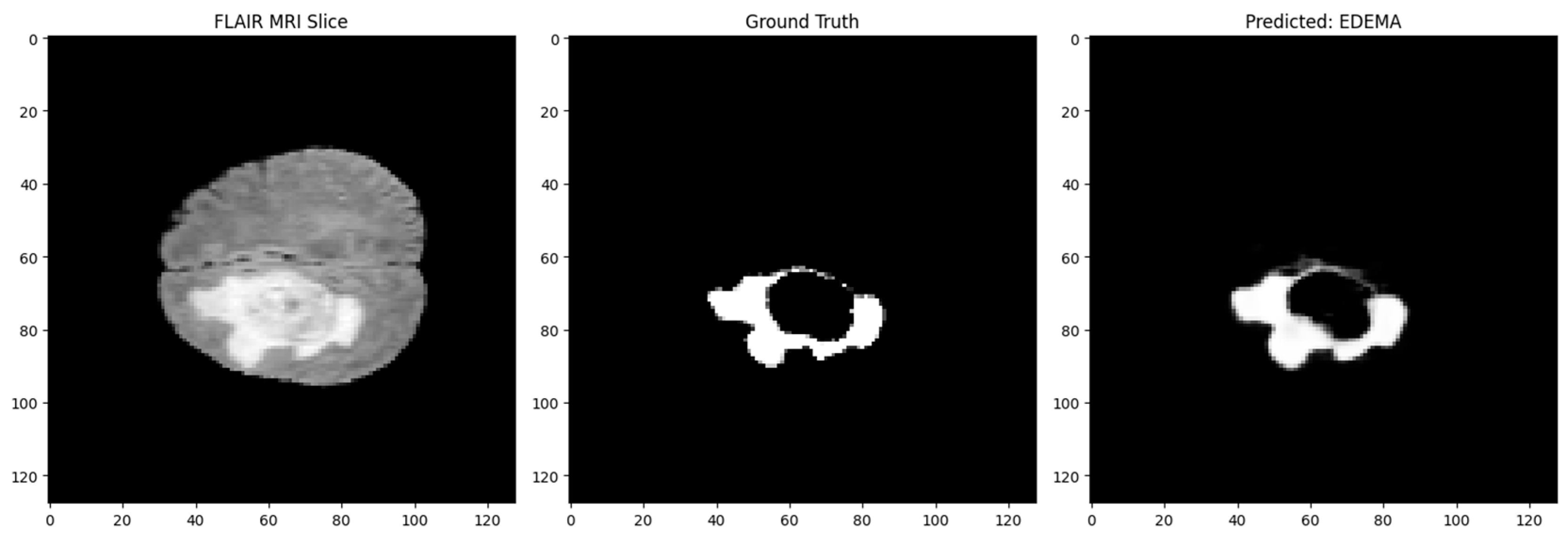
Figure 3. Segmentation: Input MRI, Ground Truth, and Prediction.

Figure 3. Segmentation: Input MRI, Ground Truth, and Prediction.

5. Discussion

The results of this work show that employing a 2D U-Net for brain tumor segmentation—by processing 3D MRI scans slice by slice—is a practical and effective strategy. Although this method doesn't leverage the complete 3D spatial context, it still performed well in identifying critical tumor regions like the Whole Tumor (WT), Tumor Core (TC), and Enhancing Tumor (ET). This aligns with earlier findings from BraTS evaluations that showed 2D models can still provide reliable results when properly trained [37].

5.1. Performance Observations

The model showed stronger accuracy on larger and more consistent tumor components, such as the whole tumor and tumor core. However, segmenting the enhancing tumor region proved more difficult. This subregion often presents with irregular shapes and smaller volume, which tends to challenge even the best segmentation models—a limitation highlighted in various segmentation studies [38].

5.2. Model Advantages

The U-Net’s encoder–decoder framework, along with its skip connections, proved highly beneficial for preserving fine spatial details while also capturing contextual information at multiple levels. This structure, originally designed for biomedical tasks, supports precise boundary delineation even with limited training data [33].Furthermore, regularization techniques like dropout, combined with data augmentation strategies such as flipping and intensity shifts, helped improve the model’s generalization by reducing overfitting risk [39].

6. Conclusions

This thesis supports the effectiveness of a 2D U-Net model for segmenting brain tumors from multimodal MRI data. Even without utilizing full volumetric information, the model successfully distinguished between key tumor components and achieved encouraging segmentation performance.

The main benefit of this approach lies in its simplicity and efficiency. It doesn’t require extensive computational resources, making it accessible for both clinical research settings and practical deployment. The findings reinforce the potential of 2D convolutional models in medical image segmentation, especially when paired with thoughtful preprocessing and training strategies [40].

References

- Stupp, W.; et al. Radiotherapy plus concomitant and adjuvant temozolomide for glioblastoma. New England Journal of Medicine 2005, 352, 987–996. [Google Scholar] [CrossRef] [PubMed]
- Bauer, S.; Wiest, R.; Nolte, L.-P.; Reyes, M. A survey of MRI-based medical image analysis for brain tumor studies. Physics in Medicine and Biology 2013, 58, R97–R129. [Google Scholar] [CrossRef] [PubMed]
- Menze, B.H.; Jakab, A.; Bauer, S.; Kalpathy-Cramer, J.; Farahani, K.; Kirby, J.; et al. The Multimodal Brain Tumor Image Segmentation Benchmark (BRATS). IEEE Transactions on Medical Imaging 2015, 34, 1993–2024. [Google Scholar] [CrossRef] [PubMed]
- Baid, U.; et al. The RSNA-ASNR-MICCAI BraTS 2021 Benchmark on Brain Tumor Segmentation and Radiogenomic Classification. arXiv 2021, arXiv:2107.02314. [Google Scholar]
- Bakas, S.; Akbari, H.; Sotiras, A.; Bilello, M.; Rozycki, M.; Kirby, J.S.; et al. Advancing The Cancer Genome Atlas glioma MRI collections with expert segmentation labels and radiomic features. Nature Scientific Data 2017, 4, 170117. [Google Scholar] [CrossRef] [PubMed]
- Havaei, M.; et al. Brain tumor segmentation with deep neural networks. Medical Image Analysis 2017, 35, 18–31. [Google Scholar] [CrossRef] [PubMed]
- Otsu, N. A threshold selection method from gray-level histograms. IEEE Transactions on Systems, Man, and Cybernetics 1979, 9, 62–66. [Google Scholar] [CrossRef]
- Adams, R.; Bischof, L. Seeded region growing. IEEE Transactions on Pattern Analysis and Machine Intelligence 1994, 16, 641–647. [Google Scholar] [CrossRef]
- Canny, J. A computational approach to edge detection. IEEE Transactions on Pattern Analysis and Machine Intelligence 1986, 8, 679–698. [Google Scholar] [CrossRef] [PubMed]
- Bezdek, J.C.; Ehrlich, R.; Full, W. FCM: The fuzzy c-means clustering algorithm. Computers & Geosciences 1984, 10, 191–203. [Google Scholar] [CrossRef]
- Kass, M.; Witkin, A.; Terzopoulos, D. Snakes: Active contour models. International Journal of Computer Vision 1988, 1, 321–331. [Google Scholar] [CrossRef]
- Osher, S.; Sethian, J.A. Fronts propagating with curvature-dependent speed: Algorithms based on Hamilton–Jacobi formulations. Journal of Computational Physics 1988, 79, 12–49. [Google Scholar] [CrossRef]
- Ronneberger, O.; Fischer, P.; Brox, T. U-Net: Convolutional networks for biomedical image segmentation. In Proc. Medical Image Computing and Computer-Assisted Intervention (MICCAI); 2015; pp. 234–241. [Google Scholar]
- He, K.; Gkioxari, G.; Dollár, P.; Girshick, R. Mask R-CNN. In Proc. IEEE International Conference on Computer Vision (ICCV); 2017; pp. 2961–2969. [Google Scholar]
- Chen, J.; et al. TransUNet: Transformers make strong encoders for medical image segmentation. arXiv 2021. [Google Scholar] [CrossRef]
- Elaff, I.; EL-Kemany, A.; Kholif, M. Universal and stable medical image generation for tissue segmentation (The unistable method). Turkish Journal of Electrical Engineering and Computer Sciences 2017, 25, 32. [Google Scholar] [CrossRef]
- Elaff, I. Medical Image Enhancement Based on Volumetric Tissue Segmentation Fusion (Uni-Stable 3D Method). Journal of Science, Technology and Engineering Research 2023, 4, 78–89. [Google Scholar] [CrossRef]
- Elaff, I. Brain Tissue Classification Based on Diffusion Tensor Imaging: A Comparative Study Between Some Clustering Algorithms and Their Effect on Different Diffusion Tensor Imaging Scalar Indices. Iran J Radiol. 2016, 13, e23726. [Google Scholar] [CrossRef] [PubMed]
- El-Aff, I. Human brain tissues segmentation based on DTI data. In Proceedings of the 2012 11th International Conference on Information Science, Signal Processing and their Applications (ISSPA), Montreal, QC, Canada; 2012; pp. 876–881. [Google Scholar] [CrossRef]
- El-Dahshan, E.-S.A.; Hosny, T.; Salem, A.-B.M. Hybrid intelligent techniques for MRI brain images classification. Digital Signal Processing 2010, 20, 433–441. [Google Scholar] [CrossRef]
- Kapur, T.; Grimson, W.E.L.; Wells, W.M.; Kikinis, R. Segmentation of brain tissue from magnetic resonance images. Medical Image Analysis 1996, 1, 109–127. [Google Scholar] [CrossRef] [PubMed]
- Ronneberger, O.; Fischer, P.; Brox, T. U-Net: Convolutional networks for biomedical image segmentation. In MICCAI; Springer, 2015; pp. 234–241. [Google Scholar]
- Milletari, F.; Navab, N.; Ahmadi, S.A. V-Net: Fully convolutional neural networks for volumetric medical image segmentation. In 3DV; IEEE, 2016; pp. 565–571. [Google Scholar]
- Jiang, Z.; Zhang, H.; Wang, Y.; Ko, H. Mask R-CNN with DenseNet for brain tumor segmentation. Computers, Materials & Continua 2021, 67, 1941–1955. [Google Scholar]
- Elaff, I. Comparative study between spatio-temporal models for brain tumor growth. Biochemical and Biophysical Research Communications 2018, 496, 1263–1268. [Google Scholar] [CrossRef] [PubMed]
- The BraTS Consortium. BraTS: Brain Tumor Segmentation dataset. The Cancer Imaging Archive. Available online: https://www.synapse.org/#!Synapse:syn36640318.
- CBICA/Upenn. BraTS: Brain Tumor Segmentation dataset. Synapse. 2023. Available online: https://www.synapse.org/#!Synapse:syn51156910/wiki/622351.
- Nyúl, L.G.; Udupa, J.K.; Zhang, X. New variants of a method of MRI scale standardization. IEEE Transactions on Medical Imaging 2000, 19, 143–150. [Google Scholar] [CrossRef] [PubMed]
- Isensee, F.; Petersen, J.; Kohl, S.; Jäger, P.F.; Maier-Hein, K.H. nnU-Net: A self-configuring method for deep learning-based biomedical image segmentation. Nature Methods 2021, 18, 203–211. [Google Scholar] [CrossRef] [PubMed]
- Shorten, C.; Khoshgoftaar, T.M. A survey on image data augmentation for deep learning. Journal of Big Data 2019, 6, 60. [Google Scholar] [CrossRef]
- Bakas, S.; Reyes, M.; Jakab, A.; Bauer, S.; Rempfler, M.; Crimi, A.; Menze, B.H. Identifying the best machine learning algorithms for brain tumor segmentation, progression assessment, and overall survival prediction in the BRATS challenge. arXiv 2018. [Google Scholar] [CrossRef]
- Havaei, M.; Davy, A.; Warde-Farley, D.; Biard, A.; Courville, A.; Bengio, Y.; Larochelle, H. Brain tumor segmentation with deep neural networks. Medical Image Analysis 2017, 35, 18–31. [Google Scholar] [CrossRef] [PubMed]
- Ronneberger, O.; Fischer, P.; Brox, T. U-Net: Convolutional Networks for Biomedical Image Segmentation. In Medical Image Computing and Computer-Assisted Intervention (MICCAI); 2015; pp. 234–241. [Google Scholar]
- Ronneberger, O.; Fischer, P.; Brox, T. U-Net: Convolutional Networks for Biomedical Image Segmentation. Proc. MICCAI 2015, 9351, 234–241. [Google Scholar]
- Taha, A.A.; Hanbury, A. Metrics for evaluating 3D medical image segmentation: Analysis, selection, and tool. BMC Medical Imaging 2015, 15, 1–28. [Google Scholar] [CrossRef] [PubMed]
- Zou, K.H.; et al. Statistical validation of image segmentation quality based on a spatial overlap index: Scientific reports. Academic Radiology 2004, 11, 178–189. [Google Scholar] [CrossRef] [PubMed]
- Bakas, S.; et al. Identifying the best machine learning algorithms for brain tumor segmentation, progression assessment, and overall survival prediction in the BRATS challenge. Medical Image Analysis 2018, 55, 115–142. [Google Scholar]
- Isensee, F.; et al. Nnu-net: Self-adapting framework for U-Net-based medical image segmentation. Nature Methods 2021, 18, 203–211. [Google Scholar] [CrossRef] [PubMed]
- Shorten, C.; Khoshgoftaar, T.M. A survey on image data augmentation for deep learning. Journal of Big Data 2019, 6, 1–48. [Google Scholar] [CrossRef]
- Zhou, Z.; et al. UNet++: A nested U-Net architecture for medical image segmentation. Deep Learning in Medical Image Analysis and Multimodal Learning for Clinical Decision Support 2018, 3–11. [Google Scholar]
Disclaimer/Publisher’s Note: The statements, opinions and data contained in all publications are solely those of the individual author(s) and contributor(s) and not of MDPI and/or the editor(s). MDPI and/or the editor(s) disclaim responsibility for any injury to people or property resulting from any ideas, methods, instructions or products referred to in the content. |
© 2025 by the authors. Licensee MDPI, Basel, Switzerland. This article is an open access article distributed under the terms and conditions of the Creative Commons Attribution (CC BY) license (http://creativecommons.org/licenses/by/4.0/).
Copyright: This open access article is published under a Creative Commons CC BY 4.0 license, which permit the free download, distribution, and reuse, provided that the author and preprint are cited in any reuse.