
Submitted:
23 June 2025
Posted:
24 June 2025
You are already at the latest version
Abstract
The recent losses and damages due to climate change have destabilized the insurance industry. As global warming is one of the most critical aspects of climate change, it is essential to investigate the extent to which greenhouse gas emissions affect the financial stability of insurers. Insurers do not typically emit substantial greenhouse gases directly, while their underwriting and investment activities play a substantial role in enabling companies that do. This article uses panel data regressions to analyze companies in all segments of insurance and from all geographic regions in the world from 2004 to 2023. The main finding is that insurers who increase their greenhouse gas emissions become financially unstable. This result is consistent across all three scopes (scope 1, scope 2, and scope 3) of emissions. Furthermore, the findings reveal that this impact is related to reserves and reinsurance. Specifically, reserves increase with greenhouse gas emissions, while premiums ceded to reinsurers decline. Thus, high-polluting insurers retain a significant share of carbon risk, eventually becoming financially weak. The results encourage several policy recommendations, highlighting the need for instruments that improve the assessment and disclosure of insurers’ carbon footprints. This is crucial to achieving environmental targets and enhancing the stability of both the insurance market and the economic system.
Keywords:
greenhouse gas emissions
; insurance companies
; financial stability
; reserves
; reinsurance
Abstract
1. Introduction
Global warming and climate change are destabilizing the insurance industry. Regulators and environmental authorities recognize that, despite mitigation and adaptation efforts, the more recent (economic and non-economic) “loss and damage” due to climate change have been substantial (United Nations Environment Programme, 2023). Therefore, insurers have to face huge payouts, threatening the solvency of their businesses. Examining the responses activated by United States insurers to environmental risks, Gupta et al. (2023) show that many firms remain inadequately prepared for climate change risks, exhibiting a relatively high level of financial weakness. The Bank for International Settlements (BIS) warns that there is a chance that the global average temperature increase target under the Paris Agreement could be breached, pushing the world, the global economy and financial systems into uncharted territory (Khoo and Yong, 2023). For underwriters, this could increase the difficulty to measure, predict and apportion risks. Insurers recognize that, when their own emissions grow or when they underwrite carbon-intensive businesses, they are supporting unsustainable business practices (KPMG, 2023), which in the longer term would make their operations unfeasible.
The recent floods and extreme weather events in the United States have been blamed for fueling a crisis in the insurance market. As a result, insurance premiums have climbed, and some insurance companies have started to refuse to insure real estate (BBC, 2024). Evidently, the carbon footprint of insurers has an impact on their financial conditions, affecting the sustainability of the risk- sharing services that insurance provides. In turn, this has profound implications on the stability of the insurance market and the entire economic system. To the best of our knowledge, this is the first study to investigate empirically how the financial stability of insurers is related to their scope 1, scope 2, and scope 3 emissions, outlining potential channels that determine this link. Addressing this topic is important to extend the knowledge about the impact of greenhouse gas emissions on insurance operations, which the current literature has investigated looking at, for example, corporate valuation, performance, and capital costs. Even more importantly, the findings deliver insights for policy making, supporting the need for rules and initiatives aimed at reducing carbon exposures within the insurance sector, to eventually enhance the health of the economic system, beyond benefiting the environment. The article is organized as follows. Section 2 reviews the
2. Literature and Development of Hypotheses
Emissions of CO2 and nonCO2 are the major causes of global warming (Montzka et al., 2011), which is one of the main aspects of climate change (NASA, 2024). The impact of greenhouse gas emissions on corporate financial decisions is multifaceted. Research has proved that carbon risk affects corporations from different perspectives, ranging from corporate equity performance (Oestreich and Tsiakas, 2015; Wen et al., 2020; Bolton and Kacperczyk, 2021, 2024), valuation (Matsumura et al., 2014; Clarkson et al., 2015; Griffin et al., 2017; H´agen and Ahmed, 2024), investor decision-making (Krueger et al., 2020), to capital costs (Kim et al., 2015; Bui et al., 2020). With the growing attention in the economy to environmental topics, a key issue for both cor- porate managers and policy makers has become to understand whether the carbon footprint of businesses can make them financially unstable. For example, Kabir et al. (2021) analyse carbon emissions of non-financial firms worldwide, reporting that increasing emissions lead to a higher default risk. This is mainly due to corporate emissions having a negative effect on corporate cash flow volatility and profitability. Based on the S&P 500 index members, Perera et al. (2023) find that firms’ carbon emissions intensity leads to a higher idiosyncratic volatility. Concerning the banking sector, Chabot and Bertrand (2023) develop a theoretical framework for the transmission of climate risks to financial institutions and the financial system. To test the model predictions, the authors use a panel of European financial institutions. They show that transition climate risk, measured by greenhouse gas emissions (scope 1, scope 2, and scope 3), negatively affects financial stability at both the institutional and system-wide levels.
As insurers play a pivotal role in addressing environmental challenges throughout the whole economy, exposure to carbon risk may bring instability within the insurance industry. Dlugolecki (2008) argues that global warming has several implications on underwriters: “Catastrophe models are wrongly calibrated; premiums are too low; exposures are too high; claim-handling capacity is inadequate; and credit ratings are too generous.” Recent evidence illustrates substantial losses and damages to property and life due to natural catastrophes, resulting in huge payouts that, in turn, threaten the solvency of many businesses. Insurers recognize that, by underwriting carbon-intensive businesses, they are supporting unsustainable business practices (KPMG, 2023). Therefore, given their pivotal role in the net-zero transition, insurers are currently struggling to manage their carbon footprints to avoid carrying the negative consequences related to climate change risks.
The stability of insurance operations is affected by climate change risks both in the short-term and in the long-term (KPMG, 2022). The increasing frequency and severity of natural disasters and extreme weather events make more difficult for insurers to predict losses and appropriately price insurance claims. The unstable business implies also troubles in the affordability and availability of insurance (European Insurance and Occupational Pensions Authority, 2023). The Bank of England points out that the stability of insurers, as financial intermediaries, is threatened by climate risks in the form of physical, transition, while also of “liability risk”, which is directly related to investment provision and insurance services (Bank of England, 2019).
While carbon emissions seem to impact the insurer’s stability, the literature has not examined the drivers of this effect. Both reserves and reinsurance can be relevant for this mechanism. In fact, the uncertainty related to climate change affects the ability to establish adequate levels of reserves, making it more difficult for insurers to quantify the likelihood and size of the influence that climate change has on both their own operations and the operations of their customers. Therefore, carbon exposure would lead to higher reserve levels that are arguably necessary to cover possible volatility in future payouts. However, if insurers react to the frequent and increasingly serious nature of environmentally destructive events by continually increasing premiums and reserves, they may impair their underwriting capacity and profitability — a solution that, in the longer term, would be unfeasible and bring instability.
Reinsurance plays a key role in helping insurance companies to pay for large unexpected losses caused by natural disasters. However, the high frequency of extreme weather events has led rein- surers to receive many claims. A recent report from the rating agency Fitch Ratings points out that the incidence of climate losses has prompted reinsurers to step back, as the reinsurance industry has become more averse to backstopping “secondary perils,” which are smaller but more frequent extreme weather events (Fitch Ratings, 2024). Another rating agency, S&P, said that ”more than half of the top 20 global reinsurers maintained or reduced their natural catastrophe exposures during the January 2023 renewals, despite the improved pricing terms and conditions and rising demand” (S&P, 2023). Thus, increasing carbon risk exposure would decrease the availability of reinsurance. In other words, high polluting insurers would end up retaining a larger share of the risk.
Despite the concerns raised among policy makers and practitioners in the insurance industry about carbon footprints, the existing research presents a gap in providing evidence related to insurers’ stability. This article aims to explore this issue. The main argument is that greenhouse gas emissions expose insurers to environmental risks, which ultimately make the firms financially unstable. This effect concerns both direct and indirect emissions, measured by scope 1, scope 2, and scope 3 emissions. Arguably, both reserves and reinsurance are two important drivers for this impact. Overall, the following working hypotheses will be tested in the next section using panel data analyses:
HP1:
Insurers’ carbon emissions make insurance firms financially unstable.
HP2
: Scope 1, scope 2, and scope 3 emissions reduce insurance firms’ stability similarly.
HP3
: Increasing greenhouse gas emissions make insurers financially unstable through growing reserves.
HP4
: Increasing greenhouse gas emissions make insurers financially unstable through decreasing reinsurance.
3. Methods
The data-source for this analysis is SP Capital IQ, which provides data on carbon emissions as well as accounting data for worldwide insurers. The companies are all publicly listed and operate in one of the following segments of insurance: Financial guarantee, life and health, managed care, mortgage guarantee, multiline, property and casualty, and title insurance. Based on these screening criteria, the final sample consists of 2,043 firm-year observations from 2004 to 2023. The sample composition by segments of insurance is displayed in Table 1.
According to the GHG Protocol Corporate Standard, a company should separately account for and report its greenhouse gs emissions into three “scopes”. Scope 1 emissions are direct greenhouse gas emissions that occur from sources that are owned or controlled by the company. Scope 2 covers indirect emissions from the
purchase and use of electricity, steam, heating and cooling. Scope 3 includes all other indirect
emissions that occur in the upstream and downstream activities of an organization (Partnership for Carbon Accounting Financials, 2022). The emissions associated with investment and insurance activity are defined as scope 3 emissions, and are known as financed or insurance-associated emissions (KPMG, 2023)
For each scope, the total annual values (in tonnes CO2e) of greenhouse gas emissions are ob-
tained. The data-source provides the figures combining companies’ reported data and modeled data. Modeled data are computed using process-based approaches and multi-sector Environmentally- Extended Input-Output (EEIO) modeling.[1] In the analysis, the natural log of the scope 1, 2, and 3 emission values are indicated respectively with GHG1, GHG2, and GHG3.[2]
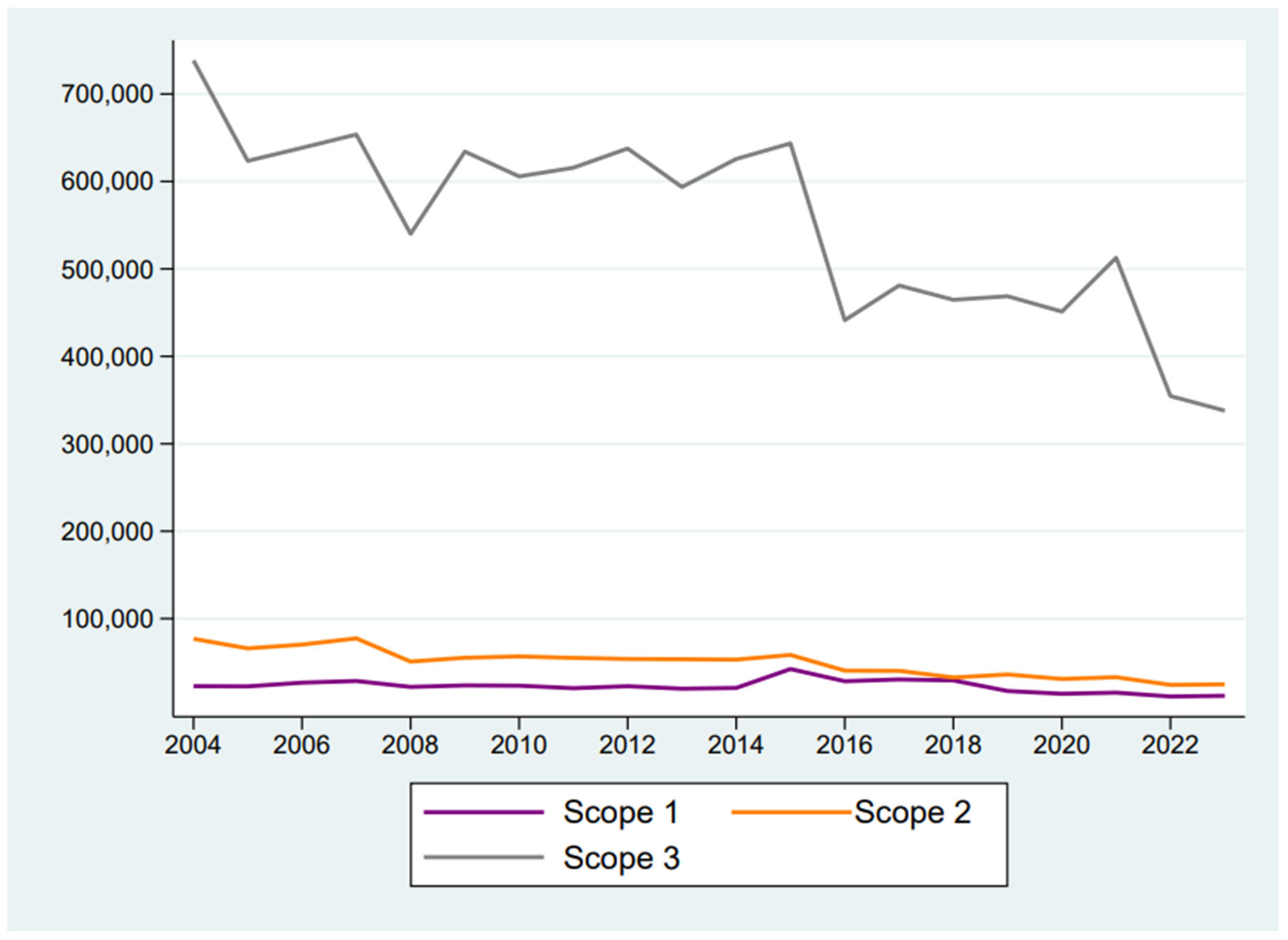
Figure 1 shows
the averages of insurers’ greenhouse gas emissions over years. Despite
a decreas- ing trend over time, the figure highlights how scope 3 greenhouse gas emissions widely overcome
scope 1 and scope 2 emissions. A similar pattern concerning the magnitude
of scope 1, scope 2, and scope 3 emissions concerns also banks,
has it has been outlined by Bressan (2025).
This pattern depends from the business model of insurers, which, in
fact, are ”unique in the need to consider both
investment and insurance emissions” (KPMG, 2023).
In 2020 the reporting finance
portfolio emissions of European
insurers were ”over 700 times larger than direct emissions” (Deloitte, 2023). More recently, it has been calculated that,
across the insurance industry worldwide, more than 95 percent of emissions fall into Scope 3
(KPMG, 2023).
Figure 1.
Greenhouse gas emissions (tonnes CO2e) of insurance companies during 2004-2023.
The financial stability of insurers is measured using two alternative measures. The first measure is the combined ratio (CR), i.e. the sum of incurred losses, loss adjustment expenses plus other underwriting expenses, divided by earned premiums (Rejda, 2005). A combined ratio below 100% indicates that the company is making an underwriting profit, whereas a ratio above 100% suggests an underwriting loss. Doherty and Garven (1995) provide theoretical evidence for the negative
relationship between the combined ratio and the solvency rate of a corporation. In empirical research, the combined ratio is employed to examine insurers’ financial conditions. For example, Browne and Hoyt (1995) report that a ratio could indicate unfavorable underwriting results and lower profitability. Chen and Wong (2004) use the combined ratio to study the main determinants of insurers’ financial health. Bressan and Du (2024b) employ the combined ratio to show that, by purchasing reinsurance, insurers become financially more solid. Regulators closely monitor insurers’ combined ratios to ensure that they maintain a sufficient level of capital to cover claims while also operating sustainably. From a regulatory standpoint, a persistently high combined ratio can trigger increased scrutiny and potential intervention to safeguard the insurer’s solvency and the interests of the insured. For example, in the European framework, the European Insurance and Occupational Pensions Authority (EIOPA) uses the combined ratio to report on insurers’ solvency and profitability (European Insurance and Occupational Pensions Authority, 2025).
The second measure assessing the financial stability of insurance companies is the underwriting leverage, or premium-to-surplus ratio, i.e. the ratio of net premiums written to policyholder surplus (PS). The policyholder surplus is the total assets net of any liabilities, and it represents the amount of money that the firm has left over after paying its claims and other expenses. The premium- to-surplus ratio, which is sometimes referred as the “insurance exposure”, has been advocated on occasion as a rule-of-thumb indicator of insolvency (Lai, 2006). Leng and Meier (2006) examine underwriting cycles, using the premium-to-surplus ratio to measure insurers’ risk taking behavior. In fact, a high ratio indicates that an insurer has a high level of risk exposure compared to its surplus, which could result in financial difficulties if it experiences a significant loss. On the other hand, a lower ratio depicts greater financial strength for the company. As a rule, regulators set up less than 3-to-1 premium-to-surplus ratio to be adhered by insurance companies to remain rela- tively healthy. In the Unite States, the premium-to-surplus ratio is employed within the Insurance Regulatory Information System (IRIS) to predict insurers’ financial strength and assess insolvency risk (National Association of Insurance Commissioners, 2023). The premium-to-surplus ratio is also used by rating agencies to evaluate an insurer’s financial profile and assign credit ratings.
The working hypotheses 3 and 4 regard effects on reserves and reinsurance. The measure for reserves (RES) is the ratio of reserves to policyholder surplus (National Association of Insurance Commissioners, 2023). This quantity denotes the amount that the firm has set aside for potential
claims compared to the total assets it possesses (minus its liabilities), and is inversely related to the insurer’s capability to effectively serve its clients. In fact, a high RES signals that the firm might need to pay a higher amount in losses compared to what it could potentially sell to raise cash. The measure of reinsurance (REINS) is the ratio of ceded premiums to gross premiums (Bressan and Du, 2024b). Ceded premiums are the premiums that an insurer pays to another company (the reinsurer) to cover a portion of its liabilities, while gross premiums are the total premium an insurance company receives from its policyholders. A high REINS indicates that the insurer transfers a large portion of its premium to a reinsurer to mitigate its risk exposure, thereby ensuring financial stability.
The regression models control for additional firm-specific aspects. These include financial lever- age, measured with the ratio of debt to total assets (DEBT ), and profitability, assessed with the return-on-assets (ROA), i.e. the ratio of net income to total assets. Additionally, the ratio of gross premiums to assets (GP ) controls for the underwriting business, while the ratio of investment in- come to assets (INV ) captures to what extent the firm generates income by investing policyholder funds in various assets, so to earn returns through interest, dividends, and capital appreciation.
The definition of the variables is summarized in Table 2. After winsorizing the variables at the 1st and 99th percentiles, descriptive statistics and pair-wise correlation coefficients are reported, respectively, in Table 3 and Table 4.
The estimation period is 2004–2023, except for ESG which is available in the period 2013–2023. Table 2 defines the variables.
In order to develop a first insight on the relationship between greenhouse gas emissions and financial characteristics of insurers, in Table 5 the averages of the variables are calculated for sub-samples of low/medium/high polluting firms. The sub-samples are defined every year using the sample distribution. Namely, high polluting insurers have GHG3 above or equal the 90th percentile, medium polluting insurers have GHG3 between the 30th and the 90th percentile, while low polluting insurers have GHG3 below or equal the 30th percentile. The numbers reveal that high polluting insurers are financially weaker (HP1), as the combined ratio and the premium-to-surplus ratio are respectively 9% and 62% higher than within low polluting insurers. Moreover, reserves are considerably higher within high polluting firms (HP3), while the insurance purchased is lower (HP4). Based on the Dunn’s test (Dunn, 1964), all these differences are statistically significant at the 1% level of significance. Similar comparisons across the three sub-samples are found also when the firms are classified according to the distribution of GHG1 and GHG2. However, for brevity, these outcomes are omitted, while remaining available upon request.
The estimation period is 2004–2023. Table 2 defines the variables. The Dunn’s test (Dunn, 1964) performs pairwise comparisons between firms with low and high emissions. The statistics has a chi-squared distribution. *, **, and *** indicate significance at the 10%, 5%, and 1% level, respectively.
To test the working hypotheses HP1 and HP2 more formally, the following equation estimates the effect on the financial stability of bank j in year t from its greenhouse gas emissions:
Financial stabilityf,j,t = α + β GHGs,j,t + γControlsj,t + Fixed effects + ϵj,t
The subscript f stays for, alternatively, the combined ratio (CR) and the premium-to-surplus ratio (PS). The subscript s denotes the emissions’ scope, as the model is tested separately for GHG1, GHG2, and GHG3. The set of control variables includes DEBT , ROA, GP , and INV . Fixed effects capture characteristics that are invariant through time and geographic region (Africa, Asia-Pacific, Europe, Latin America and the Caribbean, Middle East, United States and Canada), while the standard errors are clustered by the firm. Finally, the term α and the term ϵ represent, respectively, a constant and an error term. The working hypothesis HP1 predicts that the coefficient β is positive on both CR and PS, as the two quantities are inversely related to the corporate financial stability, meaning that firms become more unstable when their greenhouse gas emissions increase. Moreover, according to the working hypothesis HP2, this pattern is homogeneous across scope 1, scope 2, and scope 3 emissions.[3]
To test the working hypotheses HP3, the following equation estimates the effect of the green- house gas emissions of bank j in year t on its reserves (RES):
RESj,t = ϕ + δGHGs,j,t + ψControlsj,t + Fixed effects + ζj,t
Again, the model includes controls, fixed effects, a constant (ϕ) and an error term (ζ). HP3 predicts that the coefficient on δ is positive, indicating that, with growing emissions, the insurer increases its reserves in respect to the available surplus.
Finally, the validity of the working hypotheses HP4 is verified with the equation of reinsurance purchased (REINS) on greenhouse gas emissions:
REINSj,t = υ + σGHGs,j,t + ρControlsj,t + Fixed effects + κj,t.
The explanatory variables have same composition as in the previous models. Based on HP4, the coefficient on σ is negative, revealing that a high polluting firm cedes low premiums to reinsurers, therefore exhibiting a higher level of risk retention.
4. Results
Table 6 and Table 7 report the estimates of model (1), testing the effect of greenhouse gas emissions on the insurer’s combined ratio and premium-to-surplus ratio. The sign estimated on the three types of emissions is always positive and significant, supporting the validity of WH1 and WH2. That is, increasing (scope 1, scope 2, and scope 3) greenhouse gas emissions lead insurers to be financially unstable. The signs estimated on the control variables indicate that insurers are more stable as they are also more profitable, less levered, earn high income from their investments, and underwrite high premiums.
Table 8 presents the estimates of the model (2). The results support the validity of WH3, suggesting that insurance reserves increase when the firm is more largely exposed to carbon risk.[4]
Finally, Table 9 displays the estimates of model (3) testing WH4. The negative and significant sign on greenhouse gas emissions reveals that high polluting insurers cede a small share of their premiums to reinsurers, i.e. they retain high risk.

Table 9.
Regressions of insurer purchased reinsurance on greenhouse gas emissions.
| (1) REINS |
(2) REINS |
(3) REINS |
(4) REINS |
(5) REINS |
(6) REINS |
|
| GHG1 | -1.8910*** | -2.0774*** | ||||
| (0.6423) | (0.6263) | |||||
| GHG2 | -2.2211*** | -2.5145*** | ||||
| (0.5431) | (0.6286) | |||||
| GHG3 | -2.7073*** | -2.7977*** | ||||
| (0.5464) | (0.6537) | |||||
| DEBT | -0.0092 | 0.0173 | -0.0016 | |||
| (0.0831) | (0.0816) | (0.0784) | ||||
| ROA | -0.0057 | -0.0061 | -0.0067 | |||
| (0.0063) | (0.0063) | (0.0063) | ||||
| GP | 0.0800 | 0.0845 | 0.0765 | |||
| (0.0756) | (0.0691) | (0.0641) | ||||
| INV | -1.0237** | -0.9368* | -0.8796* | |||
| (0.5086) | (0.5154) | (0.4955) | ||||
| Constant | 29.0578*** | 23.0737*** | 34.4906*** | 30.3081*** | 46.1347*** | 38.7178*** |
| (5.1553) | (7.4666) | (5.2071) | (7.4489) | (6.7525) | (8.3765) | |
| Fixed effects | Yes | Yes | Yes | Yes | Yes | Yes |
| Observations | 1,744 | 1,182 | 1,744 | 1,182 | 1,744 | 1,182 |
| R-squared | 0.0654 | 0.1847 | 0.0819 | 0.1970 | 0.1124 | 0.2145 |
The table reports estimates from panel regression models for REINS according to equation (3). The estimation period is 2004–2023. Table 2 defines the variables. Standard errors in parentheses are clustered at the firm level. *, **, and *** indicate significance at the 10%, 5%, and 1% level, respectively.
To stress the robustness of WH1 and WH2, alternative measures of greenhouse gas emissions are tested. In Table 10 the model 1 is estimated employing one-period lagged values of GHG1, GHG2, and GHG3, delivering outcomes in line with the baseline results in Table 6 and Table 7. Table 11 performs regressions on the ratio of greenhouse gas emissions over total assets (Ali et al., 2023). The sign of emissions is still positive, with scope 3 emissions revealing a more strongly significant impact on insurer stability. Therefore, these additional outcomes support the robustness of the baseline results and the plausibility of the working hypotheses.
Table 10.
Regressions of insurer financial stability on lagged greenhouse gas emissions.
| (1) CR |
(2) CR |
(3) CR |
(4) PS |
(5) PS |
(6) PS |
|
| GHG1t−1 | 1.5988*** | 0.0834** | ||||
| (0.4445) | (0.0384) | |||||
| GHG2t−1 | 1.8221*** | 0.0871** | ||||
| (0.4711) | (0.0407) | |||||
| GHG3t−1 | 2.0444*** | 0.0945** | ||||
| (0.5352) | (0.0391) | |||||
| Constant | 78.0731*** | 68.1910*** | 64.1601*** | 0.3889 | -0.0660 | -0.3139 |
| (5.0691) | (6.7496) | (7.7151) | (0.2597) | (0.4607) | (0.5108) | |
| Observations | 1,083 | 1,083 | 1,083 | 1,314 | 1,314 | 1,314 |
| R-squared | 0.0823 | 0.0842 | 0.0900 | 0.1390 | 0.1343 | 0.1408 |
The table reports estimates from panel regression models for CR (columns 1 to 3) and PS (columns 4 to 6) according to equation (1) using one period lagged values of greenhouse gas emissions. The estimation period is 2004–2023. Table 2 defines the variables. Standard errors in parentheses are clustered at the firm level. *, **, and *** indicate significance at the 10%, 5%, and 1% level, respectively.
Table 11.
Regressions of insurer financial stability on an alternative measure for greenhouse gas emissions.
Table 11.
Regressions of insurer financial stability on an alternative measure for greenhouse gas emissions.
| (1) CR |
(2) CR |
(3) CR |
(4) PS |
(5) PS |
(6) PS |
|
| Scope1/Assets | 0.0966*** | -0.0016 | ||||
| (0.0283) | (0.0063) | |||||
| Scope2/Assets | 0.1559 | 0.0217** | ||||
| (0.1111) | (0.0108) | |||||
| Scope3/Assets | 0.0323** | 0.0054*** | ||||
| (0.0164) | (0.0024) | |||||
| Constant | 90.7938*** | 86.1059*** | 88.5732*** | 0.8802*** | 0.8741*** | 0.7593*** |
| (3.1223) | (4.5971) | (3.4061) | (0.0996) | (0.0975) | (0.0932) | |
| Fixed effects | Yes | Yes | Yes | Yes | Yes | Yes |
| Observations | 1,154 | 1,154 | 1,154 | 1,397 | 1,397 | 1,397 |
| R-squared | 0.0430 | 0.0461 | 0.0473 | 0.1067 | 0.1617 | 0.2316 |
The table reports estimates from panel regression models for CR (columns 1 to 3) and PS (columns 4 to 6) according to equation (1) using the ratio of greenhouse gas emissions on total assets. The estimation period is 2004–2023. Table 2 defines the variables. Standard errors in parentheses are clustered at the firm level. *, **, and *** indicate significance at the 10%, 5%, and 1% level, respectively.
Finally, to verify the robustness of the findings more carefully, ESG ratings are employed. The data-source used in the analysis provides environmental, social, and governance (ESG) ratings starting from 2013. Therefore, the variable ESG goes from 0 to 100, and a higher number means that the firm has a stronger ESG performance. Table 12 shows for the sub-sample of firms with ESG ratings the baseline results found in Table 6 and Table 7. As the sub-sample is relatively small, the estimates are conducted using the pooled observations. The negative sign on ESG indicates that ESG scores influence in a positive way the financial stability of insurers. In statistical terms though, this effect is quite small. Despite controlling for the ESG score, greenhouse gas emissions remain negatively related to the insurer’s financial stability, with an impact that is significant across almost all regressions in the table. Therefore, accounting for ESG features does not change in a considerable way the baseline outcomes.
Table 12.
Regressions of insurer financial stability on greenhouse gas emissions controlling for ESG scores.
Table 12.
Regressions of insurer financial stability on greenhouse gas emissions controlling for ESG scores.
| (1) CR |
(2) CR |
(3) CR |
(4) PS |
(5) PS |
(6) PS |
|
| ESG | -0.0316 | -0.0388 | -0.0824** | -0.0043 | -0.0044 | -0.0067 |
| (0.0368) | (0.0370) | (0.0410) | (0.0040) | (0.0040) | (0.0051) | |
| GHG1 | 1.4936** | 0.0797 | ||||
| (0.7091) | (0.0496) | |||||
| GHG2 | 1.8049** | 0.0830* | ||||
| (0.7486) | (0.0486) | |||||
| GHG3 | 2.1570** | 0.1028* | ||||
| (0.9526) | (0.0537) | |||||
| Constant | 81.6760*** | 77.4440*** | 69.9026*** | 0.5907* | 0.4661 | 0.0867 |
| (6.9206) | (7.9767) | (11.7216) | (0.3206) | (0.3756) | (0.5339) | |
| Observations | 543 | 543 | 543 | 660 | 660 | 660 |
| R-squared | 0.0321 | 0.0426 | 0.0437 | 0.0387 | 0.0344 | 0.0400 |
The table reports estimates from panel regression models for CR (columns 1 to 3) and PS (columns 4 to 6) according to equation (1) controlling for ESG scores (ESG). The estimation period is 2013–2023. Table 2 defines the variables. Standard errors in parentheses are clustered at the firm level. *, **, and *** indicate significance at the 10%, 5%, and 1% level, respectively.
5. Discussion and conclusions
This article examines global insurance companies from 2004 to 2023. Panel regression results show that insurers who increase their greenhouse gas emissions become financially unstable across all emission scopes (scope 1, 2, and 3). Higher emissions are linked to larger reserves and lower premiums ceded to reinsurers, indicating that high-polluting insurers retain significant carbon risk, which harms their financial stability.
Few important implications can be drawn from this research. First, the findings suggest that actions aimed at reducing the carbon footprint of insurers are necessary to maintain financial stabil- ity, preventing the burden of carbon risks from falling on governments and individuals. This insight recommends that insurance managers redirect the major capital flows associated with investments and underwriting companies to carbon-neutral activities to make the company financially healthy
(Braun et al., 2019). In fact, stable financial conditions could eventually translate into more fa- vorable capital costs (Chava and Purnanandam, 2010), efficiency (Nguyen and Nghiem, 2015), and optimal decision making (Brown et al., 2016). Moreover, the evidence that reinsurance is decreas- ing in relation to insurers’ carbon footprints raises concerns about the sustainability of insurance against larger perils, which is a pressing issue that has already been highlighted in public debates (Financial Times, 2024; S&P, 2024). Therefore, the insight for financial authorities is that climate change policies aimed at reducing the carbon footprints of insurers would not only positively im- pact the environment but also improve the solvency of insurers, with benefits in terms of insurance availability and affordability.
There are a few limitations in the results of the current study. First, like the majority of studies in this field, this research has to cope with the issue of the quantity and quality of data concerning corporate greenhouse gas emissions. In fact, due to the lack of homogeneity in carbon accounting worldwide, results suffer from different legislation and practices. Evidence shows that greenhouse gas emissions are often complex to measure, inaccurate, and also facilitate greenwashing practices, making it more difficult to obtain a reliable picture of the carbon risk entailed by corporations (Pitrakkos and Maroun, 2020; Bajic et al., 2023; Callery, 2023; Gheyathaldin Salih, 2024).
Insurers, in particular, following the GHG Protocol principles (The Greenhouse Gas Protocol Initiative, 2024) and PCAF’s Global GHG Accounting and Reporting Standard (Partnership for Carbon Accounting Financials, 2020), will need to adopt a systematic approach for calculating scope 1, 2 and 3 emissions. However, an insurer’s clients (that is, supply chain partners) may be located in different jurisdictions and can range from large corporations that have well-established disclosure and reporting standards to small businesses and individuals with no formal data collection processes. From such a diverse base, it seems very challenging to obtain data and calculate insurance-associated emissions (KPMG, 2023).
Therefore, a more transparent and homogeneous setting for corporate carbon accounting across countries would allow policy makers to develop policy instruments that handle carbon risks more efficiently, while it would also enhance the value created for stakeholders (Jiang et al., 2021). In addition, the future research could use broader financial risk indicators and measures for default (like z-scores (Fiordelisi and Marques-Ibanez, 2013; Chiaramonte et al., 2016), or the distance-to-default (Bharath and Shumway, 2008; Jessen and Lando, 2015)) to give a broader and more robust evidence to these results. All these extensions are left to scholars for their future research agendas.
Author Contributions
Conceptualization — S.B.; Methodology — S.B.; Formal Analysis — S.B.; Writing — Original Draft — S.B.; Writing — Review & Editing — S.B.; Supervision — S.B.; Funding Acquisition — S.B.
Conflicts of Interest
The author declares no conflict of interest.
References
- Ali, Mohsin, Wajahat Azmi, V Kowsalya, and Syed Aun R Rizvi, “Interlinkages between stability, carbon emissions and the ESG disclosures: Global evidence from banking industry,” Pacific-Basin Finance Journal, 2023, 82, 102154.
- Ali, Mohsin, Wajahat Azmi, V Kowsalya, and Syed Aun R Rizvi, “Interlinkages between stability, carbon emissions and the ESG disclosures: Global evidence from banking industry,” Pacific-Basin Finance Journal, 2023, 82, 102154.
- Bank of England, “Climate change: What are the risks to financial stability?,” ht tp s: // ww.
- w. ba nk of en gl an d. co.u k/ ex pl ai ne rs /c li ma te -c ha ng e-w ha t-a re -t he -r is ks -t o-fin an ci al -s ta bili ty, 2019.
- BBC, “Climate change is fuelling the US insurance problem,” ht tp s: // ww w. bb c. co m/ fu tu re /a rt ic le /2 02 40 31 8-c li ma te -c ha ng e-i s-f ue ll in g-t he -u s-i ns ur an ce -p ro bl em , 2024.
- Bharath, Sreedhar T and Tyler Shumway, “Forecasting default with the Merton distance to default model,” The Review of Financial Studies, 2008, 21 (3), 1339–1369.
- Bolton, Patrick and Marcin Kacperczyk, “Do investors care about carbon risk?,” Journal of Financial Economics, 2021, 142 (2), 517–549.
- and , “Are carbon emissions associated with stock returns? Comment,” Review of Finance, 2024, 28 (1), 107–109.
- Braun, Alexander, Sebastian Utz, and Jiahua Xu, “Are insurance balance sheets carbon- neutral? Harnessing asset pricing for climate change policy,” The Geneva Papers on Risk and Insurance-Issues and Practice, 2019, 44, 549–568.
- Bressan, Silvia, “Banks’ greenhouse gas emissions and equity value,” pre-print available at ht tp s: //do i.or g/ 10.2 12 03 /r s.3. rs-6 00 18 57 /v1 , 2025.
- and Sabrina Du, “The effect of environmental damage costs on the performance of insurance companies,” Sustainability, 2024, 16 (19), 1–18.
- and, “(Re) insurance and diversification inside P&C insurers,” Journal of Applied Finance & Banking, 2024, 14 (5), 1–5.
- Brown, Jeffrey R, Anne M Farrell, and Scott J Weisbenner, “Decision-making approaches and the propensity to default: Evidence and implications,” Journal of Financial Economics, 2016, 121 (3), 477–495.
- Browne, Mark J and Robert E Hoyt, “Economic and market predictors of insolvencies in the property-liability insurance industry,” Journal of Risk and Insurance, 1995, pp. 309–327.
- Bui, Binh, Olayinka Moses, and Muhammad N Houqe, “Carbon disclosure, emission in- tensity and cost of equity capital: Multi-country evidence,” Accounting & Finance, 2020, 60 (1), 47–71.
- Callery, Patrick J, “The influence of strategic disclosure on corporate climate performance rat- ings,” Business & Society, 2023, 62 (5), 950–988.
- Chabot, Miia and Jean-Louis Bertrand, “Climate risks and financial stability: Evidence from the European financial system,” Journal of Financial Stability, 2023, 69, 101190.
- Chava, Sudheer and Amiyatosh Purnanandam, “Is default risk negatively related to stock returns?,” The Review of Financial Studies, 2010, 23 (6), 2523–2559.
- Chen, Renbao and Kie Ann Wong, “The determinants of financial health of Asian insurance companies,” Journal of Risk and Insurance, 2004, 71 (3), 469–499.
- Chiaramonte, Laura, Hong Liu, Federica Poli, and Mingming Zhou, “How accurately can Z-score predict bank failure?,” Financial Markets, Institutions & Instruments, 2016, 25 (5), 333–360.
- Clarkson, Peter M, Yue Li, Matthew Pinnuck, and Gordon D Richardson, “The valua- tion relevance of greenhouse gas emissions under the European Union carbon emissions trading scheme,” European Accounting Review, 2015, 24 (3), 551–580.
- Deloitte, “A European perspective on insurance-associated emissions,” ht tp s: // ww w. de lo it te.c om /n l/ en /I nd us tr ie s/ in su ra nc e/ bl og s/ a-e ur op ea n-v ie w-o n-i ns ur an ce.
- -a ss oc ia te d-e mi ssio ns -r ep or ting.h tm l , 2023.
- Dlugolecki, Andrew, “Climate change and the insurance sector,” The Geneva Papers on Risk and Insurance-Issues and Practice, 2008, 33, 71–90.
- Doherty, Neil A and James R Garven, “Insurance cycles: Interest rates and the capacity constraint model,” Journal of Business, 1995, pp. 383–404.
- Dunn, Olive Jean, “Multiple comparisons using rank sums,” Technometrics, 1964, 6 (3), 241–252.
- European Insurance and Occupational Pensions Authority, “The role of insurers in tackling climate change: Challenges and opportunities,” ht tp s: // ww w. ei op a. eu ro pa.e u/ pu bl ic at io ns /r ol e-i ns ur er s-t ac kl in g-c li ma te -c ha ng e-c ha ll en ge s-a nd -o pp or tu ni ties _e n , 2023.
- , “Insurance risk dashboard,” ht tp s: // ww w. ei op a. eu ro pa.e u/ as se ts /i ns ur an ce -r is k-d as hb oa rd /J an ua ry -2 02 5-I ns ur an ce -R is k-D as hb oa rd.h tm l# Pr of it ab il it y_ _s olve nc y , 2025.
- Financial Times, “The uninsurable world: How the insurance industry fell behind on climate change,” ht tp s: // ww w. ft.c om /c on te nt /b 4b f1 87 a-1 04 0-4 a2 8-9 f9 e-f a8 c4 60 3e d1 b , 2024.
- Fiordelisi, Franco and David Marques-Ibanez, “Is bank default risk systematic?,” Journal of Banking & Finance, 2013, 37 (6), 2000–2010.
- Fitch Ratings, “Global reinsurers to stay cautious on secondary peril exposure,” ht tp s: // ww.
- w. fi tc hr at in gs.c om /r es ea rc h/ in su ra nc e/ gl ob al -r ei ns ur er s-t o-s ta y-c au ti ou s-o n-s ec on da ry-p er il -e xp os ur e-0 3-0 9-2 02 4 , 2024.
- Griffin, Paul A, David H Lont, and Estelle Y Sun, “The relevance to investors of greenhouse gas emission disclosures,” Contemporary Accounting Research, 2017, 34 (2), 1265–1297.
- Gupta, Aparna, Abena Owusu, and Jue Wang, “Assessing US insurance firms’ climate change impact and response,” The Geneva Papers on Risk and Insurance-Issues and Practice, 2023, pp. 1–34.
- H´agen, Istv´an and Amanj Mohamed Ahmed, “Carbon footprint, financial ftructure, and firm valuation: An empirical investigation,” Risks, 2024, 12 (12), 197.
- Jessen, Cathrine and David Lando, “Robustness of distance-to-default,” Journal of Banking & Finance, 2015, 50, 493–505.
- Jiang, Yan, Le Luo, JianFeng Xu, and XiaoRui Shao, “The value relevance of corporate voluntary carbon disclosure: Evidence from the United States and BRIC countries,” Journal of Contemporary Accounting & Economics, 2021, 17 (3), 100279.
- Kabir, Md Nurul, Sohanur Rahman, Md Arifur Rahman, and Mumtaheena Anwar, “Carbon emissions and default risk: International evidence from firm-level data,” Economic Modelling, 2021, 103, 105617.
- Khoo, F and Jeffery Yong, “Too hot to insure–avoiding the insurability tipping point,” Financial Stability Institute (FSI) Insights on policy implementation, 2023, (54).
- Kim, Yeon-Bok, Hyoung Tae An, and Jong Dae Kim, “The effect of carbon risk on the cost of equity capital,” Journal of Cleaner Production, 2015, 93, 279–287.
- KPMG, “Two degrees off: The implications of climate change for insurers,” ht tp s: // kp mg.c om /m t/ en /h om e/ in si gh ts /2 02 2/ 06 /t wo -d eg re es -o ff -t he -i mp li ca ti on s-o f-c li ma te -c ha ng e-f or -ins ur ers. html , 2022.
- , “ESG in insurance: Insured emissions,” ht tp s: // as se ts.k pm g. co m/ co nt en t/ da m/ kp mg /uk/ pd f/ 20 23 /1 0/es g-in-i ns ur an ce.p df , 2023.
- Krueger, Philipp, Zacharias Sautner, and Laura T Starks, “The importance of climate risks for institutional investors,” The Review of Financial Studies, 2020, 33 (3), 1067–1111.
- Lai, Li-Hua, “Underwriting profit margin of P/L insurance in the fuzzy-ICAPM,” The Geneva Risk and Insurance Review, 2006, 31, 23–34.
- Leng, Chao-Chun and Ursina B Meier, “Analysis of multinational underwriting cycles in property-liability insurance,” The Journal of Risk Finance, 2006, 7 (2), 146–159.
- Matsumura, Ella Mae, Rachna Prakash, and Sandra C Vera-Mun˜oz, “Firm-value effects of carbon emissions and carbon disclosures,” The Accounting Review, 2014, 89 (2), 695–724.
- Montzka, Stephen A, Edward J Dlugokencky, and James H Butler, “Non-CO2 greenhouse gases and climate change,” Nature, 2011, 476 (7358), 43–50.
- NASA, “What’s the difference between climate change and global warming?,” ht tp s: // sc ie nc e. na sa.g ov /c li ma te -c ha ng e/ fa q/ wh at s-t he -d if fe re nc e-b et we en -c li ma te.
- -c ha ng e-a nd -g loba l-w ar mi ng / , 2024.
- National Association of Insurance Commissioners, “IRIS ratios,” ht tps: //ww w. su rp lu sl ines.org /w p-c on te nt /upl oa ds /2 02 4/ 05 /IRI S-R at ios. pd f , 2023.
- Nguyen, Thanh Pham Thien and Son Hong Nghiem, “The interrelationships among default risk, capital ratio and efficiency: Evidence from Indian banks,” Managerial Finance, 2015, 41 (5), 507–525.
- Oestreich, A Marcel and Ilias Tsiakas, “Carbon emissions and stock returns: Evidence from the EU Emissions Trading Scheme,” Journal of Banking & Finance, 2015, 58, 294–308.
- Partnership for Carbon Accounting Financials, “The Global GHG ccounting and Reporting Standard for the Financial Industry,” ht tp s: // gh gp ro to co l. or g/ si te s/ de fa ul t/ fi le s/ 20 23 -0 3/ Th e% 20 Gl ob al %2 0G HG %2 0A cc ou nt in g% 20 an d% 20 Re po rt in g% 20 St an da rd %2 0for %2 0the %2 0F in an ci al%2 0I nd us try. pd f , 2020.
- , “GHG emissions associated to insurance and reinsurance underwriting portfolios,” ht tp s:.
- // ca rb on ac co un ti ng fi na nc ia ls.c om /f il es /2 02 2-0 3/ pc af -s co pi ng -d oc -i ns ur an ce -a ss oc ia ted-e mi ss io ns.p df , 2022.
- Perera, Kasun, Duminda Kuruppuarachchi, Sriyalatha Kumarasinghe, and Muham- mad Tahir Suleman, “The impact of carbon disclosure and carbon emissions intensity on firms’ idiosyncratic volatility,” Energy Economics, 2023, 128, 107053.
- Pitrakkos, Panayis and Warren Maroun, “Evaluating the quality of carbon disclosures,”.
- Sustainability Accounting, Management and Policy Journal, 2020, 11 (3), 553–589.
- Rejda, George E, “Risk management and insurance,” Person Education Inc, 2005, 13, 44–55.
- Salih, Lilian Gheyathaldin, “Decarbonization and the obstacles to carbon credit accounting dis- closure in financial statement reports: The case of UAE,” Asian Journal of Accounting Research, 2024, 9 (2), 169–180.
- S&P, “Catastrophe risk appetite varies among global reinsurers, report says,” ht tps: //ww w. sp gl ob al.c om /r at in gs /e n/ re se ar ch /a rt ic le s/ 23 08 24 -c at as tr op he -r is k-a pp et ite-v ar ie s-a mo ng -g lo ba l-r eins ur ers-r ep or t-s ay s-1 28 33 49 3 , 2023.
- , “Global reinsurers grapple with climate change risks,” ht tp s: /w ww.s pg lo ba l. co m/ ra ti ng s/ en /r es ea rc h/ ar ti cl es /2 10 92 3-g lo ba l-r ei ns ur er s-g ra pp le -w it h-c li ma te -c ha ng e-ris ks -1 21 16 70 6 , 2024.
- The Greenhouse Gas Protocol Initiative, “The Greenhouse Gas Protocol,” ht tps: //gh gp ro to co l. or g/ si te s/ de fa ul t/ fi le s/ st an da rd s/ gh g-p ro to co l-r ev is ed.p df , 2024.
- United Nations Environment Programme, “About loss and damage,” ht tp s: // ww w. un ep.o rg /t op ic s/ cl im at e-a ct io n/ lo ss -a nd -d am ag e/ ab ou t-l os s-a nd -d am ag e , 2023.
- Wen, Fenghua, Nan Wu, and Xu Gong, “China’s carbon emissions trading and stock returns,”.
- Energy Economics, 2020, 86, 104627.
| [1] | All details concerning the methodology followed by S&P Capital IQ to compute companies’ greenhouse gas emissions can be found at https://spglobal.my.salesforce.com/sfc/p/#300000000aXa/a/6f000000ec64/cj.Zxnyr.0I6l6v6H5.lmeQTgswtVvzM37RRPmdAELE
|
| [2] | In Table 11, for robustness, it will be tested also the ratio of total emissions to total assets |
| [3] | 3In Table 10, for robustness, the model (1) will be tested also with lagged values of greenhouse emissions. |
| [4] | The results have same quality also as the variable for reserves is computed with the ratio of policyholder reserves to total assets (Bressan and Du, 2024a). The results are omitted for brevity, but are available upon request. |
Table 1.
Number of observations by insurance segments.
| Segment | N |
| Financial Guaranty | 30 |
| Life and Health | 605 |
| Managed Care | 106 |
| Mortgage Guaranty | 48 |
| Multiline | 349 |
| Property and Casualty | 856 |
| Title Insurance | 49 |
| Total | 2,043 |
Table 2.
Definition of variables.
| Variables | Definition |
| GHG1 | Log of total scope 1 greenhouse gas emissions. |
| GHG2 | Log of total scope 2 greenhouse gas emissions. |
| GHG3 | Log of total scope 3 greenhouse gas emissions. |
| CR | Combined ratio, i.e. the sum of incurred losses, loss adjust- ment expenses plus other underwriting expenses, divided by earned premiums. |
| PS | Premium-to-surplus ratio, i.e. the ratio of net premiums written to policyholder surplus. Policyholder surplus is total assets minus total liabilities. |
| RES | Ratio of reserves to policyholder surplus. |
| REINS | Ratio of ceded premiums to gross premiums |
| DEBT | Ratio of total debt to total assets. |
| ROA | Ratio of net income to total assets. |
| GP | Ratio of gross premiums to total assets. |
| INV | Ratio of investment income to total assets. |
| ESG | ESG score of the company. |
Table 3.
Descriptive statistics.
| Mean | Min | Max | Std. Dev. | |
| Scope 1 emissions (tons C02e) | 21,645 | 0 | 3,157,004 | 129,130 |
| Scope 2 emissions (tons C02e) | 43,765 | 0.74 | 2,071,311 | 111,439 |
| Scope 3 emissions (tons C02e) | 514,961 | 5.48 | 13,800,000 | 1,003,674 |
| CR | 92.8301 | 31.0756 | 184.2003 | 15.9115 |
| PS | 1.0817 | 0.0014 | 4.3780 | 0.7228 |
| RES | 5.6780 | 0.0000 | 37.0878 | 6.5525 |
| REINS | 14.1301 | 0.0000 | 74.3503 | 14.6476 |
| DEBT | 0.0830 | 0.0000 | 0.5569 | 0.1051 |
| ROA | 0.0198 | 0.0120 | 0.1591 | 0.0284 |
| GP | 0.2647 | 0.0000 | 1.0993 | 0.2086 |
| INV | 0.0274 | 0.0015 | 0.1532 | 0.0244 |
| ESG | 42.8500 | 2.0000 | 91.0000 | 20.2901 |
Table 4.
Pair-wise correlation coefficients.
| GHG1 | GHG2 | GHG3 | CR | PS | RES | REINS | DEBT | ROA | GP | INV | ESG |
| GHG1 1.000 | |||||||||||
| GHG2 0.8840∗∗∗ | 1.0000 | ||||||||||
| GHG3 0.8901∗∗∗ | 0.9074∗∗∗ | 1.0000 | |||||||||
| CR 0.2191∗∗∗ | 0.2264∗∗∗ | 0.2124∗∗∗ | 1.0000 | ||||||||
| PS 0.1724∗∗∗ | 0.1690∗∗∗ | 0.1741∗∗∗ | 0.2493∗∗∗ | 1.0000 | |||||||
| RES 0.1461∗∗∗ | 0.1492∗∗∗ | 0.2008∗∗∗ | 0.1800∗∗∗ | 0.30501∗∗∗ | 1.0000 | ||||||
| REINS -0.2540∗∗∗ | -0.2856∗∗∗ | -0.3347∗∗∗ | 0.0400 | -0.2334∗∗∗ | -0.0781∗∗ | 1.0000 | |||||
| DEBT 0.1000∗∗∗ | 0.1080∗∗∗ | 0.0760∗∗∗ | -0.0651∗ | -0.1581∗∗∗ | -0.2223∗∗∗ | -0.0863∗∗∗ | 1.0000 | ||||
| ROA -0.0521∗∗ | -0.0360 | -0.0431∗ | -0.4554∗∗∗ | -0.0880∗∗∗ | -0.3552∗∗∗ | -0.0890∗∗∗ | 0.0561∗∗ | 1.0000 | |||
| GP -0.2567∗∗∗ | -0.2586∗∗∗ | -0.3041∗∗∗ | 0.0574 | 0.4165∗∗∗ | -0.4293∗∗∗ | 0.1941∗∗∗ | -0.1410∗∗∗ | 0.2060∗∗∗ | 1.000 | ||
| INV 0.0370 | 0.0770∗∗∗ | 0.0720∗∗∗ | -0.0150 | -0.0160 | 0.1980∗∗∗ | -0.1841∗∗∗ | -0.0864∗∗∗ | 0.1051∗∗∗ | -0.1781∗∗∗ | 1.0000 | |
| ESG 0.3680∗∗∗ | 0.4240∗∗∗ | 0.5590∗∗∗ | 0.0401 | -0.0241 | 0.2010∗∗∗ | -0.1944∗∗∗ | -0.0258 | -0.1119∗∗∗ | -0.2188∗∗∗ | -0.0315 | 1.0000 |
Table 5.
Averages of variables for insurers with low/medium/high greenhouse gas emissions.
| GHG3 | CR | PS | RES | REINS |
| Low | 89.8252 | 0.9282 | 3.7338 | 19.1046 |
| Medium | 93.8303 | 1.110 | 6.1656 | 12.4263 |
| High | 97.5959 | 1.4910 | 8.1446 | 8.8308 |
| Dunn test (Low vs High) | 35.6430*** | 36.9988*** | 67.6731*** | 55.5707*** |
Table 6.
Regressions of insurer financial stability (combined ratio) on greenhouse gas emissions.
| (1) CR |
(2) CR |
(3) CR |
(4) CR |
(5) CR |
(6) CR |
|
| GHG1 | 1.7106*** | 0.9259* | ||||
| (0.4591) | (0.4732) | |||||
| GHG2 | 1.9137*** | 1.1961** | ||||
| (0.4982) | (0.4862) | |||||
| GHG3 | 1.8373*** | 1.0286* | ||||
| (0.552) | (0.552) | |||||
| DEBT | -0.0971 | -0.1132 | -0.0923 | |||
| (0.0883) | (0.0890) | (0.0871) | ||||
| ROA | -0.0489*** | -0.0485*** | -0.0487*** | |||
| (0.0073) | (0.0073) | (0.0073) | ||||
| GP | 0.3415*** | 0.3458*** | 0.3506*** | |||
| (0.0687) | (0.0687) | (0.0690) | ||||
| INV | 0.9824* | 0.9391 | 0.9647* | |||
| (0.5651) | (0.5725) | (0.5741) | ||||
| Constant | 79.2764*** | 80.2902*** | 75.4122*** | 75.9698*** | 71.2112*** | 74.6378*** |
| (4.3083) | (7.2181) | (5.1771) | (7.8864) | (7.1811) | (9.2711) | |
| Fixed effects | Yes | Yes | Yes | Yes | Yes | Yes |
| Observations | 1,154 | 939 | 1,154 | 939 | 1,154 | 939 |
| R-squared | 0.0483 | 0.5871 | 0.0511 | 0.5916 | 0.0453 | 0.5874 |
The table reports estimates from panel regression models for CR according to equation (1). The estimation period is 2004–2023. Table 2 defines the variables. Standard errors in parentheses are clustered at the firm level. *, **, and *** indicate significance at the 10%, 5%, and 1% level, respectively.
Table 7.
Regressions of insurer financial stability (premium-to-surplus ratio) on greenhouse gas emissions.
Table 7.
Regressions of insurer financial stability (premium-to-surplus ratio) on greenhouse gas emissions.
| (1) PS |
(2) PS |
(3) PS |
(4) PS |
(5) PS |
(6) PS |
|
| GHG1 | 0.0692* | 0.1439*** | ||||
| (0.0351) | (0.0271) | |||||
| GHG2 | 0.0735** | 0.1475*** | ||||
| (0.0352) | (0.0300) | |||||
| GHG3 | 0.0762** | 0.1600*** | ||||
| (0.0341) | (0.0309) | |||||
| DEBT | -0.0064** | -0.0083** | -0.0077** | |||
| (0.0031) | (0.0031) | (0.0032) | ||||
| ROA | -0.0006*** | -0.0006*** | -0.0006*** | |||
| (0.000) | (0.000) | (0.000) | ||||
| GP | 0.0234*** | 0.0233*** | 0.0238*** | |||
| (0.0022) | (0.0022) | (0.0030) | ||||
| INV | 0.0098 | 0.0102 | 0.0074 | |||
| (0.0115) | (0.0120) | (0.0120) | ||||
| Constant | 0.5517** | -0.0617 | 0.4246 | -0.3139 | 0.1987 | -0.8351* |
| (0.2504) | (0.3097) | (0.2937) | (0.3683) | (0.3763) | (0.4289) | |
| Fixed effects | Yes | Yes | Yes | Yes | Yes | Yes |
| Observations | 1,397 | 1,074 | 1,397 | 1,074 | 1,397 | 1,074 |
| R-squared | 0.0303 | 0.4261 | 0.0288 | 0.4204 | 0.0300 | 0.4311 |
The table reports estimates from panel regression models for PS according to equation (1). The estimation period is 2004–2023. Table 2 defines the variables. Standard errors in parentheses are clustered at the firm level. *, **, and *** indicate significance at the 10%, 5%, and 1% level, respectively.
Table 8.
Regressions of insurer reserves on greenhouse gas emissions.
| (1) RES |
(2) RES |
(3) RES |
(4) RES |
(5) RES |
(6) RES |
|
| GHG1 | 0.4844* | 0.5716* | ||||
| (0.2462) | (0.3041) | |||||
| GHG2 | 0.5123** | 0.6999** | ||||
| (0.2581) | (0.3252) | |||||
| GHG3 | 0.7417** | 0.7217* | ||||
| (0.3061) | (0.3796) | |||||
| DEBT | -0.1538*** | -0.1605*** | -0.1545*** | |||
| (0.0352) | (0.0341) | (0.0338) | ||||
| ROA | -0.0064*** | -0.0064*** | -0.0063*** | |||
| (0.0011) | (0.0011) | (0.0011) | ||||
| GP | -0.1006*** | -0.1004*** | -0.0988*** | |||
| (0.0354) | (0.0338) | (0.0338) | ||||
| INV | 0.5331** | 0.5165** | 0.5098** | |||
| (0.2581) | (0.2551) | (0.2474) | ||||
| Constant | 1.8239 | 4.1109 | 0.9367 | 1.9880 | -3.1554 | 0.3071 |
| (1.9435) | (3.7257) | (2.4062) | (4.2315) | (3.5746) | (5.4766) | |
| Fixed effects | Yes | Yes | Yes | Yes | Yes | Yes |
| Observations | 2,043 | 1,292 | 2,043 | 1,292 | 2,043 | 1,292 |
| R-squared | 0.021 | 0.422 | 0.022 | 0.427 | 0.043 | 0.429 |
The table reports estimates from panel regression models for RES according to equation (2). The estimation period is 2004–2023. Table 2 defines the variables. Standard errors in parentheses are clustered at the firm level. *, **, and *** indicate significance at the 10%, 5%, and 1% level, respectively.
Disclaimer/Publisher’s Note: The statements, opinions and data contained in all publications are solely those of the individual author(s) and contributor(s) and not of MDPI and/or the editor(s). MDPI and/or the editor(s) disclaim responsibility for any injury to people or property resulting from any ideas, methods, instructions or products referred to in the content. |
© 2025 by the authors. Licensee MDPI, Basel, Switzerland. This article is an open access article distributed under the terms and conditions of the Creative Commons Attribution (CC BY) license (http://creativecommons.org/licenses/by/4.0/).
Copyright: This open access article is published under a Creative Commons CC BY 4.0 license, which permit the free download, distribution, and reuse, provided that the author and preprint are cited in any reuse.


