Submitted:
23 June 2025
Posted:
25 June 2025
You are already at the latest version
Abstract
The uplift capacity of helical anchors constitutes a pivotal performance parameter in geotechnical design. To precisely predict the compressive bearing behavior of helical anchors in aeolian sand, this study integrates in-situ testing with finite element numerical analysis to systematically elucidate the nonlinear evolution of their load-bearing mechanisms. Through incorporation of the XGBoost machine learning algorithm, we have identified key geometric features governing uplift capacity and established calculation formulas for the bearing capacity factor (Nq) and lateral earth pressure coefficient (Ku). Research findings demonstrate: (1) Uplift capacity exhibits significant enhancement with increasing helix diameter yet displays limited sensitivity to helix number; (2) Load-displacement curves progress through three distinct phases—initial quasi-linear, intermediate nonlinear, and terminal quasi-linear stages—under escalating pressure; (3) At embedment depths H < 5D, tensile capacity diminishes by approximately 80% relative to compressive capacity, manifesting characteristic shallow anchor failure patterns; (4) When H ≥ 5D, stress redistribution transitions from bowl-shaped to elliptical contours, with ≤10% divergence between uplift/compressive capacities, establishing 5D as the critical threshold defining shallow versus deep anchor behavior; (5) Helix spacing ratio (S/D) governs failure mode transition, where cylindrical shear (CS) dominates at S/D ≤ 4 while individual bearing (IB) prevails at S/D > 4; (6) XGBoost feature importance analysis confirms internal friction angle, helix diameter, and embedment depth as the three parameters exerting the most pronounced influence on capacity; (7) The proposed computational models for Nq and Ku demonstrate exceptional concordance with numerical simulations (mean deviation = 1.03, variance = 0.012). These outcomes provide both theoretical foundations and practical methodologies for helical anchor engineering in aeolian sand environments.
Keywords:
aeolian sand
; helical anchor
; compressive bearing capacity
; numerical simulation
; machine learning
1. Introduction
Helical anchors represent a quintessential deep foundation system widely employed across construction, power transmission, and transportation sectors due to their operational efficiencies, geological adaptability, and reusability [1,2]. The uplift capacity constitutes a critical performance metric directly governing structural integrity. Aeolian sand—prevalent in China’s Gansu Province, the U.S. West Coast, and Australian inland regions—exhibits distinctive geomechanical properties including coarse-grained skeletal structure, high permeability, elevated compression modulus, and negligible cohesion. These attributes induce systemic engineering risks: significant bearing capacity dispersion, heightened seepage deformation sensitivity, and compromised long-term stability. Contemporary research has extensively investigated helical anchor behavior, with Merifield et al. [3,4,5] employing numerical methods to analyze pullout resistance in cohesive soils, while Pratama et al. [6] utilized axisymmetric FEM to elucidate diameter/spacing effects on axial capacity in medium-dense sands. Schiavon et al. [7] further examined cyclic loading impacts via centrifuge testing. Nevertheless, existing studies predominantly address conventional soils, leaving aeolian sand systems insufficiently characterized.
Axial capacity assessment primarily employs two theoretical frameworks: the Cylindrical Shear (CS) Method—applicable to multi-helix configurations where resistance derives from base bearing and cylindrical soil shear [2,8,9,10]—and the Individual Bearing (IB) Method, suitable for both single/multi-helix anchors. Crucially, failure mode transitions from CS to IB occur at spacing ratios (S/D) between 1.5–3, though precise thresholds for aeolian sand remain undetermined. Despite advances through numerical simulation [11,12,13], centrifuge testing [14,15], and machine learning [11,14], predictive models exhibit limited generalizability and accuracy [16].
To address these gaps, this study establishes a theoretical framework for Gansu’s aeolian sand through integrated in-situ static load tests and calibrated FEM simulations, systematically revealing: (1) Load convergence mechanisms and failure mode evolution; (2) Critical embedment depth ratio (H/D=5) distinguishing shallow failure characteristics (80% tensile capacity reduction) from deep anchor behavior (<10% uplift-compression divergence); (3) CS-IB transition threshold at S/D=4, where failure shifts from cylindrical shear to individual bearing; (4) Bayesian-optimized XGBoost models identifying internal friction angle, helix diameter, and embedment depth as dominant parameters; and (5) Formulation of Nq (bearing capacity factor) and Ku (lateral pressure coefficient) equations validated across four density states (mean deviation=1.03, variance=0.012).
This research delivers seminal contributions: establishing the first critical depth criterion (H=5D) and CS-IB transition boundary (S/D=4) for aeolian sand, while developing reliability-verified computational methods. These outcomes fundamentally advance design methodologies for performance-based helical anchor engineering in aeolian sand regions, bridging critical knowledge gaps with significant scientific and practical implications.
2. Field Testing Program
2.1. In-Situ Testing Conditions
The in-situ testing site selected for this study is situated within a desert region east of Wuwei City, Gansu Province, characterized by mobile dune terrain as depicted in Figure 1. Field investigations revealed four distinct aeolian sand strata exhibiting progressively increasing density from surface downward: loose, slightly dense, medium dense, and dense. All strata demonstrate homogeneous distribution characteristics.
To characterize the geotechnical parameters of the site strata, laboratory investigations were conducted on aeolian sand samples per GB 50123-2019 [17], encompassing Standard Proctor compaction, direct shear tests, and triaxial compression tests. The compaction tests yielded a minimum dry density of 1.60 g/cm³ and maximum dry density of 1.90 g/cm³. Triaxial compression testing employed a TSZ-3 strain-controlled triaxial apparatus (Figure 2), wherein four specimen groups with dry densities of 1.60, 1.70, 1.80, and 1.90 g/cm³ (39.1 mm × 80 mm height; h/d = 2.05) underwent consolidated-drained (CD) testing at a shear rate of 0.5 mm/min under confinement pressures of 100, 200, and 300 kPa. Test termination criteria were: (1) attainment of peak stress, or (2) stabilization followed by approximately 5% additional axial strain. Strength interpretation followed: (1) peak strength adopted for distinct stress-strain peaks, or (2) deviator stress at 15% axial strain for non-peaking curves. Complete experimental configurations and results are detailed in Table 1.
To thoroughly investigate the uplift capacity of helical anchors in aeolian sand, the specimen design incorporated key parameters including varied helix diameters, multiple helix configurations, and installation inclination angles. Ten helical anchor specimens were fabricated with helix spacings ranging from 3 to 4.5 times the helix diameter. The central shaft featured an outer diameter of 219 mm with 16 mm wall thickness, while helices were 18 mm thick. Both shaft and helices utilized Q355 structural steel (equivalent to EN S355). Detailed specimen parameters are provided in Table 2.
2.2. Static Load Test
At the test site, helical anchors served as temporary reaction piles. The ends of vertical reaction beams were bolted to these reaction piles, while horizontal loading utilized reaction beams secured by mechanical equipment. Hydraulic jacks applied both vertical and horizontal loads at the anchor heads. For inclined helical anchors, synchronized proportional vertical-horizontal loading was implemented (Figure 3). Static load tests employed the incremental sustained loading method: loads increased stepwise by 120 kN per stage, with each stage maintained for ≥2 hours. Loading ceased when either: (a) Vertical displacement exceeded 10% of the helix diameter, or (b) Settlement surpassed twice that of the previous stage after 24 hours without stabilization.
Unloading then proceeded in stages at twice the incremental load (240 kN/stage) until complete. Jack pressures were converted to applied loads via calibrated gauges (vertical jack capacity: 3,200 kN; horizontal: 500 kN). Vertical displacements were measured by displacement transducers (e.g., LVDTs) mounted at anchor heads.
2.3. Test Results and Analysis
Load-displacement curves (Figure 4) demonstrate that all helical anchors underwent three distinct behavioral phases: an initial quasi-linear stage → nonlinear progression → secondary quasi-linear stage. During initial loading, anchors exhibited pronounced linear elasticity. As loads increased, progressive development of plastic zones in the surrounding soil induced nonlinear response. Upon reaching displacements equivalent to 10% of helix diameter (10%), the curves transitioned to a secondary quasi-linear segment with persistent positive slope. This indicates residual load-bearing capacity mobilization. Concurrently, the progressively decreasing slope of the curves signifies degradation of soil-structure interface interaction with increasing displacement.
Table 3 documents in-situ test results. Specimens under identical configurations demonstrated strong data consistency: groups C1-C3, C4-C6, and C8-C10 exhibited ≤10% deviation in ultimate load at 10% helix diameter displacement. Considering inherent soil stratigraphy variations (±15% layer thickness across test site), this margin falls within acceptable experimental error, confirming result validity. Analysis reveals:
(1) Diameter effect: 3-helix anchors (C1, C4, C7) showed capacity scaling with diameter – C4 (65% larger diameter, 172% greater base area) achieved 92% higher capacity than C1; C7 (90% larger diameter, 261% greater base area) exhibited 309% capacity increase. This establishes an exponential capacity-diameter relationship (R²>0.98).
(2) Helix quantity effect: Despite identical top-helix embedment and diameters, the 4-helix anchor (C8) provided merely 4% higher axial compressive capacity than the 3-helix configuration (C7), indicating negligible influence of helix count.
Collectively, helical anchor axial compressive capacity demonstrates pronounced exponential dependence on helix diameter, while remaining effectively independent of helix quantity beyond three plates.
2.4. Bearing Capacity Calculation Methods
Current helical anchor design primarily employs the Cylindrical Shear (CS) and Individual Bearing (IB) models. The CS failure mechanism assumes shear failure develops between the uppermost and lowermost helices, forming a cylindrical surface [10]. Consequently, total axial capacity comprises shaft resistance, tip bearing, and cylindrical shear resistance along this failure plane [8,9,10]. Figure 5 illustrates load distribution patterns for both models. Critically, when helix spacing exceeds a threshold, failure transitions from the CS to IB mechanism [9,10]. Empirical studies confirm IB failure occurs at spacing ratios (S/D) of 1.5–3, with exact thresholds dependent on soil stratigraphy [18,19,20].
The CS model adopts the calculation formula corresponding to the cylindrical shear failure mode for deep embedded anchors, expressed as follows:
In the equations: Qp is the characteristic value of compressive bearing capacity at the bottom helix plate (kN); Qs is the frictional resistance along the anchor shaft (kN); Qf is the frictional resistance of soil layers between helix plates (kN).
The calculation formula for compressive bearing capacity in the IB model is as follows:
In the equations: Qpi is the compressive bearing capacity mobilized by the anchor plate (counted from top to bottom), in kN; Qs is the frictional resistance along the anchor shaft, in kN.
In the above formula, the frictional resistance of inter-helix soil layers Qf and the characteristic value of compressive bearing capacity for a single helix plate Qp are calculated as follows:
In the equations: D is the helix plate diameter (m); γ in the Qp formula represents the weighted average unit weight of soil between the top and bottom helix plates, while in the Qf formula it denotes the weighted average unit weight of soil above the bottom helix plate (kN/m³); Ku is the lateral earth pressure coefficient; θ is the internal friction angle of soil; A is the area of the bottom helix plate (m²); Nqu is the compressive bearing capacity factor for helical anchors in sandy soils.
As indicated by the equations above, calculating the axial compressive capacity of helical anchors via CS and IB models requires two critical coefficients: the lateral earth pressure coefficient (Ku) and the bearing capacity factor (Nqu). Presently, these coefficients rely on empirically derived reference values (Figure 6), lacking rigorous predictive equations. To address this limitation, our study integrates in-situ static load tests, Coupled Eulerian-Lagrangian (CEL) numerical simulations, and XGBoost machine learning modeling to develop precise predictive equations for Ku and Nqu.
The theoretical ultimate capacity was calculated per Chinese design code DL/T 5219-2023 Technical Specification for Foundation Design of Overhead Transmission Lines [21]. As summarized in Table 3, the mean ratio of code-calculated to experimental capacities is 0.712 with a variance of 0.019. The low variance indicates this deviation is not attributable to random error but reveals a systematic bias in the code methodology. Our experimental findings demonstrate statistically significant systematic deviations between code predictions and measured data, necessitating urgent systematic optimization of the design formulae.
3. Numerical Analysis
3.1. Model Overview
A numerical model of helical anchors in aeolian sand was established using the finite element software Abaqus [22] (Figure 7). To ensure accuracy, the model was constructed at actual scale and validated against field test results. A void region with a height of 1D (where D is the helix plate diameter) was set above the soil to prevent material overflow. To mitigate boundary effects, horizontal soil boundaries extended 6D from the anchor center, while the bottom boundary depth was no less than 4D. The Eulerian soil mesh near the helical anchor adopted a uniform grid size of 0.08. The remaining soil region employed a non-uniform mesh refined gradually from the boundaries toward the center, with element sizes transitioning from a maximum of 0.5 to a minimum of 0.08. Non-reflective Eulerian outflow boundaries were applied to the side and bottom surfaces. The bottom boundary was fully constrained (U1=U2=U3=UR1=UR2=UR3=0). The soil model was discretized using EC3D8R elements (8-node linear brick elements with reduced integration), and the helical anchor was meshed with C3D4 elements (4-node linear tetrahedral elements with full integration). A reference point was defined at the anchor head to apply displacement-controlled loading.
The helical anchor in this model was assigned an ideal elastic constitutive model [23,24]. Both the anchor shaft and plates were modeled as Lagrangian bodies, with specific parameters detailed in Table 4. To ensure model accuracy, the soil layers employed Mohr-Coulomb constitutive parameters consistent with site investigation data from the field test location. The soil was modeled as an Eulerian body, with parameters listed in Table 5.
To address the nonlinear contact behavior between the helical anchor and soil, the interaction was defined using a Coulomb penalty contact formulation. The tangential behavior incorporated a friction coefficient of tanφ [25], while the normal direction adopted a hard contact definition (allowing separation upon tensile stress). The dilatancy angle was set to half of the internal friction angle (ψ = φ/2) [26].
3.2. Model Validation
Numerical models for uplift (T-series) and compression (C-series) conditions were established based on field test scenarios. The accuracy of the numerical models was validated by comparing simulation results with field test data. Figure 8 presents the displacement-load comparison curves between field tests and numerical simulations (where T denotes uplift models, C denotes compression models, and identical indices correspond to identical anchor dimensions). The curves exhibit close alignment in overall trends, with both demonstrating distinct linear growth phases followed by nonlinear growth phases.
Comparative analysis across multiple working conditions indicates that simulation results agree well with experimental data, with deviations generally within 10%. Considering inherent test uncertainties and stratigraphic heterogeneity at the test site, these discrepancies fall within an acceptable range. This confirms the model’s reliability for subsequent parametric studies.
3.3. Failure Mechanism
Figure 9 displays the equivalent plastic strain (PEEQ) distribution contours at the ultimate bearing capacity of helical anchors under various working conditions. Soil regions with cumulative PEEQ exceeding 0.05 are identified as mobilized zones that govern foundation bearing capacity [27]. Consequently, all output PEEQ contours exhibit minimum values >0.05.
Detailed contour analysis reveals:
(1) For C4–C10 cases (Figure 9b–d), plastic strain concentrates around anchor plates, forming maximum high-PEEQ zones beneath the bottom plate – consistent with the end-bearing mechanism in the Cylindrical Shear (CS) model. Progressively expanding continuous shear bands develop along plate edges, exhibiting embedment depth-dependent spatial distribution that aligns with lateral earth pressure effects. The axisymmetric cylindrical plastic zone distribution matches the CS-predicted failure mode.
(2) For C1–C3 cases (Figure 9a), isolated plastic strain zones between plates show no interconnected shear bands, conforming to the localized punch-through failure of the Individual Bearing (IB) model. The linear correlation between bottom plate plastic zone radius and geometric radius indicates plate area-dominated end resistance.
Key design implications:
(1) CS failure mode: Compression capacity exhibits positive correlations with bottom plate radius (R) and embedment depth (H):
(2) IB failure mode: Capacity follows an exponential relationship with plate radius:
This research establishes geometric linkages between CS/IB theoretical models and physical failure patterns, quantifying the governing roles of plate diameter, embedment depth, and plate area in compression capacity development.
Figure 10 presents Mises stress contours at different displacement stages for Case C4. Under multi-plate helical anchor conditions, enhanced stress transfer beneath the anchor plates occurs with increasing embedment depth (Figure 10).
From the Cylindrical Shear (CS) model perspective, this phenomenon stems from the depth-dependent evolution of lateral earth pressure coefficients, governed by the theoretical formulation derived later (Eq. 12).
Alternatively, the Individual Bearing (IB) model attributes this behavior to the depth-proportional capacity enhancement of individual plates, consistent with the single-plate bearing capacity equation in design codes (Eq. 4).
The ability of both models to explain this stress redistribution demonstrates their theoretical validity and fundamental complementarity.
Figure 11 presents plastic strain contours at 13 mm displacement for Case C4. Comparative analysis with Figure 10 indicates that during the initial displacement phase, while no significant plastic strain is observed beneath the top anchor plate (Figure 11a), a fully developed stress field exists in this region (Figure 10a). This apparent contradiction arises from two factors: (i) The stress magnitude remains below the yield threshold of the aeolian sand material, (ii) Strain values are beneath the minimum contour visualization limit (0.05 PEEQ as defined in Section 3.3).
Consequently, although compression capacity is predominantly controlled by the bottom plate geometry and embedment depth, all helical plates participate in load transfer. This demonstrates a collaborative bearing mechanism among multi-plate helical anchors during loading progression.
4. Parametric Analysis
Based on the validated numerical model, parametric studies were performed to investigate helical anchor bearing behavior and establish a robust dataset for machine learning applications. Simulations encompassed the four aeolian sand density states (loose, slightly loose, medium dense, and dense) defined in Table 5. For single-plate anchors, 168 numerical models were established, systematically covering all density states, six plate diameters (500–1000 mm in 100-mm increments), and fourteen embedment ratios (H/D = 2–20). This yielded 336 unique combinations (4 densities × 6 diameters × 14 H/D ratios), detailed in Table 6. For multi-plate anchors, 80 models were developed, comprising two configurations for 500-mm diameter anchors (top plate depths: 1000 mm [2D] and 3000 mm [6D]) and two for 800-mm diameter anchors (top plate depths: 1600 mm [2D] and 4800 mm [6D]). For each top plate depth, five plate spacings ranging from 2D to 6D were simulated, all replicated across the four density states (2 diameters × 2 depths × 5 spacings × 4 densities = 80 models, Table 7). Collectively, this comprehensive parametric matrix of 184 simulations quantifies the effects of plate diameter, embedment depth, plate spacing, and soil density on bearing capacity.
Through the systematic experimental investigation, the influence of embedment depth on the bearing capacity and failure mechanism of 800mm-diameter helical anchors in S1 soil was revealed. The results indicate that both the bearing capacity and failure mode of the helical anchor undergo fundamental changes with increasing H/D ratio. Under shallow embedment conditions (H=2D), the compressive bearing capacity versus displacement curve exhibits an approximately linear relationship, without distinct fluctuation points or a peak plateau. Conversely, the uplift bearing capacity versus displacement curve shows a staged, approximately linear relationship with a pronounced peak plateau. The bearing capacity demonstrates significant direction-dependency, with the difference between uplift and compressive capacities reaching up to 80% (Figure 12a). As the H/D ratio increases, the uplift peak plateau gradually elevates, and the disparity between uplift and compressive capacities diminishes. Detailed analysis of strain contour plots (with red lines outlining the anchor rod and soil boundaries) indicates that this disparity primarily stems from distinct failure mechanisms. Under uplift, the strain exhibits a symmetrical bowl-shaped distribution, whereas under compression, the strain shows an elliptical distribution (Figure 13a).
Under deep embedment conditions (H=5D), both the uplift and compressive bearing capacities versus displacement curves display an approximately linear relationship, lacking distinct fluctuation points or peak plateaus. The direction-dependency of the bearing capacity disappears, as the uplift and compressive capacity curves show a high degree of coincidence. Overall, the compressive capacity differs from the uplift capacity by less than 10% (Figure 12d). Detailed strain contour plot analysis (with red lines outlining the anchor rod and soil boundaries) reveals elliptical strain distributions for both uplift and compressive loading conditions (Figure 13c). Integrating the strain contours from shallow conditions explains that the pronounced direction-dependency observed in shallow embedment arises from differing soil failure modes around the anchor plate. Furthermore, as embedment depth increases, the soil failure mode under uplift gradually transitions towards an elliptical pattern, with the critical transition occurring at H=5D.
Through systematic numerical modeling of double-helix anchors with 800mm plate diameters, this study defines the critical spacing ratio threshold at which the failure mechanism in aeolian sand transitions from the Continuous Shear (CS) model to the Individual Bearing (IB) model. Detailed analysis of plastic strain contours (with red lines delineating the anchor rod profile and soil boundaries) reveals that at S/D < 4 (Figure 14a,b), a distinct cylindrical continuous shear slip zone develops between the anchor plates, characteristic of the CS failure mode. At S/D = 4 (Figure 14c), this inter-plate cylindrical shear slip zone becomes disrupted yet incompletely destroyed—partially compromised on the left side under compressive loading and fully disrupted under uplift conditions. When S/D = 5 (Figure 14d), independent symmetric plastic strain zones form around each plate, with the cylindrical continuous shear slip zone entirely eliminated, demonstrating the IB failure mode. Strain at the bottom plate concentrates primarily beneath its lower surface, while strain surrounding the upper plate localizes at its periphery. This investigation conclusively establishes S/D ≥ 4 as the transition threshold between CS and IB failure mechanisms for helical anchors.
5. Formula Fitting
5.1. Key Parameter Extraction
The bearing capacity factor of helical anchors is influenced by multiple characteristics, including soil parameters, plate diameter, embedment depth, and load direction. To elucidate the core influencing features governing helical anchor capacity, this study leveraged an in-house machine learning platform. Utilizing a database of 832 data points from parametric analyses, the XGBoost algorithm was employed to identify the dominant factors controlling bearing capacity.
Based on the parametric analysis results serving as the database, dry density (ρd), internal friction angle (φ), initial cohesion (c), compression modulus (E), plate diameter (D), and embedment depth (H) were selected as input features, with compressive ultimate capacity (Cu) as the output label to construct the XGBoost model dataset. K-fold cross-validation [28,29] was implemented to train the model for predicting the compressive capacity of single-helix anchors (Figure 15), enabling quantification of feature importance. The workflow of K-fold cross-validation is illustrated in Figure 15. Bayesian optimization was applied to select model hyperparameters, yielding optimal values (Table 8) and finalizing the predictive model.
After iterative training of the XGBoost dataset yielded the final model, this model was employed to predict the compressive ultimate capacity of helical anchors across the entire dataset. The predictions were then compared with numerical analysis results (Figure 16). The machine learning model demonstrates accurate predictions for the uplift capacity of helical anchors, with predictions showing excellent agreement with numerical analysis results. The prediction error remains within ±10%, satisfying the precision requirements of this study.
To elucidate the core features influencing the bearing capacity of helical anchors, the finalized model established in the aforementioned study was interpreted and analyzed using Feature Importance Analysis [30] within the XGBoost framework. To ensure the comprehensiveness of features for model training, parameters including the internal friction angle (φ), sand density (ρ), initial cohesion (c), compression modulus (E), helix diameter (D), and embedment depth (H) were selected as input features. Subsequently, the key importance metrics for each feature – namely Gain, Weight, and Cover – were extracted (Figure 17).
Under compressive loading, the embedment depth (H) exhibits the highest Gain importance (Figure 17a), while the helix diameter (D) and internal friction angle (φ) demonstrate the greatest Weight importance (Figure 17b). The Cover importance is dominated by embedment depth (H), helix diameter (D), and internal friction angle (φ) (Figure 17c). In summary, the internal friction angle, helix diameter, and embedment depth are the three most significant features influencing the compressive capacity of helical anchors in sandy soils.
5.2. Compressive Capacity Factor
Formula (4) was applied to analyze 336 sets of model data to determine the compressive capacity factor Nqu for helical anchors in the aforementioned four aeolian sand states. As shown in the compressive capacity factor (Nqu) versus embedment ratio (H/D) plot, Nqu exhibits an exponential decay trend with increasing embedment ratio (Figure 18). This trend contradicts the reference compressive capacity factor (Nqu) curve in Figure 6, indicating that existing design codes provide reference curves with limited applicability. These standardized curves fail to adequately characterize the relationship between the compressive capacity factor (Nqu) and embedment ratio (H/D) in aeolian sands.
Building upon the three most significant features identified by the aforementioned machine learning analysis, the helix diameter (D), anchor shaft diameter (d), and embedment depth (H) were selected as variable parameters. By integrating the numerical model data from parametric analyses (Table 6 and Table 7), computational formulas for the compressive capacity factor (Nqu) were derived for the four aeolian sand types specified in Table 5. This formula system quantifies the mathematical relationships between the key variables and the compressive capacity factor across four aeolian sand density states – loose, medium-loose, medium-dense, and dense – through regression analysis of parametric results. The derivation workflow is illustrated in Figure 19. The formulas are as follows:
Within these formulations, Nqu denotes the compressive capacity factor of the helical anchor; D represents the plate diameter (m); d corresponds to the anchor shaft diameter (m); and H signifies the embedment depth of the bottom plate (m).
5.3. Lateral Earth Pressure Coefficient
To determine the lateral earth pressure coefficient Ku for the four density states of aeolian sand listed in Table 5, the Continuous Shear (CS) model bearing capacity prediction method was applied. Based on parametric analysis data, the overall frictional resistance of sand between the two plates was calculated by subtracting the bearing capacity contribution of the bottom plate from that of the double-helix anchor. This approach was used to establish Ku values for loose, medium-loose, medium-dense, and dense aeolian sands.
Building on the three most significant bearing capacity features identified through machine learning, the helix diameter (D) and embedment depth (H) were selected as variable parameters. Regression analysis of parametric results yielded computational formulas for Ku corresponding to the four aeolian sand types in Table 5. The fitting curves are presented in Figure 20, and the derivation workflow is shown in Figure 21. The formulas are given below:
In these expressions, Ku represents the lateral earth pressure coefficient; D denotes the helix diameter (m); and H signifies the embedment depth at the centroid of the soil column between the helices (m).
5.4. Formula Validation
The proposed formulas for the compressive capacity factor (Nqu) and lateral earth pressure coefficient (Ku) were validated against ten field test scenarios. Theoretical calculations employing the Continuous Shear (CS) model were compared with numerical analysis results (benchmark) and conventional code-based predictions. For stratified soil columns within the shear zone, frictional resistance was calculated segmentally with final superposition. Conventional code calculations adopted reference curves from Figure 5.
Results demonstrate that the mean value of the conventional formula predictions to numerical analysis results is 1.51 with a variance of 0.06. In contrast, the proposed formulas yield a mean ratio of 1.03 and variance of 0.012 when compared against numerical benchmarks. The proposed methodology exhibits significantly enhanced accuracy, reliably predicting the compressive capacity of helical anchors and providing reliable formula support for engineering design.

Table 9.
Comparison of computational results using different methods.
| No. | Num. Results (kN) | Conv. Nq | Conv. Ku | Conv. Value (kN) | Conv./Num. Ratio | Proposed Value (kN) | Proposed/Num. Ratio |
|---|---|---|---|---|---|---|---|
| C1 | 1106 | 40 | 2.2 | 1907 | 1.72 | 970 | 0.88 |
| C2 | 1106 | 40 | 2.2 | 1907 | 1.72 | 970 | 0.88 |
| C3 | 1106 | 40 | 2.2 | 1907 | 1.72 | 970 | 0.88 |
| C4 | 2658 | 40 | 2.4 | 3094 | 1.16 | 3013 | 1.13 |
| C5 | 2658 | 40 | 2.4 | 3094 | 1.16 | 3013 | 1.13 |
| C6 | 2658 | 40 | 2.4 | 3094 | 1.16 | 3013 | 1.13 |
| C7 | 3963 | 50 | 2.6 | 5609 | 1.41 | 4806 | 1.21 |
| C8 | 5600 | 60 | 2.8 | 9562 | 1.70 | 5799 | 1.03 |
| C9 | 5600 | 60 | 2.8 | 9562 | 1.70 | 5799 | 1.03 |
| C10 | 5600 | 60 | 2.8 | 9562 | 1.70 | 5799 | 1.03 |
| Mean value | 1.51 | 1.03 | |||||
| Variance | 0.06 | 0.012 | |||||
6. Conclusions
This study systematically investigates the compressive bearing capacity characteristics of helical anchors in aeolian sand through integrated in-situ testing, numerical simulations, and machine learning. It establishes the transition boundary between Cylindrical Shear (CS) and Individual Bearing (IB) failure modes and proposes novel calculation formulas for the bearing capacity factor and lateral earth pressure coefficient across four aeolian sand relative densities: loose, slightly loose, medium dense, and dense. The principal findings are:
- (1)
- During compressive loading, the load-displacement curve progresses through sequential phases: an initial near-linear stage, a nonlinear transition, and a subsequent near-linear stage. Curve slope decreases with displacement, indicating progressive degradation of soil-helix interlock. Compressive capacity exhibits an exponential relationship with helix diameter.
- (2)
- Under CS failure mode, a maximum high-plastic-strain zone develops near the bottom helix, reflecting its end-bearing function. Progressively expanding shear slip bands form at helix edges, with spatial distribution positively correlating with embedment depth, consistent with lateral earth pressure mechanisms. Under IB mode, plastic strain localizes beneath helices. CS capacity correlates positively with bottom helix radius and embedment depth, while IB capacity shows an exponential relationship with helix radius. This elucidates the geometric correspondence between CS/IB models and physical failure mechanisms, providing a theoretical foundation for failure mode analysis.
- (3)
- For multi-helix anchors, soil stress beneath helices increases significantly with embedment depth. This phenomenon is attributed to depth-dependent variation in the lateral earth pressure coefficient (CS model perspective) and depth-dependent helix bearing capacity (IB model perspective), confirming both model validity and their fundamental interrelation.
- (4)
- The shallow-to-deep embedment transition is defined at H=5D. Shallow conditions (H < 5D) exhibit bowl-shaped axisymmetric failure zones and significant directional capacity sensitivity (deviations ≤ 80%). Deep conditions (H ≥ 5D) demonstrate elliptical axisymmetric failure zones with markedly reduced directional sensitivity (deviations ≈ 10%).
- (5)
- The CS-to-IB failure mode transition occurs at S/D ≥ 4. When S/D < 4, failure manifests as CS mode with progressive shear slip bands at helix edges. When S/D ≥ 4, IB mode prevails with stress concentration beneath helices (compression) or above them (tension), enabling independent bearing contribution.
- (6)
- Embedment depth, helix diameter, and internal friction angle are the most influential capacity parameters. Feature importance analysis reveals: embedment depth has the highest Gain (450); helix diameter and internal friction angle show highest Weight (580,000); all three parameters exhibit maximum Cover (65).
- (7)
- Innovative formulas are proposed for calculating compressive bearing capacity and lateral earth pressure coefficients across the four sand densities. Compared to current design codes (mean calculated/analyzed ratio = 1.51, variance = 0.06), the proposed formulas demonstrate superior accuracy (mean ratio = 1.03) and reduced dispersion (variance = 0.012).
By synthesizing in-situ testing, numerical analysis, and machine learning, this research advances the theoretical understanding of helical anchor failure mechanisms and bearing capacity prediction. The findings provide critical support for optimizing helical anchor designs in aeolian sand environments and refining relevant engineering specifications.
Data availability
Data used to support the findings of this study are available from the corresponding author upon request.
Acknowledgements
The authors are grateful for the financial support from the Key Technology Research on the Application of Helical Anchor Foundations for Transmission Lines in Inner Mongolia (K2023-05), National Natural Science Foundation of China (Grant No. 52208165), Henan Province Higher Education Young Core Teacher Training Program (2024GGJS125), Natural Science Foundation of Henan Province of China (Grant No. 222300420105), and Henan University of Urban Construction (Grant Nos. YCJQNGGJS202101 and YCJXSJSDTR202202).
Conflicts of Interest
The authors declare no conflict of interest.
References
- Livneh, B.; El Naggar MH. Axial testing and numerical modeling of square shaft helical piles under compressive and tensile loading. Can Geotech J. 2008, 45(8), 1142-1155. [CrossRef]
- Mohajerani, A.; Bosnjak, D.; Bromwich, D. Analysis and design methods of screw piles: A review. Soils Found. 2016, 56, 115-128. [CrossRef]
- Merifield, RS.; Ultimate uplift capacity of multiplate helical type anchors in clay. J Geotech Geoenviron Eng. 2011, 137, 704-716. [CrossRef]
- Tang, C.; Phoon, KK. Model uncertainty of cylindrical shear method for calculating the uplift capacity of helical anchors in clay. Eng Geol. 2016, 207, 14-23. [CrossRef]
- Tang, C.; Phoon, KK. Statistics of model factors and consideration in reliability-based design of axially loaded helical piles. J Geotech Geoenviron Eng. 2018, 144, 04018050. [CrossRef]
- Pratama, IT.; Lestari, AS.; Oktavianus, I. Numerical study on the effects of helix diameter and spacing on the helical pile axial bearing capacity in cohesionless soils. Proceedings of the Civil Engineering Forum. 2024, 173-182. https://api.semanticscholar.org/CorpusID:268949950.
- Schiavon, JA. Behaviour of helical anchors subjected to cyclic loadings [PhD Thesis] . École centrale de Nantes; Universidade de São Paulo; 2016. https://theses.hal.science/tel-02185307v1.
- Sakr, M. Performance of helical piles in oil sand. Can Geotech J. 2009, 46, 1046–1061. [CrossRef]
- Sakr, M. Installation and performance characteristics of high capacity helical piles in cohesionless soils. DFI J. 2011, 5, 39–57. [CrossRef]
- Vignesh, V.; Mayakrishnan, M. Design parameters and behavior of helical piles in cohesive soils—a review. Arab J Geosci. 2020, 13, 1194. [CrossRef]
- Igoe, D.; Zahedi, P.; Soltani-Jigheh, H. Predicting the compression capacity of screw piles in sand using machine learning trained on finite element analysis. Geotechnics. 2024, 4, 807-823. [CrossRef]
- Chen, Y.; Deng, A.; Zhao, H.; Gong, C.; Sun, H.; Cai, J. Model and numerical analyses of screw pile uplift in dry sand. Can Geotech J. 2024, 61, 1144-1158. [CrossRef]
- Cheng, L.; Han, Y.R.; Wu, Y.Q.; Kim, Y.H. Numerical investigation of pullout capacity for inclined strip plate anchors in sand. Appl Ocean Res. 2023, 130, 103414. [CrossRef]
- Wang, L.; Wu, M.; Chen, H.; Hao, D.; Tian, Y.; Qi, C. Efficient machine learning models for the uplift behavior of helical anchors in dense sand for wind energy harvesting. Appl Sci. 2022, 12, 10397. [CrossRef]
- Yuan, C.; Hao, D.; Chen, R.; Zhang, N. Numerical investigation of uplift failure mode and capacity estimation for deep helical anchors in sand. J Mar Sci Eng. 2023, 11, 1547. [CrossRef]
- Lin, Y.; Xiao, J.; Le, C.; Zhang, P.; Chen, Q.; Ding, H. Bearing characteristics of helical pile foundations for offshore wind turbines in sandy soil. J Mar Sci Eng. 2022, 10, 889. [CrossRef]
- Ministry of Housing and Urban-Rural Development of the People’s Republic of China (MOHURD). GB/T 50123-2019; Standard for geotechnical testing method. China Electric Power Press: Beijing, China, 2019.
- Lutenegger AJ. Cylindrical shear or plate bearing uplift behavior of multi-helix screw anchors in clay. Iskander M, Laefer DF, Hussein MH, eds. Contemporary Topics in Deep Foundations. 2009, 456–463. [CrossRef]
- Salhi, L.; Nait-Rabah, O.; Deyrat, C.; Roos, C. Numerical modeling of single helical pile behavior under compressive loading in sand. Electron J Geotech Eng. 2013, 18, 4319–4338.
- Nabizadeh, F.; Choobbasti, AJ.; Field study of capacity helical piles in sand and silty clay. Transp Infrastruct Geotechnol. 2017, 4, 3–17. [CrossRef]
- National Energy Administration of China. DL/T 5219-2023 Technical Code for Basic Design of Overhead Transmission Line. China Electric Power Press: Beijing, China, 2024.
- Dassault Systèmes. ABAQUS Analysis User’s Guide, Version 2019. Dassault Systèmes Simulia Corp, 2019.
- Sui CY, Shen YS, Wen YM, et al. Application of the modified Mohr-Coulomb yield criterion in seismic numerical simulation of tunnels. Shock Vib. 2021, 9968935. [CrossRef]
- Fan, C.; Yang, P.Y.; Li, L.; Wang, R. Poisson’s ratio of granular materials for Mohr-Coulomb elastoplastic model. Int J Min Reclam Environ. 2023, 37, 780-804. [CrossRef]
- Ghiba, ID.; Rizzi, G.; Madeo, A.; Neff, P. Cosserat micropolar elasticity: Classical Eringen vs. dislocation form. J Mech Mater Struct. 2023, 18, 93-123. [CrossRef]
- Andersen, KH.; Schjetne, K. Database of friction angles of sand and consolidation characteristics of sand, silt, and clay. J Geotech Geoenviron Eng. 2013, 139, 1140-1155. [CrossRef]
- Hossain, MS.; Randolph, MF. Effect of strain rate and strain softening on the penetration resistance of spudcan foundations on clay. Int J Geomech. 2009, 9, 122-132. [CrossRef]
- Hastie, T.; Tibshirani, R.; Friedman, J. The Elements of Statistical Learning: Data Mining, Inference, and Prediction. 2nd ed. Springer; 2009. [CrossRef]
- Kuhn, M.; Johnson, K.; Applied Predictive Modeling. Springer; 2013. [CrossRef]
- Chen, T.; Guestrin, C. XGBoost: A scalable tree boosting system. Proceedings of the 22nd ACM SIGKDD International Conference on Knowledge Discovery and Data Mining. ACM, 2016, 785-794. [CrossRef]
Figure 1.
Topographic features of the test site.
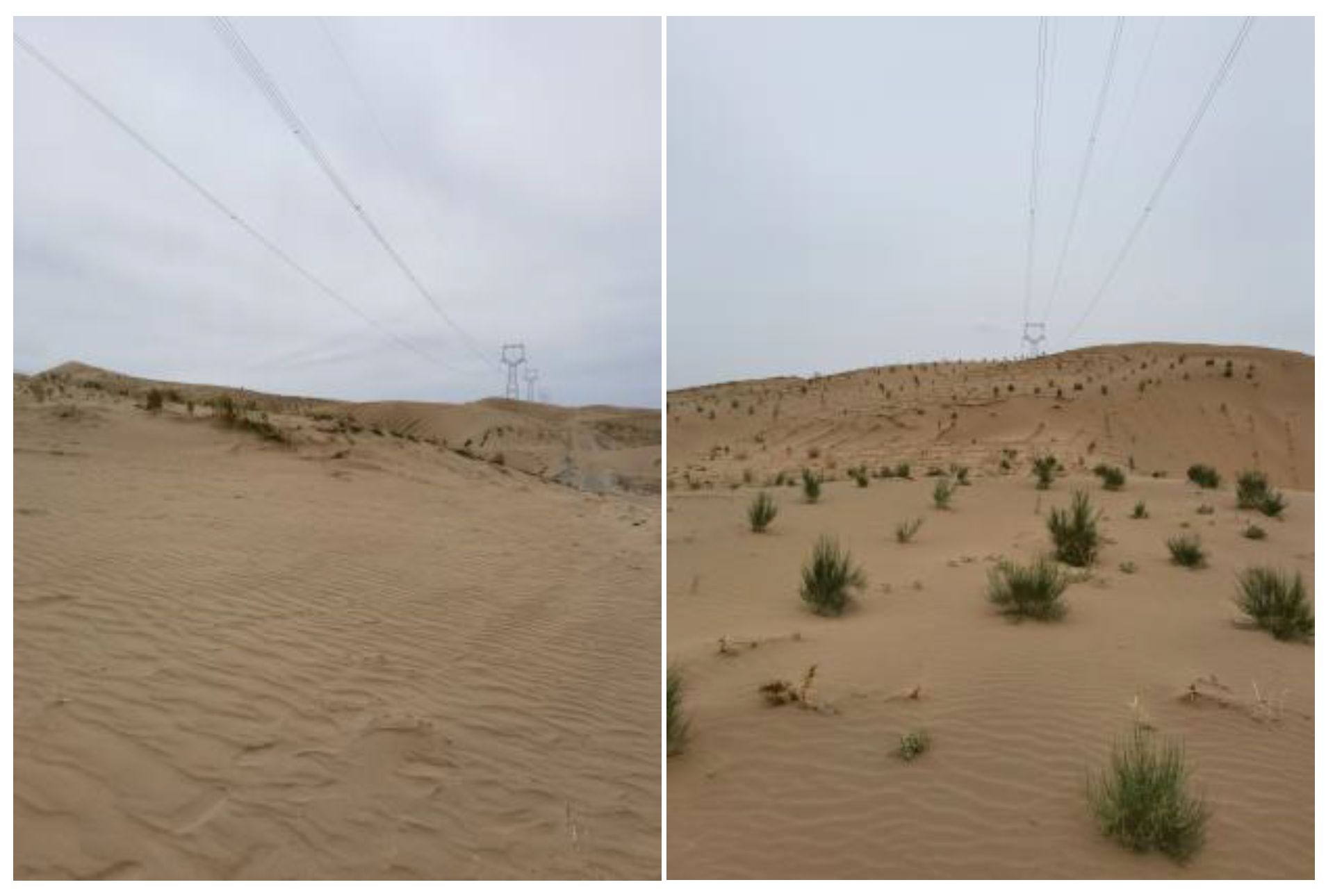
Figure 2.
Test specimen and TSZ-3 strain-controlled triaxial apparatus. (a) Specimen Preparation; (b) TSZ-3 Strain-Controlled Triaxial System.
Figure 2.
Test specimen and TSZ-3 strain-controlled triaxial apparatus. (a) Specimen Preparation; (b) TSZ-3 Strain-Controlled Triaxial System.
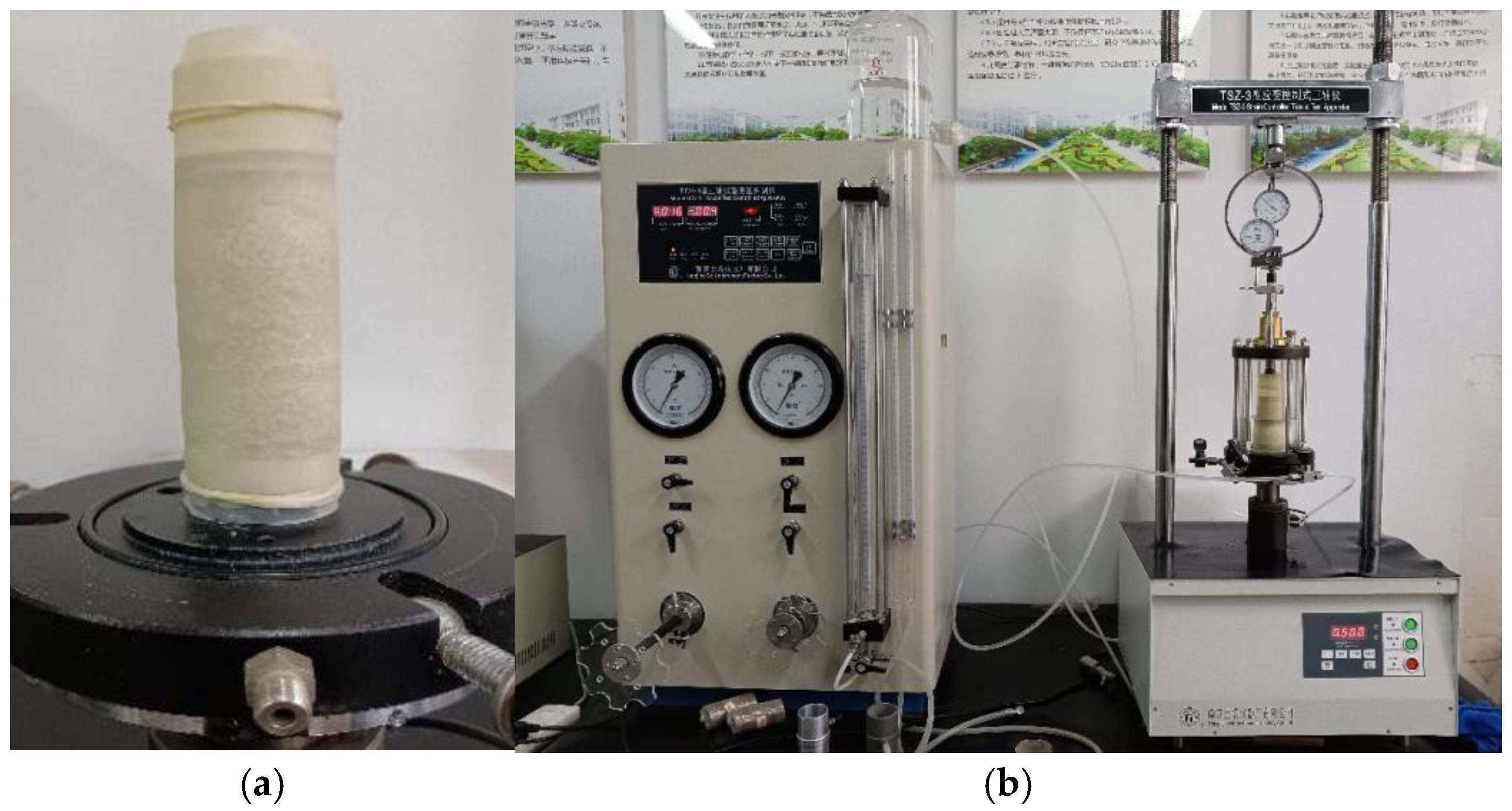
Figure 3.
Test scheme of helical anchor. (a) Axial Compressive Load Test; (b) Axial Tensile Load Test (Uplift Test).
Figure 3.
Test scheme of helical anchor. (a) Axial Compressive Load Test; (b) Axial Tensile Load Test (Uplift Test).

Figure 4.
Load-displacement curves.
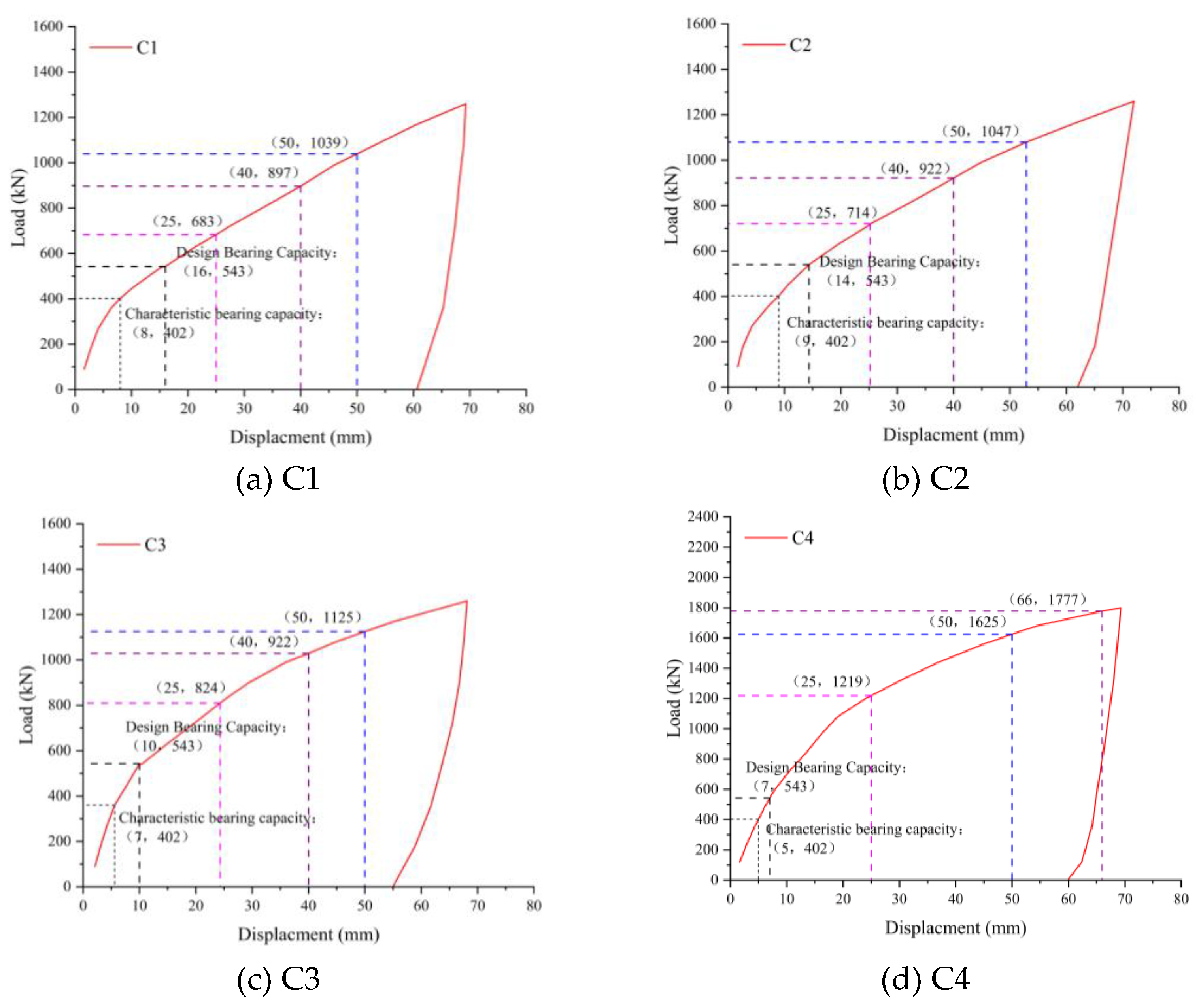
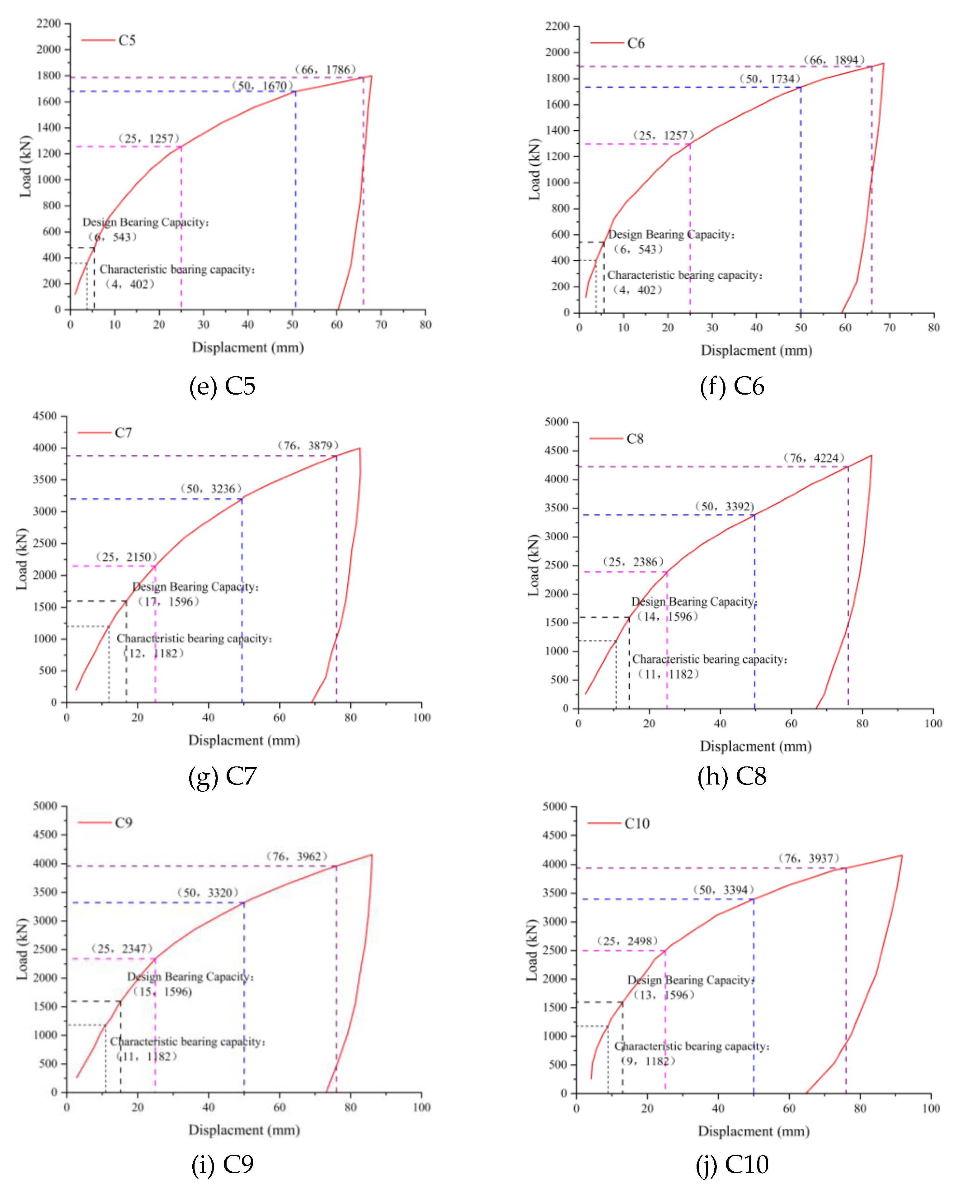
Figure 5.
Load distribution patterns of CS and IB models. (a) CS model; (b) IB model.
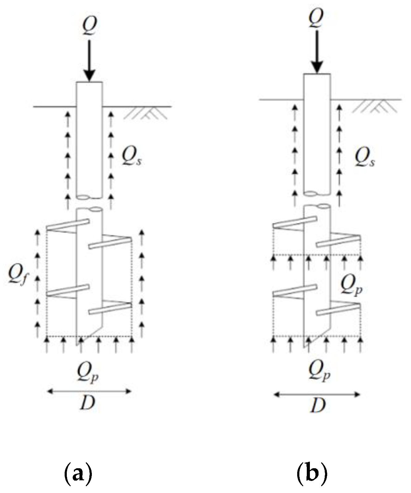
Figure 6.
Reference coefficients in design codes. (a) Lateral earth pressure coefficient; (b) Uplift bearing capacity coefficient.
Figure 6.
Reference coefficients in design codes. (a) Lateral earth pressure coefficient; (b) Uplift bearing capacity coefficient.
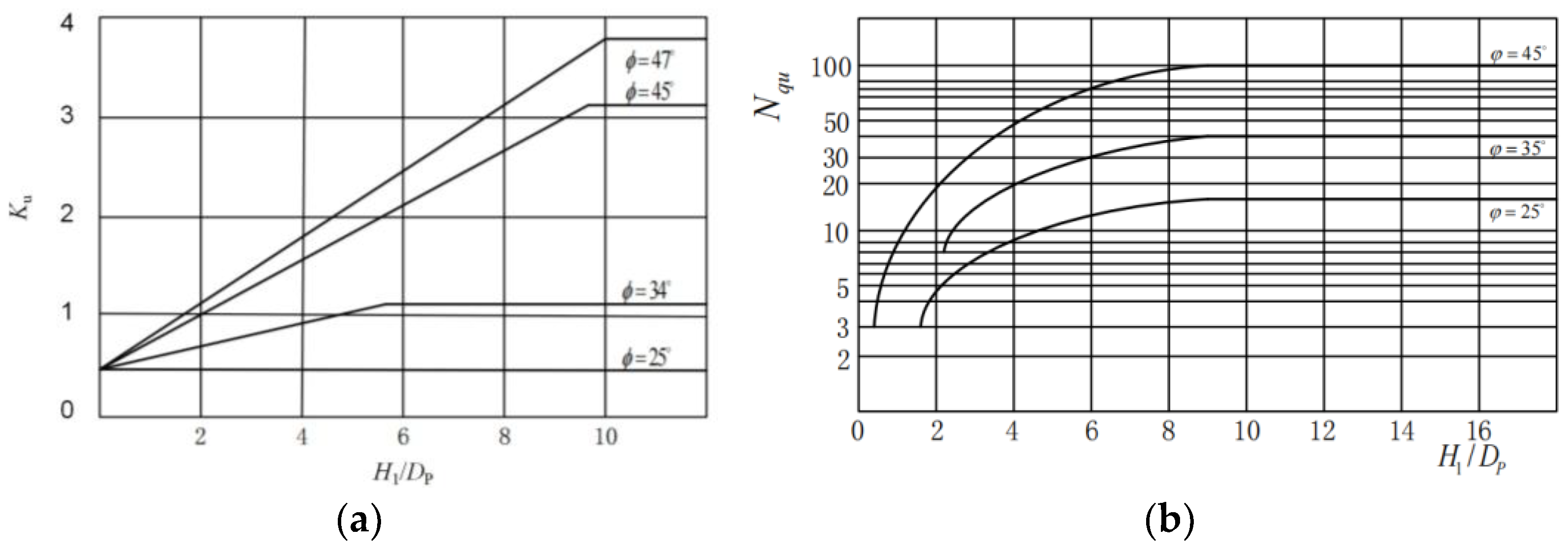
Figure 7.
Numerical model.
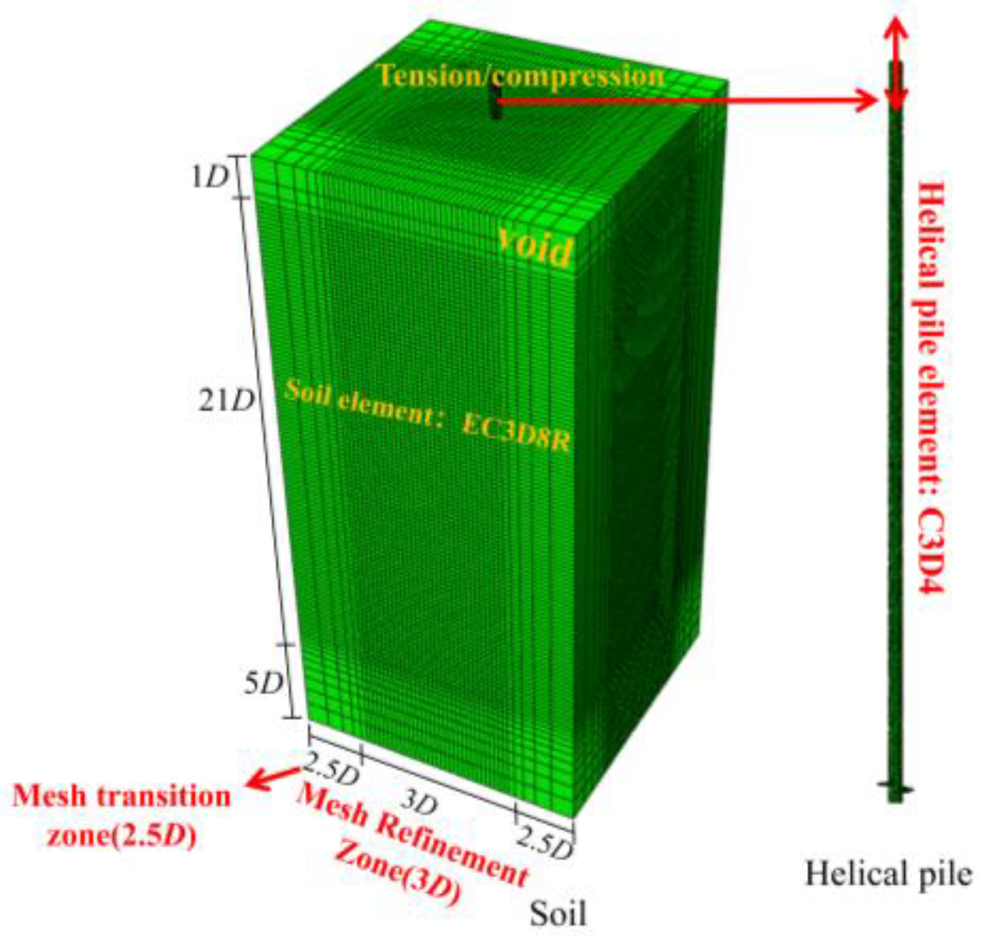
Figure 8.
Load-displacement comparison curves between numerical simulations and field tests.
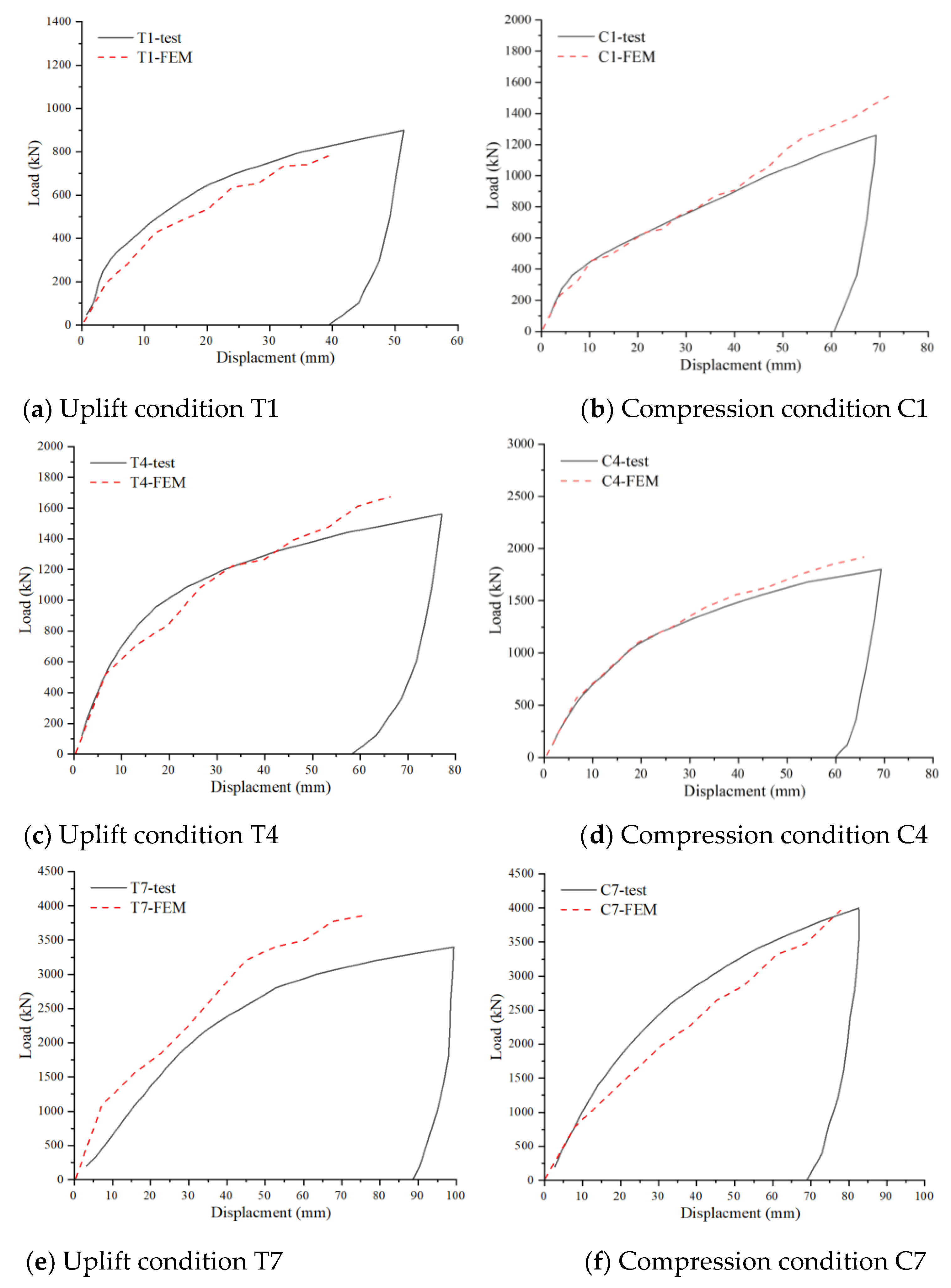
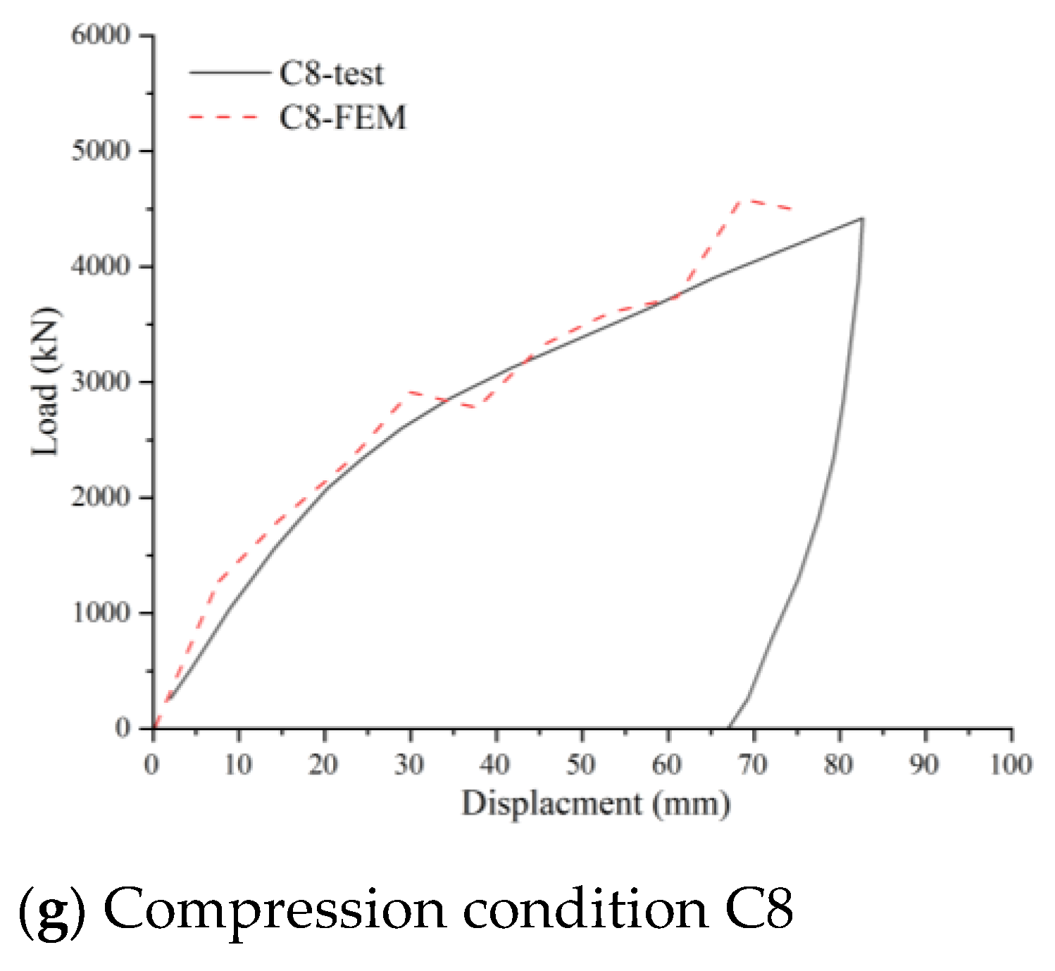
Figure 9.
PEEQ (equivalent plastic strain) contours at ultimate bearing capacity.

Figure 10.
von Mises stress contours for Case C4.
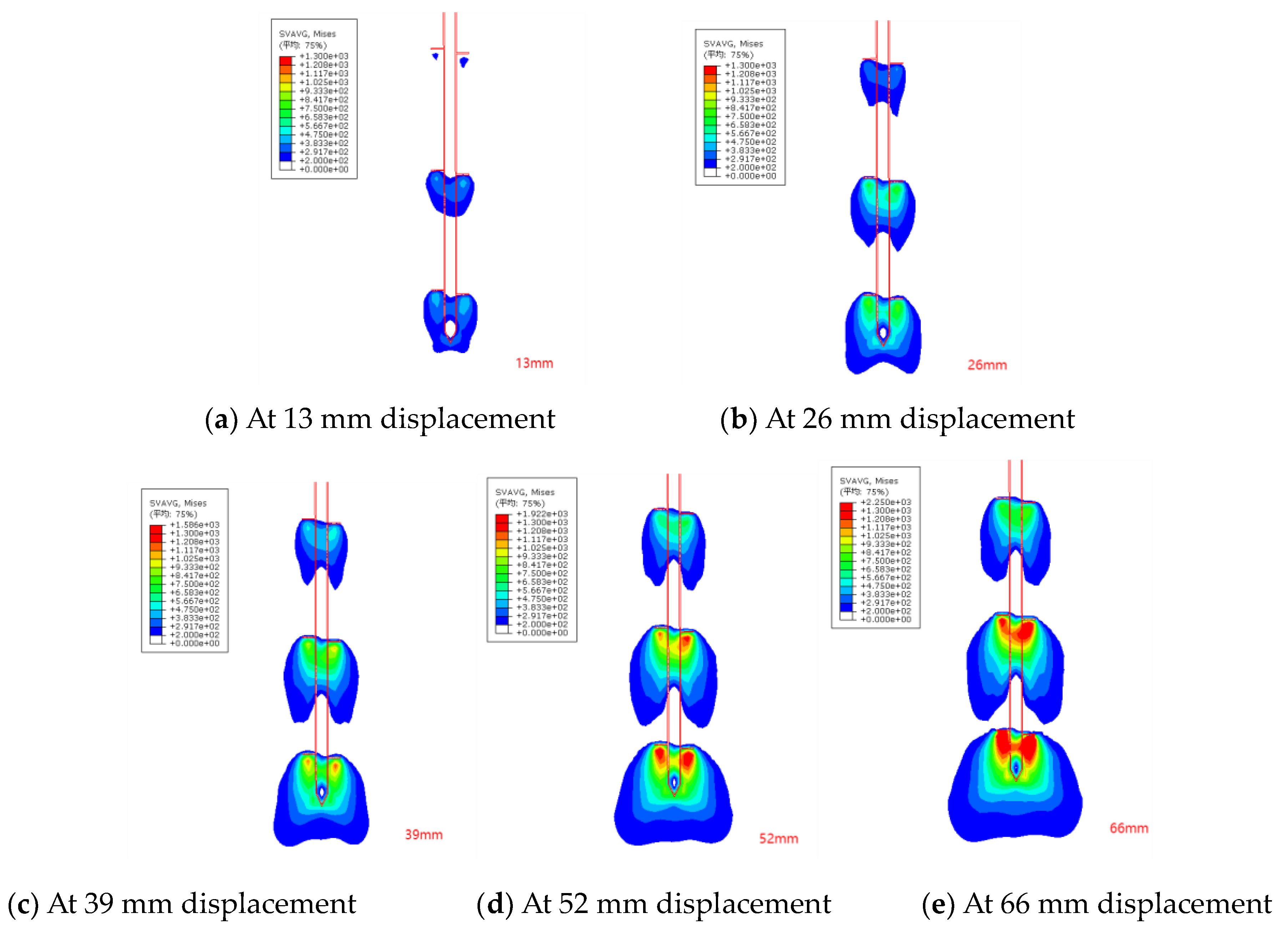
Figure 11.
PEEQ (equivalent plastic strain) contours for Case C4.
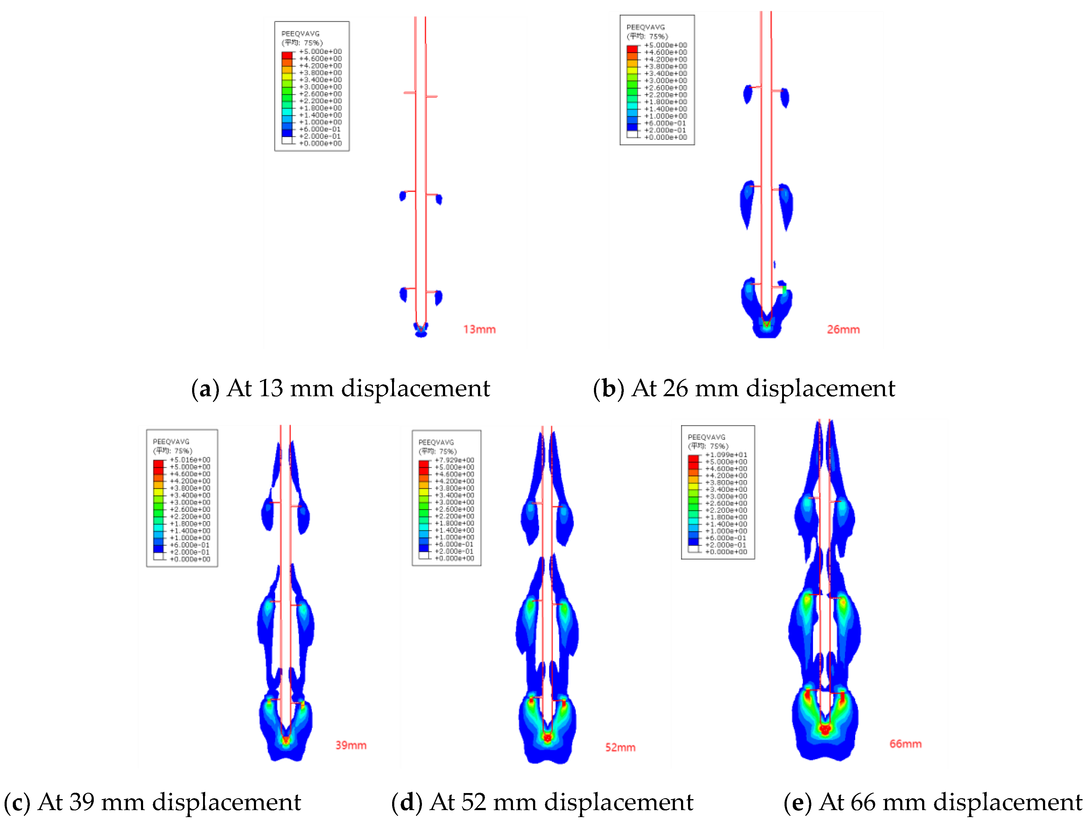
Figure 12.
Comparison of bearing capacity under uplift versus compressive loading conditions.
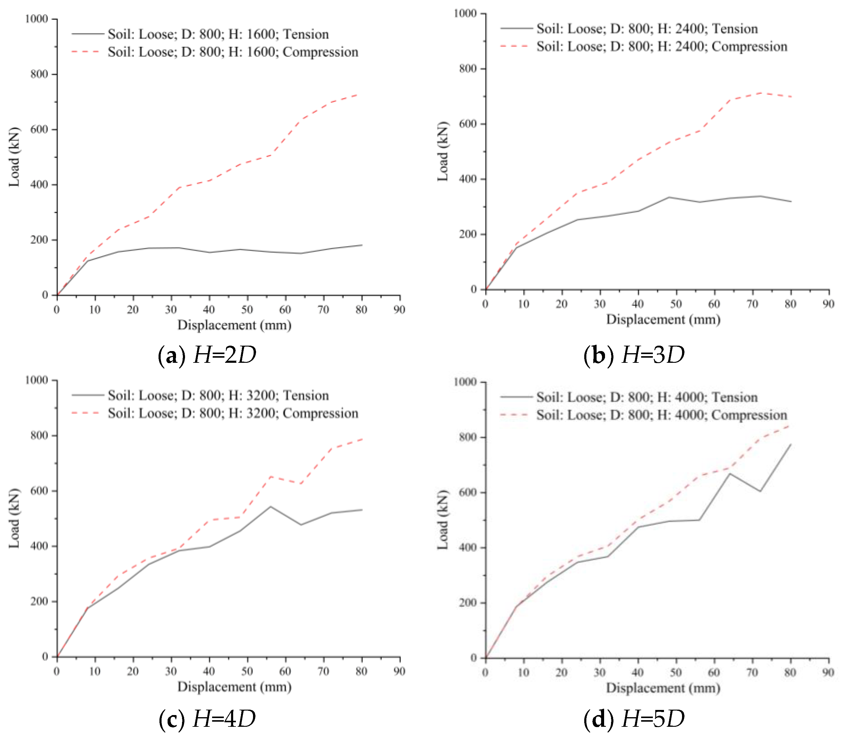
Figure 13.
Plastic strain contours under uplift and compressive loading (anchor rod and soil boundaries outlined in red).
Figure 13.
Plastic strain contours under uplift and compressive loading (anchor rod and soil boundaries outlined in red).
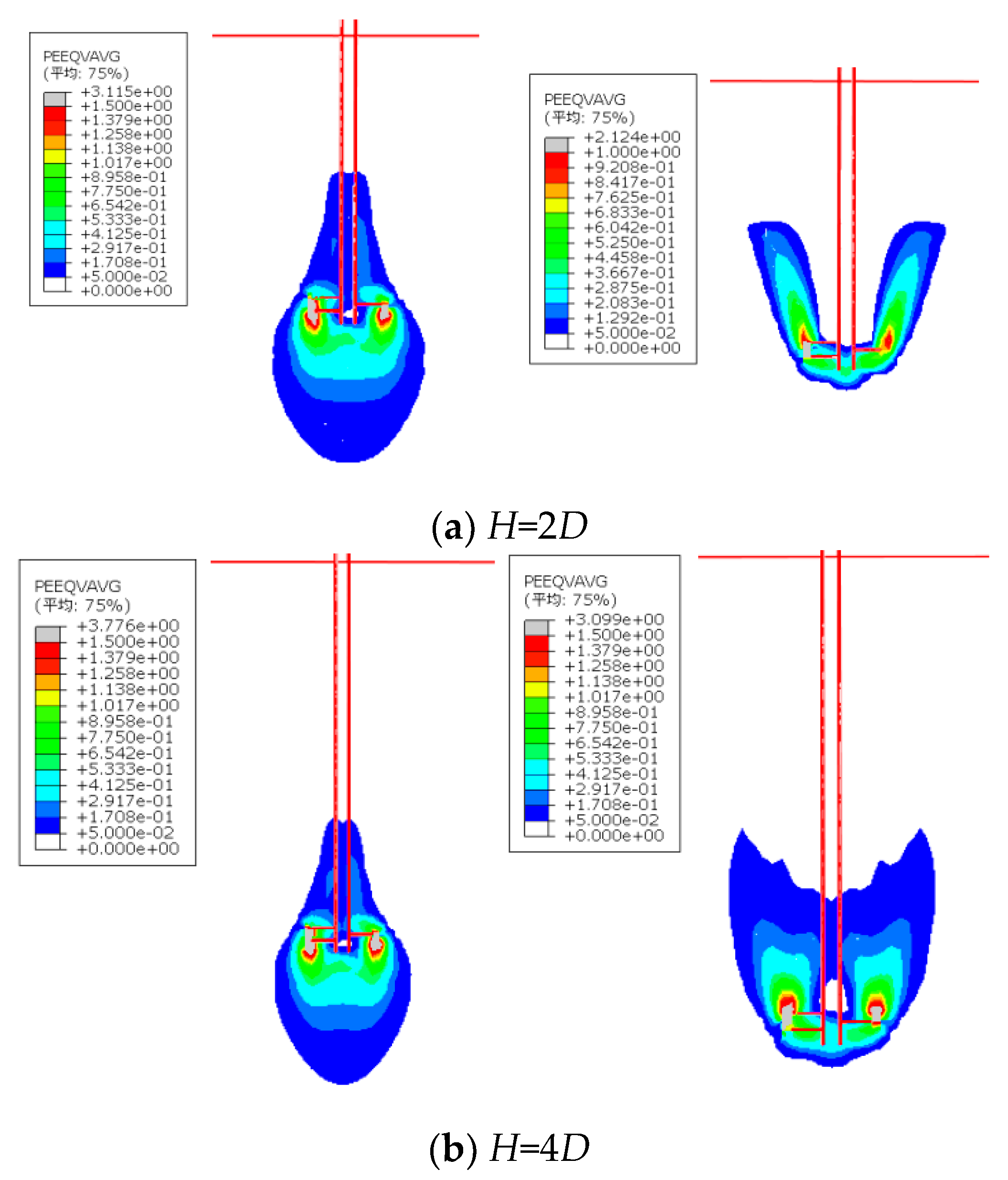
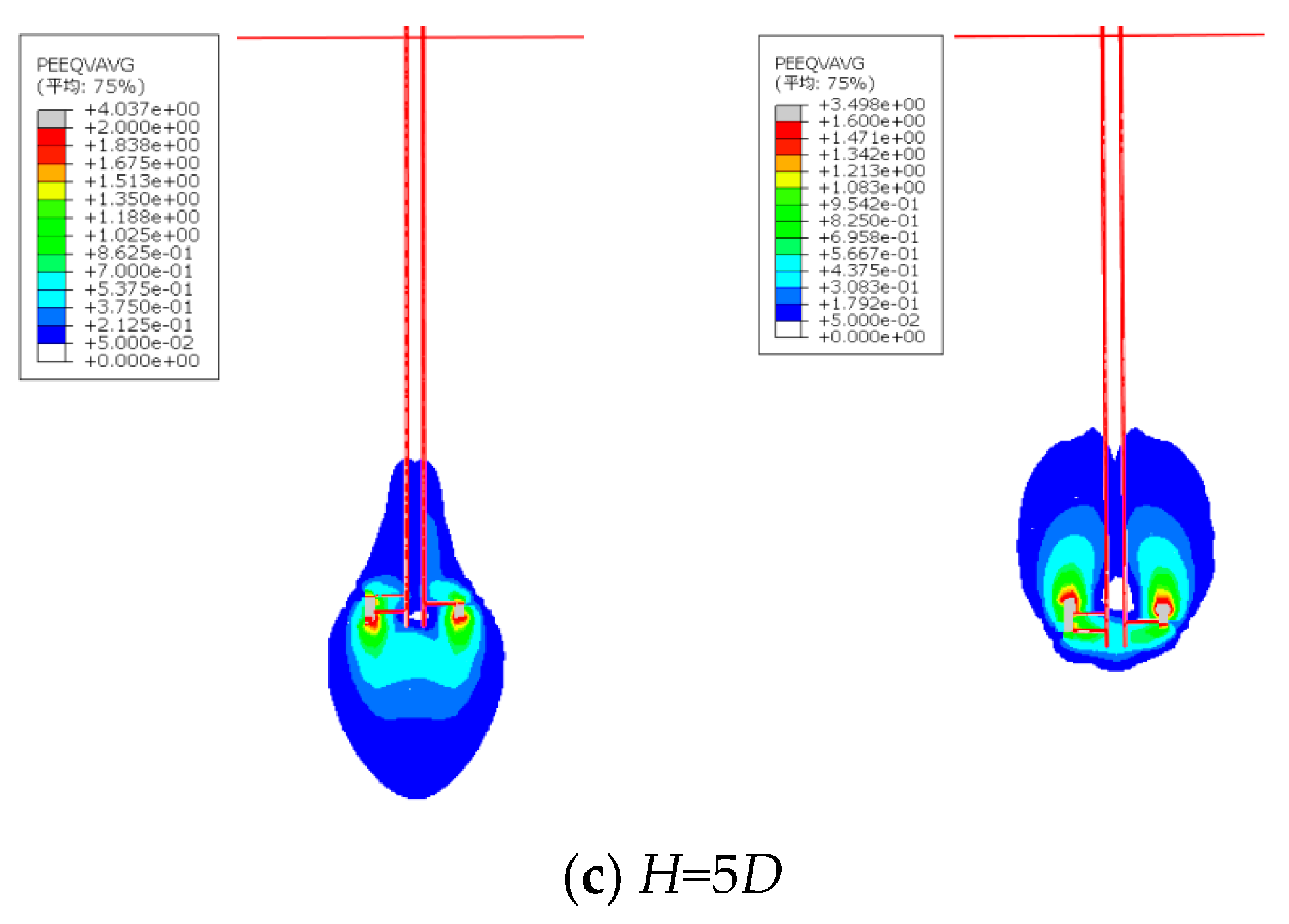
Figure 14.
Numerical plastic strain contours for double-helix anchors with 800-mm plate diameters.
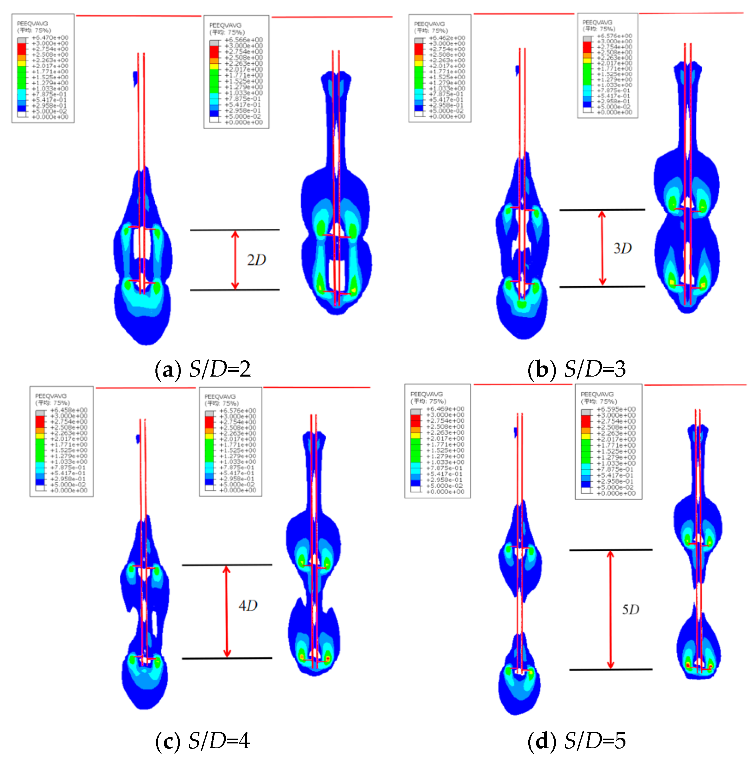
Figure 15.
Schematic diagram of K-fold cross-validation.
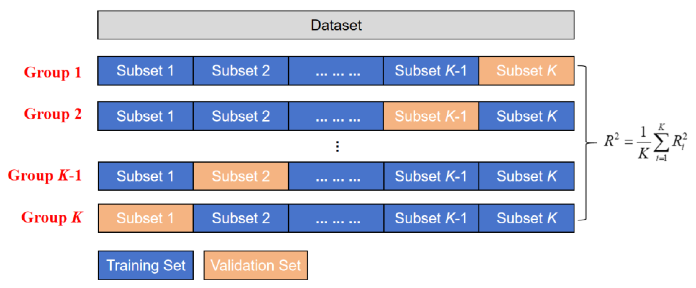
Figure 16.
Comparison of machine learning prediction accuracy.
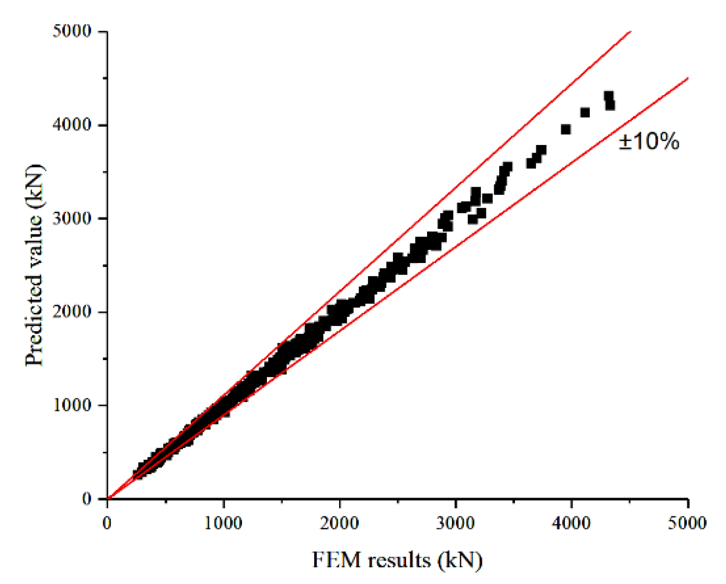
Figure 17.
Feature importance in the machine learning-based compressive capacity prediction model. (a) Feature Importance (Gain); (b) Feature Importance (Weight); (c) Feature Importance (Cover).
Figure 17.
Feature importance in the machine learning-based compressive capacity prediction model. (a) Feature Importance (Gain); (b) Feature Importance (Weight); (c) Feature Importance (Cover).
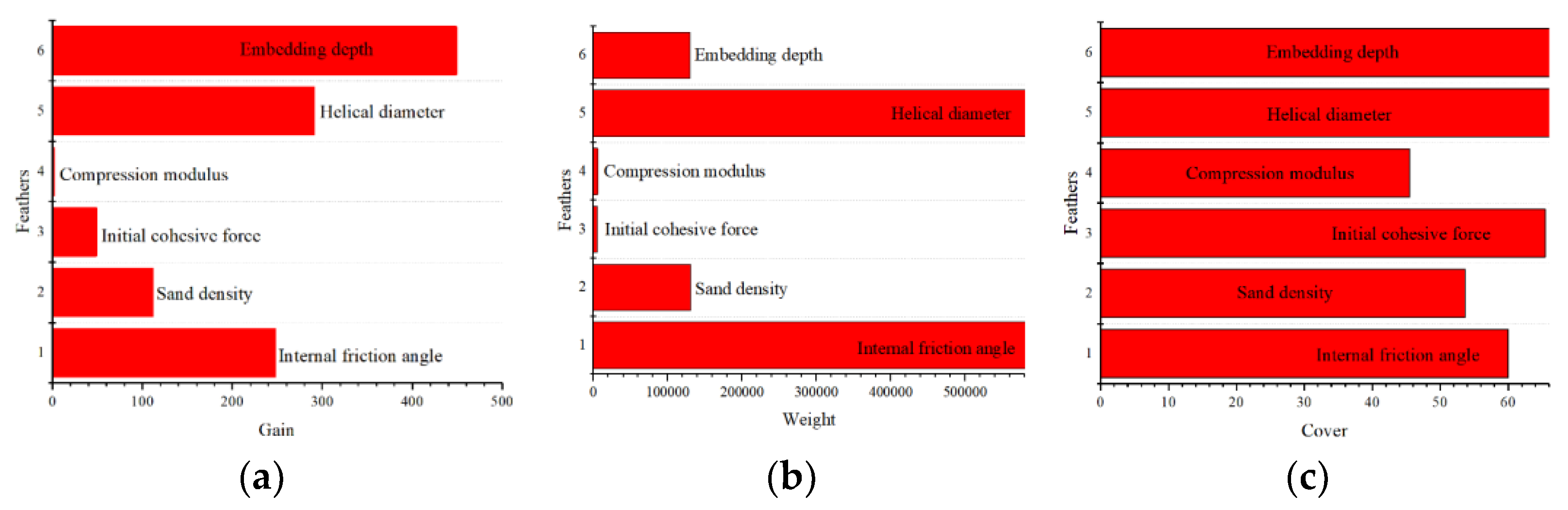
Figure 18.
Compressive capacity factor (Nqu) versus embedment ratio (H/D).
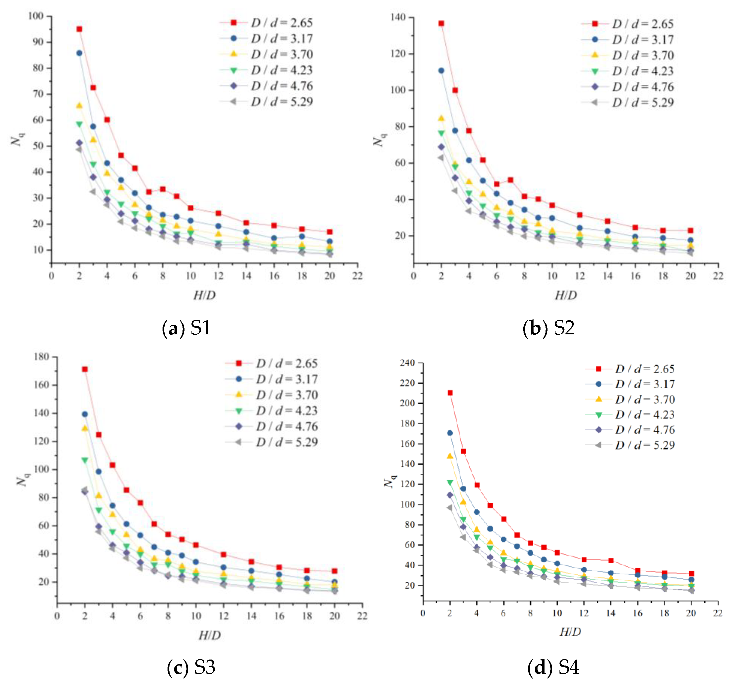
Figure 19.
Derivation workflow for the compressive capacity factor (Nqu) formulation.
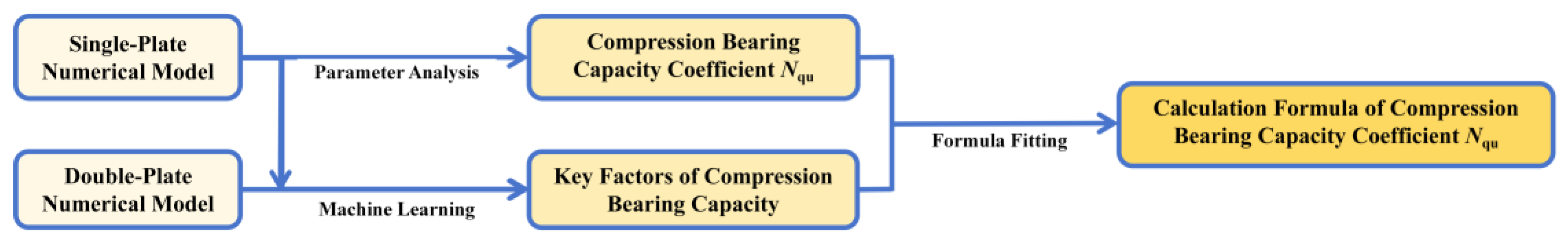
Figure 20.
Fitting curves for lateral earth pressure coefficients in aeolian sands.
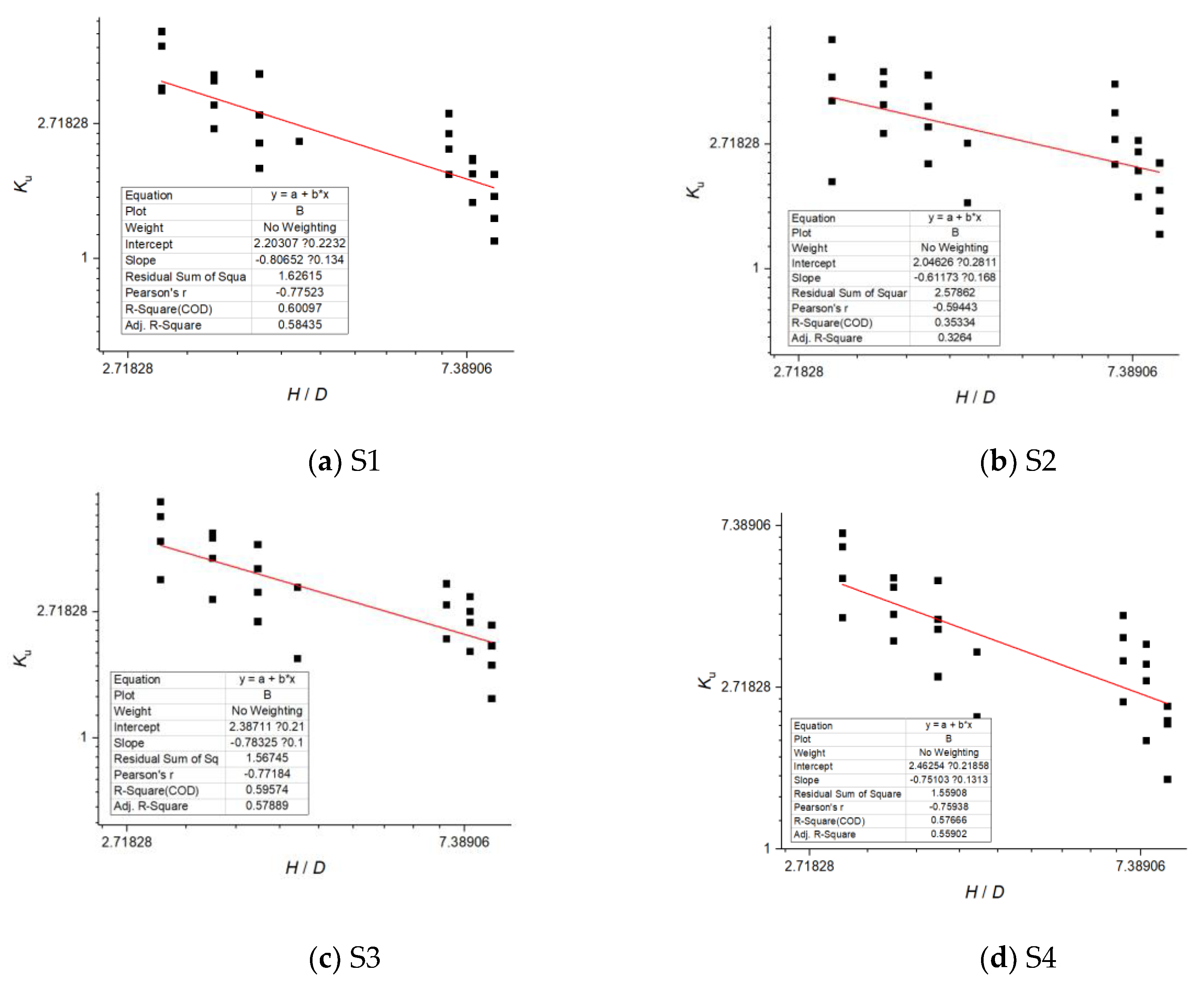
Figure 21.
Derivation workflow for the lateral earth pressure coefficient formulation.
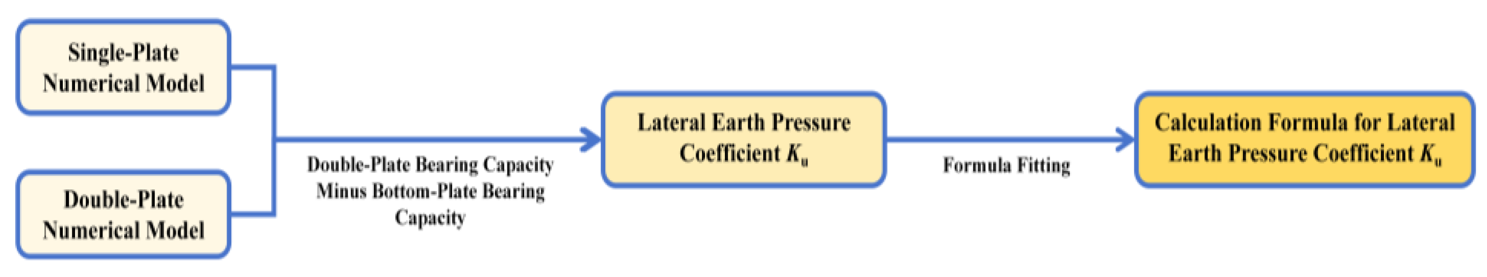
Table 1.
Geological parameters of test site.
| No. | Dense state of sandy soil |
Ρ (g/cm3) |
σ3 (kPa) |
Φ (°) |
Es (MPa) |
H (m) |
|---|---|---|---|---|---|---|
| S1 | Loose sand | 1.60 | 100 | 36 | 20 | 3 |
| 200 | ||||||
| 300 | ||||||
| S2 | Medium loose sand | 1.70 | 100 | 37 | 30 | 0.75 |
| 200 | ||||||
| 300 | ||||||
| S3 | Medium dense sand | 1.80 | 100 | 39 | 40 | 3.5 |
| 200 | ||||||
| 300 | ||||||
| S4 | Dense sand | 1.90 | 100 | 42 | 50 | 8 |
| 200 | ||||||
| 300 |
Note: ρ - natural density; σ3 - confining pressure; φ - internal friction angle; Es - constrained modulus; h - soil layer thickness.
Table 2.
Parameters of helical anchor test specimens.
| No. | Number of Helices | Helix diameter (mm) | Shaft outer diameter (mm) | Helix spacing (mm) | Embedment depth of bottom helix (m) | Embedment depth of top helix (m) | Installation inclination |
|---|---|---|---|---|---|---|---|
| C1 | 3 | 400 | 219 | 1800 | 7.2 | 3.6 | 8.1° inclination |
| C2 | 3 | 400 | 219 | 1800 | 7.2 | 3.6 | |
| C3 | 3 | 400 | 219 | 1800 | 7.2 | 3.6 | |
| C4 | 3 | 660 | 219 | 1976 | 7.26 | 3.3 | Vertical anchor |
| C5 | 3 | 660 | 219 | 1976 | 7.26 | 3.3 | |
| C6 | 3 | 660 | 219 | 1976 | 7.26 | 3.3 | |
| C7 | 3 | 760 | 245 | 2280 | 8.42 | 3.8 | |
| C8 | 4 | 760 | 245 | 2280 | 10.7 | 3.8 | |
| C9 | 4 | 760 | 245 | 2280 | 10.7 | 3.8 | |
| C10 | 4 | 760 | 245 | 2280 | 10.7 | 3.8 |
Table 3.
Field test performance data.
| Specimen ID | Ultimate Load at 0.1D (kN) | Capacity at 50mm Disp. (kN) | Capacity at 25mm Disp. (kN) | Code-Calculated Ultimate (kN) | Code/Test Ratio |
|---|---|---|---|---|---|
| C1 | 897 | 1039 | 683 | 502.947 | 0.56 |
| C2 | 922 | 1047 | 714 | 502.947 | 0.54 |
| C3 | 1029 | 1125 | 824 | 502.947 | 0.48 |
| C4 | 1777 | 1625 | 1219 | 1501.46 | 0.84 |
| C5 | 1786 | 1670 | 1257 | 1501.46 | 0.84 |
| C6 | 1894 | 1734 | 1297 | 1501.46 | 0.79 |
| C7 | 3879 | 3236 | 2150 | 2406.02 | 0.62 |
| C8 | 4224 | 3392 | 2386 | 3299.74 | 0.78 |
| C9 | 3962 | 3320 | 2347 | 3299.74 | 0.83 |
| C10 | 3937 | 3394 | 2498 | 3299.74 | 0.84 |
| Mean value | 0.712 | ||||
| Variance | 0.019 | ||||
Table 4.
Parameters of helical anchor.
| Type | Density ρ/(g/cm3) |
Elastic modulus E/kPa |
Poisson’s ratio |
|---|---|---|---|
| Helical anchor | 7.85 | 2.06×10⁸ | 0.3 |
Table 5.
Parameters of soil layer.
| Soil layer | Thickness of soil (m) | Density ρ/(g/cm3) |
Elastic modulus E/kPa |
Poisson’s ratio | Internal friction angle φ (°) | Dilatancy angle (°) |
| Soil-1 | 3 | 1.6 | 20000 | 0.2 | 36 | 18 |
| Soil-2 | 0.75 | 1.7 | 30000 | 0.2 | 37 | 18.5 |
| Soil-3 | 3.5 | 1.8 | 40000 | 0.2 | 39 | 19.5 |
| Soil-4 | 8 | 1.9 | 50000 | 0.2 | 42 | 21 |
Table 6.
Numerical modeling parameters for single-plate helical anchors.
| D (mm) | Embedment depth (mm) | |||||||||||||
|---|---|---|---|---|---|---|---|---|---|---|---|---|---|---|
| 500 | 1000 | 1500 | 2000 | 2500 | 3000 | 3500 | 4000 | 4500 | 5000 | 6000 | 7000 | 8000 | 9000 | 10000 |
| 600 | 1200 | 1800 | 2400 | 3000 | 3600 | 4200 | 4800 | 5400 | 6000 | 7200 | 8400 | 9600 | 10800 | 12000 |
| 700 | 1400 | 2100 | 2800 | 3500 | 4200 | 4900 | 5600 | 6300 | 7000 | 8400 | 9800 | 11200 | 12600 | 14000 |
| 800 | 1600 | 2400 | 3200 | 4000 | 4800 | 5600 | 6400 | 7200 | 8000 | 9600 | 11200 | 12800 | 14400 | 16000 |
| 900 | 1800 | 2700 | 3600 | 4500 | 5400 | 6300 | 7200 | 8100 | 9000 | 10800 | 12600 | 14400 | 16200 | 18000 |
| 1000 | 2000 | 3000 | 4000 | 5000 | 6000 | 7000 | 8000 | 9000 | 10000 | 12000 | 14000 | 16000 | 18000 | 20000 |
Table 7.
Numerical modeling parameters for twin-plate helical anchors.
| D (mm) | Top Plate Embedment Depth (mm) | Helix plate spacing (mm) | ||||
|---|---|---|---|---|---|---|
| 500 | 1000 | 1000 | 1500 | 2000 | 2500 | 3000 |
| 3000 | 1000 | 1500 | 2000 | 2500 | 3000 | |
| 800 | 1600 | 1600 | 2400 | 3200 | 4000 | 4800 |
| 4800 | 1600 | 2400 | 3200 | 4000 | 4800 | |
Table 8.
Hyperparameter values of the optimal model.
| Model hyperparameters | Values for uplift training | Values for compressive training |
|---|---|---|
| Max Depths | 5 | 4 |
| etas | 0.1489 | 0.1435 |
| subsamples | 0.6272 | 0.6581 |
| Colsample Bytrees | 0.7806 | 0.6983 |
| gammas | 0.0045 | 0.0001 |
| min child weights | 3 | 2 |
| lambdas | 0.7133 | 0.6706 |
| alphas | 0.6977 | 0.6994 |
Disclaimer/Publisher’s Note: The statements, opinions and data contained in all publications are solely those of the individual author(s) and contributor(s) and not of MDPI and/or the editor(s). MDPI and/or the editor(s) disclaim responsibility for any injury to people or property resulting from any ideas, methods, instructions or products referred to in the content. |
© 2025 by the authors. Licensee MDPI, Basel, Switzerland. This article is an open access article distributed under the terms and conditions of the Creative Commons Attribution (CC BY) license (http://creativecommons.org/licenses/by/4.0/).
Copyright: This open access article is published under a Creative Commons CC BY 4.0 license, which permit the free download, distribution, and reuse, provided that the author and preprint are cited in any reuse.


