
Submitted:
20 June 2025
Posted:
20 June 2025
You are already at the latest version
Abstract
Length of stay (LoS) is a critical metric in healthcare management, influenced by various factors, includingthe matching between patients and physicians. This encompasses elements such as the quality of the patient–physician relationship, personality compatibility, and the alignment between the patient’s disease domainand the physician’s clinical expertise—all of which significantly affect LoS. Appropriately matching patientswith physicians can improve the hospitalization experience and reduce LoS; however, most predictivemodels rely primarily on patient-specific information. To address this gap, we employed a deep learning(DL) model—Cyclic Dual Latent Discovery (CDLD)—to predict LoS by incorporating patient–physicianmatching. The model was evaluated using the Medical Information Mart for Intensive Care (MIMIC-IV)version 3.1. CDLD discovers latent trait representations for each patient and physician from their interactiondata, which are then used to predict LoS. The model predicts both overall LoS and duration-specificsubgroups, including short (<5 days) and long (>5 days) stays. Performance evaluation using root meansquare error (RMSE) with 10-fold cross-validation yielded RMSEs of 0.0212 for the full dataset, 0.1767 forthe short-stay group, and 0.1561 for the long-stay group. As this is the first study to incorporate patient–physician matching into LoS prediction, no direct baselines exist. To validate the significance of thediscovered latent traits, we conducted indirect comparisons using common machine learning models—simple deep neural network, XGBoost, CatBoost, and LightGBM—with and without the inclusion of theselatent traits. Across all models, incorporating latent traits consistently improved performance, with anaverage RMSE reduction of 4.6280%. Despite limited prior research on incorporating patient–physicianmatching into LoS prediction, our findings underscore its significant impact and highlight its potential foroptimizing patient assignments and promoting personalized healthcare.
Keywords:
length of stay
; patient-physician matching
; deep learning
; health personnel
; cyclic dual latentdiscovery
1. Introduction
Length of stay (LoS) is defined as the duration of a patient’s hospitalization, from admission to discharge. It serves as a key metric reflecting the consumption of medical resources and the performance of hospital systems, including factors such as diagnostic accuracy and the effectiveness of therapeutic strategies. Accurate LoS prediction is crucial for optimizing hospital resource allocation and reducing healthcare costs. By anticipating LoS, hospital administrators can allocate resources more efficiently, improve patient flow, enhance patient safety, and boost overall operational effectiveness. Accordingly, developing reliable LoS prediction models is critical for improving patient care and hospital performance [1,2,3]. LoS is known to be influenced by numerous factors, including patient demographics, physician characteristics, treatment complexity, the doctor–patient relationship, and discharge planning [4].
One significant factor influencing LoS is patient–physician matching. When patient–physician matching is optimal, patients tend to experience better treatment outcomes, foster trust, higher satisfaction, and improved adherence to medical recommendations [5,6,7]. For physicians, a good match with the patient facilitates more effective communication, enables a better understanding of patient needs, and supports more efficient care delivery—ultimately enhancing care coordination and improving patient outcomes [8,9]. Patient-physician matching encompasses various elements such as physician interventions and skills, professional ethics, training background, physician and patient personality, disease domain, and the quality of the doctor–patient relationship. All of these aspects can significantly impact patient care [10,11]. Several studies have demonstrated the clinical importance of such matching: racial concordance between patients and physicians has been associated with lower mortality rates [12], while gender concordance has also shown measurable effects on patient survival [13]. Furthermore, alignment in cultural understanding and communication styles has been linked to improved treatment adherence and better survival outcomes [14]. These findings underscore that effective patient–physician matching can have life-saving implications. Accordingly, fostering well-aligned patient–physician relationships advances healthcare delivery and policy, and can translate into improved outcomes such as reduced LoS [15,16,17]. To effectively reflect patient–physician matching in LoS prediction, it is essential to incorporate not only patient information but also physician characteristics. However, previous LoS prediction models have largely overlooked the role of the physician [3,4,18]. This gap in prior work highlights the novelty of our approach, which explicitly incorporates the physician’s influence on LoS. By comparing predicted LoS under different matching configurations, our current approach has the potential to reveal physician latent factors that contribute to effective patient–physician alignment and better healthcare outcomes.
To address this gap, we applied the Cyclic Dual Latent Discovery (CDLD) model [19], leveraging patient–physician matching as a predictive factor for LoS. CDLD jointly learns latent representations for both entities. These latent traits are then incorporated into separate LoS prediction models. We applied CDLD to the large dataset, Medical Information Mart for Intensive Care (MIMIC-IV) version 3.1 after preprocessing [20]. Because, to our knowledge, this is the first study to incorporate patient–physician matching into LoS prediction, there is no established baseline for direct comparison. Therefore, we performed indirect comparisons using alternative machine learning models to evaluate the effectiveness of our discovered latent traits by our approach.
In summary, we introduce a novel deep learning (DL) approach for LoS prediction that incorporates patient–physician matching. The following sections detail our data preprocessing and entity construction steps, describe the CDLD model architecture and training procedure, present the prediction results (including indirect validation experiments), and discuss the implications and limitations of our findings.
2. Related Work
A wide range of approaches have been explored for LoS prediction, spanning from traditional statistical models to modern machine learning and DL techniques [3,4]. Early studies often relied on linear regression or survival analysis to estimate LoS and patient flow [2,4]. More recently, data-driven models have become dominant: many studies apply machine learning algorithms (e.g., random forests, gradient boosting machines) or neural networks to predict LoS, as noted in contemporary reviews [3,4]. These models generally leverage patient-centric features such as age, sex, diagnoses, comorbidity indices, vital signs, and laboratory results, and are sometimes supplemented with hospital administrative details (e.g., admission source or service unit).
Recent studies have also begun incorporating multi-modal electronic health record (EHR) data to improve LoS prediction accuracy. For example, Chen et al. developed a DL model that combined structured EHR variables with unstructured clinical notes, outperforming models that used only a single data source [21]. Although recent models incorporate multi-modal patient data, no prior LoS prediction model explicitly accounts for the relational dynamics based on patients and physicians matching or physician-specific factors. This omission is particularly significant given the well-established impact of the patient–physician matching and individual physician characteristics on clinical outcomes.
In this study, we apply the CDLD framework to LoS prediction with hyperparameter modifications; the core architecture and training strategy remain the same as in the original CDLD. The CDLD model can discover latent trait representations for both patients and physicians based on their interactions, enabling it to capture the otherwise intangible impact of patient–physician matching on LoS.
3. Method
3.1. Data Preprocessing
We loaded the MIMIC-IV dataset into a structured query environment [22] and calculated LoS by subtracting the “admittime” column from the “dischtime” column from the “admissions.csv”. We then applied a series of filters to remove incomplete or irrelevant records. Specifically, we excluded any admissions with missing key values, negative LoS (which corresponded to organ donor cases), any recorded death time, or an admission type classified as “OBSERVATION” (e.g., “EU OBSERVATION”, “OBSERVATION ADMIT”, “AMBULATORY OBSERVATION”, and “DIRECT OBSERVATION”). We retained only admissions with types indicating standard hospital stays (“DIRECT EMER”, “ELECTIVE”, “EW EMER”, “SURGICAL SAME DAY ADMISSION”, and “URGENT”). Moreover, we treated extremely short stays (LoS ≤ 10 minutes) as outliers and removed them. After applying these criteria, the dataset was reduced from 546,028 admissions to 300,358 (retaining about 55.0% of the original records). The resulting dataset contains only valid, clinically relevant hospitalizations, providing a robust basis for our analysis (Figure 1).
In the filtered dataset, LoS ranged from 13 minutes up to 463,074 minutes (approximately 321 days). It encompassed 149,891 patients and 1,817 physicians across 300,358 hospital admissions. The distribution of LoS was highly skewed toward shorter stays (Figure 2A), which can bias model training by overemphasizing the most common outcomes. To mitigate this, we partitioned the data into short-stay and long-stay groups for separate analysis. Since there is no universal cut-off for defining a “short” hospital stay [23], we selected thresholds informed by prior studies and the characteristics of our data. We defined short LoS as stays lasting more than 2 hours and up to 5 days, aligning with literature on short-stay units [24]; this subset comprised 189,974 admissions (covering 138,044 patients and 1,706 physicians) as shown in Figure 2B. We defined long LoS as > 5 days and ≤ 28 days (Figure 2C), choosing 28 days such that each day in this range had at least 500 records. The long-stay subset contained 104,552 admissions (covering 83,367 patients and 1,506 physicians). For consistency, all LoS values were recorded in minutes in our analysis.
3.2. Entity Representation
The CDLD model is designed to discover latent traits for two types of entities using two coupled latent-trait discoverer networks, and then utilize these discovered traits in the predictor network for the final prediction. In this study, we define the two entities as the patient entity and the physician entity. Each entity representation consists of a set of observed features and a set of latent traits. The features are directly obtained from the MIMIC-IV dataset and preprocessed, whereas the latent traits are initially unknown and randomly initialized, to be discovered by the model during training.
3.2.1. Patient Entity
To construct the feature set for the patient entity, we merged several tables from MIMIC-IV (“admissions.csv”, “patients.csv”, “microbiologyevents.csv”, and “omr.csv”) on the patient identifier (“subject_id”). This integration provided a comprehensive view of each patient’s data. We then performed feature engineering and cleaning as follows:
In “admissions.csv”, we first consolidated rare categories by grouping similar values for categorical attributes (“language” and “race”). We then applied one-hot encoding to categorical variables (“insurance”, “language”, “marital status”, and “race”), converting each category into a binary indicator. Missing entries in these categorical fields were set to “UNKNOWN”. The “gender” was label-encoded (0 = female, 1 = male). We normalized continuous variables “anchor_age” using min–max scaling to range [0,1] for comparability [25-27]. In “microbiologyevents.csv”, “isolate_num” was set to 0 if it had no value. (assuming no isolate grew).
In the "omr.csv", the "eGFR" variable had over 95% missing values and was therefore removed to avoid introducing bias. For the remaining numeric variables, we computed z-scores and excluded entries beyond ±3 standard deviations to minimize the influence of extreme outliers. Special handling was applied to body measurements: if any one of "BMI", "height", or "weight" was missing, it was estimated using the other two via Formula 1 to ensure consistency among these interrelated variables.
After these steps, any remaining missing values were imputed using a random forest model that leveraged correlations among available features to infer plausible values [28]. Additionally, blood pressure data were collected in multiple patient positions (lying, sitting, standing, and orthostatic measurements after 1 and 3 minutes). We averaged the systolic and diastolic readings in each position to create aggregated high blood pressure and low blood pressure features, capturing overall blood pressure trends for each patient. Table 1 provides a summary of all features incorporated into the patient entity, along with their sources and any preprocessing steps.
3.2.2. Physician Entity
To construct the physician entity, we extracted the attending physician identifier from each admission record. In the MIMIC-IV “admissions.csv”, the column “admit_provider_id” indicates the clinician who admitted the patient; we treated each unique provider ID as a distinct physician entity in our model. However, the MIMIC-IV dataset does not contain additional attributes about these physicians (such as specialty, experience, or demographics). Therefore, the physician entity does not have feature variables analogous to the patient features. Instead, each physician is represented only by a unique ID and its associated latent traits (which the CDLD model will discover during training).
3.3. CDLD Model
3.3.1. Cyclic Dual-Network Training Mechanism
Our predictive method is built on the CDLD approach, which is designed to uncover hidden “traits” of two interacting entities. In our context, CDLD uses two parallel neural networks—one dedicated to patients and one to physicians—to discover latent trait for each. CDLD alternates updates between the patient and physician networks in a coordinated loop. During training, it iteratively refines the latent traits by updating one network’s weights while keeping the other network fixed, then swapping roles in the next iteration. In each cycle, one network treats the current latent representation of the other entity as a constant context and learns to better encode its own entity’s traits given that context. For example, when updating the patient network, the physician network’s output is held fixed, and vice versa. This alternating update “locks in” one side of the interaction at a time, allowing the model to progressively capture the interdependent patterns of patient–physician matching without one side overwhelming the learning process. Conceptually, this mirrors an expectation–maximization or alternating optimization procedure, where each network incrementally improves its latent representation of one entity, assuming the other’s latent factors are temporarily accurate. The cyclic dual-network mechanism is crucial for modeling patient–physician matching because it forces the latent traits of each party to co-evolve: the patient representation is learned in the context of how physicians behave, and the physician representation is learned in the context of patient characteristics. Over successive cycles, this yields a pair of latent vectors (one for the patient, one for the physician) that jointly encode their compatibility, which is highly informative for predicting outcomes like LoS based on patient-physician matching.
3.3.2. Two-Stage Model Architecture
We adjusted the network architecture (e.g., the sizes of dense layers) to suit our dataset, ensuring that each network has sufficient capacity to model its entity’s characteristics without overfitting. Batch normalization is applied after each layer to stabilize training by normalizing layer inputs [29, 30], and dropout regularization is used to prevent overfitting [31]. Based on preliminary trials, we set a batch size of 512, which provided a good balance between training speed. with the dropout rate tuned through experimentation. (The overall structure of the patient and physician latent discoverer networks is illustrated in Figure 3)
After training the dual latent trait discoverers, we obtain a discovered latent vector for each patient and each physician. These latent traits are then fed into the predictor network that produces the final LoS prediction. The predictor is a standard feed-forward neural network that receives as input the concatenation of patient and physician latent vectors with patient features. Architecturally, the predictor network is similar in depth and layer structure to an individual latent trait discoverer network, but it does not use cyclic training; instead, it is trained in the usual forward manner on the prediction task. The predictor essentially learns how the interaction of the discovered patient and physician traits translates into LoS. This two-stage design (discoverer followed by predictor) allows the model to first capture who the patient and physician are (in terms of latent factors derived from their interactions) and then use that information to predict what they will achieve together (LoS). We found this separation beneficial for modeling the patient-physician matching: the CDLD discoverer isolates the latent compatibility effects, and the predictor leverages these effects for more accurate LoS prediction.
3.3.3. Model Training Detail
We initially partitioned the data into 90% for training and 10% for hold-out testing. For fair comparison across models, we used the same 80%/10%/10% train/validation/test split and applied 10-fold cross-validation on the training portion to obtain robust performance estimates [32]. Prior to model training, we augmented the training data by adding small random noise (of maximum magnitude 0.1) to LoS values, effectively expanding the training set five-fold. This data augmentation was intended to improve generalization and make the model more robust to overfitting [33].
We first trained the latent trait discoverer networks for 30 epochs, where each epoch was composed of 10 updates alternating between the patient and physician latent trait networks as described above. After the discoverer stage converged, we trained the predictor network for up to 1,000 epochs, using an early stopping criterion to prevent overfitting [34]. We adopted the Mean Squared Error (MSE) [35] as the loss function for both the discovery phase and the prediction phase.
3.4. Comparison Models
In the absence of an established benchmark specific to patient–physician matching, we performed an indirect evaluation of our approach by comparing multiple baseline models with and without the inclusion of latent traits. Specifically, we considered four widely used prediction models as benchmarks: a simple deep neural network (DNN) [36], XGBoost [37], LightGBM [38], and CatBoost [39]. Each model was trained in two configurations: one using only the engineered patient features, and one using the combination of those features plus the discovered patient and physician 32-dimensional latent traits. We represented patient latent traits as “latent_0” through “latent_31”, and physician latent traits as “Latent_0” through “Latent_31”. These latent traits, each represented as a 32-dimensional vector, were directly concatenated with the features and fed into the model as input variables. For a fair comparison, we trained all models on the same dataset of 300,358 admissions, using an identical 80%/20% split for training and testing.
For the simple DNN, we used a feed-forward architecture with three hidden layers of 128, 64, and 32 neurons, respectively, followed by a single output node for regression. We applied the Swish activation function at each hidden layer [40] and included a dropout rate of 0.2 to reduce overfitting [31]. For the tree-based gradient boosting models (XGBoost, LightGBM, and CatBoost), we set each model to use 300 trees/estimators with a learning rate of 0.05 and a maximum tree depth of 7. We also applied subsampling of 80% of the training data for each tree and 80% column sampling (feature subsampling) to further prevent overfitting in these models.
3.4. Evaluation Metrics
We employed Root Mean Square Error (RMSE) as the primary metric to quantify prediction error [41]. Additionally, to assess the consistency of model performance across the cross-validation folds, we calculated the coefficient of variation (CV) of the RMSE [42, 43]. The CV provides a normalized measure of variability (defined as the standard deviation of the RMSE across folds divided by the mean RMSE). Lower CV values indicate more stable performance. (Formula 2)
- CV: Coefficient of variation
- σ: Standard deviation
- μ: Mean
To quantify the contribution of the discovered latent traits, we compared the RMSE results of each model with and without latent traits (as reported in the Results section for the baseline models). In addition to error metrics, we performed a SHapley Additive exPlanations (SHAP) [44] analysis to examine how the inclusion of latent traits alters the models’ decision-making. SHAP provides insight into model interpretation by assigning each feature (including our latent trait features) an important value that represents its contribution to a specific prediction [45-47]. By comparing SHAP outputs for models using only original features versus those using features plus latent traits, we could assess how the latent representations influence feature importance and ultimately the LoS predictions.
4. Results
4.1. CDLD Results
4.1.1. Full-LoS Results
For LoS prediction across the full-LoS dataset, the 10-fold cross-validation yielded an average test RMSE of 0.0219 (±0.0007). The per-fold RMSE values ranged from 0.0212 to 0.0233 (0.0212, 0.0214, 0.0221, 0.0216, 0.0233, 0.0227, 0.0214, 0.0212, 0.0223, and 0.0221), with the best-performing fold achieving an RMSE of 0.0212. The variability across folds was low (CV = 3.18%), indicating consistent performance (Figure 4A).
Given the skewed distribution of LoS in the overall dataset, we further evaluated our model on two subsets (short-LoS and long-LoS) to ensure the performance was robust across different hospitalization durations.
4.1.2. Short-LoS (Between 2 Hours and 5 Days) Results
In the short-LoS subset (LoS between 2 hours and 5 days), the model achieved an average RMSE of 0.1801 (±0.0023) across 10 folds. The per-fold RMSE values ranged from 0.1767 to 0.1828 (0.1820, 0.1828, 0.1823, 0.1767, 0.1768, 0.1781, 0.1790, 0.1805, 0.1812, and 0.1814). The best fold obtained an RMSE of 0.1767. Performance variability was very low (CV = 1.25%), reflecting high stability in this range (Figure 4B).
4.1.3. Long-LoS (Between 5 Days and 28 Days) Results
In the long-LoS subset (LoS between 5 to 28 days), the model’s average RMSE was 0.1597 (±0.0035) over 10 folds. The per-fold RMSE values ranged from 0.1561 to 0.1639 (0.1581, 0.1617, 0.1597, 0.1606, 0.1561, 0.1588, 0.1601, 0.1639, 0.1608, and 0.1571). The best RMSE observed was 0.1561. The model maintained consistent accuracy in this range as well (CV = 1.43% across folds; Figure 4C).
Overall, the low CV values in all scenarios (full, short, and long LoS) indicate minimal variance in the model’s predictive performance. The stability observed across these experiments demonstrates the effectiveness of incorporating patient–physician matching into LoS prediction. Table 2 summarizes the RMSE and CV results for the full dataset as well as the short- and long-LoS subsets [48].
4.2. Comparative Results
4.2.1. With or Without Latent Trait Comparison
In comparative experiments, all four benchmark models showed improved accuracy when latent traits were added. The simple DNN’s RMSE improved from 0.0228 (features only) to 0.0214 (features + latent). Similarly, XGBoost’s RMSE dropped from 0.0226 to 0.0217, LightGBM’s from 0.0226 to 0.0216, and CatBoost’s from 0.0227 to 0.0218 after incorporating latent traits. On average, these reductions correspond to roughly a 4.63% decrease in RMSE. This consistent improvement across diverse models suggests that the latent patient–physician matching information enhances predictive performance regardless of the modeling approach (Table 3).
4.2.2. SHAP Analysis: Feature-Only vs Feature+Latent
The SHAP analysis for XGBoost highlighted clear shifts when latent traits were added. For XGBoost using feature-only dataset, the top SHAP features were ‘isolate_num’, ‘lower_count’, ‘upper_count’, ‘high_BP’, and ‘anchor_age’ (Figure 5A, Appendix A1, 2). However, after introducing latent traits, many of those original SHAP features became less influential. Instead, latent dimensions (e.g., ‘Latent_3’, ‘Latent_14’, ‘Latent_15’, etc.) emerged among the most important predictors – in fact, 15 of the top 20 SHAP features in the model were latent traits in the feature+latent dataset (Figure 5B, Appendix A3, 4). This shift suggests that by including latent traits, XGBoost was able to capture hidden patient–physician matching effects that improve its LoS predictive power.
We observed the same pattern in LightGBM and CatBoost. For LightGBM without latent traits, the top SHAP features were similar features (‘isolate_num’, ‘upper_count’, ‘marital_status_MARRIED’, ‘anchor_age’, etc.) (Figure 5C, Appendix A5, 6). Once latent traits were included, 15 of the top 20 SHAP features were latent dimensions, indicating that the latent traits had become the dominant drivers of the model’s predictions (Figure 5D, Appendix A7, 8). CatBoost showed a comparable shift: latent dimensions like ‘Latent_3’, ‘Latent_14’, and ‘Latent_15’ moved into the top ranks (again about 15 of the top 20) (Figure 5F, Appendix A11, 12), displacing many of the original SHAP features that previously ranked highest in the feature-only dataset (Figure 5E, Appendix A9, 10). These consistent trends across XGBoost, LightGBM, and CatBoost confirm that adding latent patient–physician traits significantly changes the SHAP feature importance landscape in favor of the latent traits.
Overall, the SHAP analyses confirm that including latent traits of both patients and physicians fundamentally alters and often improves the models’ decision-making process. In every model examined, latent traits not only contributed to increased accuracy but also assumed top positions in SHAP feature importance rankings, underscoring their value in capturing complex patterns that raw features alone cannot capture. These findings demonstrate that our approach effectively captures the underlying structure of patient–physician matching, which in turn leads to better LoS predictions (Figure 5).
The feature impact plot’s x-axis represents the SHAP value, which shows the direction and magnitude of each feature's effect on the model output. The y-axis lists the top 20 most influential features, ranked based on their SHAP value distributions. For a high-resolution version of this figure, please refer to Appendix A.
5. Discussion and Limitations
5.1. Discussion
Our results demonstrate that reflecting patient-physician matching into LoS predictions provides measurable benefits. The proposed CDLD model, which couples patient and physician entities in a cyclic training process, achieved stable LoS predictions within the extensive MIMIC-IV dataset. This improvement confirms that differences in physician practice styles can significantly influence patient outcomes like LoS. In fact, accounting for the physician’s latent characteristics captured intangible variability that traditional patient-only models miss, underscoring the value of including physician information and patient-physician matching in predictive modeling. These findings support prior observations that physician factors impact hospital metrics [9,12,13,14], and they validate our hypothesis that patient–physician pairing is a critical component in predicting LoS.
From a healthcare efficiency standpoint, accurate and stable prediction of LoS could contribute to more effective resource management. Hospitals continuously seek to reduce unnecessary LoS because even modest reductions can translate into improved bed availability and lower costs [1,2,3]. With more precise LoS predictions, administrators can make better-informed decisions regarding admissions, staffing, and resource allocation. By identifying key factors that improve prediction accuracy—such as physicians’ latent traits—our model reduces unexpected LoS, thereby enabling smoother patient flow and more efficient hospital operations.
In healthcare delivery, there has been growing interest in formalizing how patients are assigned to physicians, whether to improve satisfaction, outcomes, or efficiency. Our data-driven evidence, enabled by a DL approach that captures nuanced interaction dynamics through flexible and diverse inputs, demonstrates that physician assignment impacts patient outcomes (LoS), supporting the potential for optimized patient-physician matching to yield tangible benefits. This could potentially improve throughput and reduce strain on limited resources, complementing existing initiatives in operational efficiency. The better alignment of patient needs with physician strengths, guided by AI, could improve clinical outcomes and increase the overall efficiency of care delivery.
More broadly, this work aligns with the goals of personalized medicine. By incorporating the clinician’s entity alongside the patient’s entity, the CDLD model effectively personalizes the prediction to the context of who is providing the care. This approach not only enhances predictive accuracy but also opens the door to assigning each patient their most suitable physician. Such personalization is in line with current trends in healthcare AI that emphasize context-aware modeling [49]. Our results illustrate that including this often-neglected dimension leads to consistently better predictions, suggesting that a more holistic, personalized approach to clinical outcome modeling can indeed enhance accuracy.
5.2. Limitations and Future Research Directions
Nevertheless, several limitations of this study should be acknowledged. First, the MIMIC-IV database lacks detailed information about hospital identity or physician characteristics beyond anonymized IDs. This made it impossible to include certain contextual factors (e.g., hospital-level effects or physician attributes like specialty or years of experience). We mitigated this by using the “admit_provider_id” as a proxy for the physician, but this is an imperfect substitute for richer physician data. Future research should seek out or incorporate larger datasets that contain more comprehensive physician information to further refine the model. Incorporating detailed physician-level feature data—such as training background, specialty, or clinical experience—could enhance the model’s accuracy. Moreover, this would enable greater flexibility in real clinical applications by allowing the model to operate physician entity more flexible, from individual physicians to specific hospitals.
Second, as this work is, to our knowledge, the first to explore patient–physician matching for LoS prediction, no established baseline model existed for direct comparison. We addressed this by performing indirect comparisons with existing modeling approaches; however, this approach is inherently limited. As more studies on patient–physician matching emerge, it will become feasible to conduct direct benchmarks and head-to-head comparisons. Future studies should also explore different model architectures or matching algorithms to validate and extend our findings.
6. Conclusion
In conclusion, we have demonstrated a novel application of the DL model, CDLD to predict LoS by incorporating patient–physician matching—a factor previously unaddressed in LoS prediction studies. Our findings indicate that the latent traits of both patients and physicians can enhance prediction accuracy and uncover previously unmodeled dynamics in LoS estimation by capturing their interaction. This approach offers a promising tool for anticipating LoS more precisely in clinical settings, thereby supporting more effective patient management and resource planning. By framing patient–physician compatibility as a key element in outcome optimization, this study demonstrates the potential to advance personalized healthcare delivery and improve operational efficiency.
Funding
This research received no specific grant from any funding agency.
Ethical Consideration
Access to MIMIC-IV was obtained after completing the required ethics training and signing the data use agreement (DUA), and all authors complied fully with the DUA. The DUA mandates protection of patient privacy, prohibits any re-identification attempts, restricts data sharing, and requires reporting of any issues related to data de-identification [16]. All authors of this study complied fully with these DUA requirements.
Acknowledgement
The first draft of the manuscript was written by the author. Human proofreading assistance was provided. Prior to submission, artificial intelligence tools were used only for minor spelling and formatting checks. All core ideas, scientific content, and interpretation were developed and written by the author.
CRediT authorship contribution statement
Minjeong: Conceptualization, Data curation, Formal analysis, Investigation, Methodology, Software, Validation, Visualization, Writing – original draft, Writing – review & editing. Dohyoung: Conceptualization, Investigation, Methodology, Project administration, Resources, Software, Supervision, Validation, Writing – review & editing.
Data availability statement
Data Sharing Statement: Available at https://physionet.org/content/mimiciv/3.1/
References
- Baek H, Cho M, Kim S, Hwang H, Song M, Yoo S. Analysis of length of hospital stay using electronic health records: A statistical and data mining approach. PLoS One 2018, 13, e0195901. [Google Scholar] [CrossRef] [PubMed]
- Marshall A, Vasilakis C, El-Darzi E. Length of stay-based patient flow models: recent developments and future directions. Health Care Manag Sci. 2005, 8, 213–20. [Google Scholar] [CrossRef] [PubMed]
- Stone K, Zwiggelaar R, Jones P, Mac Parthaláin N. A systematic review of the prediction of hospital length of stay: Towards a unified framework. PLOS Digit Health 2022, 1, e0000017. [Google Scholar] [CrossRef] [PubMed]
- Lequertier V, Wang T, Fondrevelle J, Augusto V, Duclos A. Hospital Length of Stay Prediction Methods: A Systematic Review. Med Care 2021, 59, 929–38. [Google Scholar] [CrossRef] [PubMed]
- Gordon C, Phillips M, Beresin EV. 3 - The Doctor–Patient Relationship. In: Stern TA, Fricchione GL, Cassem NH, Jellinek MS, Rosenbaum JF, editors. Massachusetts General Hospital Handbook of General Hospital Psychiatry (Sixth Edition). Saint Louis: W.B. Saunders; 2010. p. 15-23.
- Dorr Goold S, Lipkin M, Jr. The doctor-patient relationship: challenges, opportunities, and strategies. J Gen Intern Med. 1999;14 Suppl 1:S26-33.
- Hoff T, Collinson GE. How Do We Talk About the Physician-Patient Relationship? What the Nonempirical Literature Tells Us. Med Care Res Rev. 2017, 74, 251–85. [Google Scholar] [CrossRef] [PubMed]
- Tschannen D, Kalisch BJ. The impact of nurse/physician collaboration on patient length of stay. Journal of Nursing Management. 2009;17:796-803.
- Luo, Z. Research on the optimize doctor-patient matching in China. Applied and Computational Engineering. 2024;87:20-5.
- Ward, P. Trust and communication in a doctor-patient relationship: a literature review. Arch Med. 2018;3:36.
- Gruenberg DA, Shelton W, Rose SL, Rutter AE, Socaris S, McGee G. Factors influencing length of stay in the intensive care unit. American Journal of critical care. 2006;15:502-9.
- Hill AJ, Jones DB, Woodworth L. Physician-patient race-match reduces patient mortality. Journal of Health Economics. 2023;92:102821.
- Greenwood BN, Carnahan S, Huang L. Patient–physician gender concordance and increased mortality among female heart attack patients. Proc Natl Acad Sci U S A. 2018;115(34):8569–74.
- Bernacki RE, Block SD. Communication about serious illness care goals: a review and synthesis of best practices. JAMA Intern Med. 2014;174(12):1994–2003.
- Yu J, Xing L, Tan X, Ren T, Li Z. Doctor-patient combined matching problem and its solving algorithms. IEEE Access. 2019;7:177723-33.
- Yang H, Duan S, Yan J, Cheng Y, Zhang Y. Research on doctor and patient matching accuracy of online medical treatment. Procedia Computer Science. 2022;214:793-800.
- Zhao M, Wang Y, Zhang X, Xu C. Online doctor-patient dynamic stable matching model based on regret theory under incomplete information. Socio-Economic Planning Sciences. 2023;87:101615.
- Rajkomar A, Oren E, Chen K, Dai AM, Hajaj N, Hardt M, et al. Scalable and accurate deep learning with electronic health records. NPJ Digit Med. 2018;1:18.
- Rim D, Nuriev S, Hong Y. Cyclic Training of Dual Deep Neural Networks for Discovering User and Item Latent Traits in Recommendation Systems. IEEE Access. 2025.
- Johnson AEW, Bulgarelli L, Shen L, Gayles A, Shammout A, Horng S, et al. MIMIC-IV, a freely accessible electronic health record dataset. Scientific Data. 2023;10:1.
- Chen J, Wen Y, Pokojovy M, Tseng T-L, McCaffrey P, Vo A, et al. Multi-modal learning for inpatient length of stay prediction. Computers in Biology and Medicine. 2024;171:108121.
- Date, CJ. A Guide to the SQL Standard: Addison-Wesley Longman Publishing Co., Inc.; 1989.
- Han TS, Murray P, Robin J, Wilkinson P, Fluck D, Fry CH. Evaluation of the association of length of stay in hospital and outcomes. Int J Qual Health Care. 2022;34.
- Damiani G, Pinnarelli L, Sommella L, Vena V, Magrini P, Ricciardi W. The Short Stay Unit as a new option for hospitals: a review of the scientific literature. Med Sci Monit. 2011;17:Sr15-9.
- Raju VG, Lakshmi KP, Jain VM, Kalidindi A, Padma V. Study the influence of normalization/transformation process on the accuracy of supervised classification. 2020 Third International Conference on Smart Systems and Inventive Technology (ICSSIT): IEEE; 2020. p. 729-35.
- Switrayana IN, Hammad R, Irfan P, Sujaka TT, Nasri MH. Comparative Analysis of Stock Price Prediction Using Deep Learning with Data Scaling Method. JTIM: Jurnal Teknologi Informasi dan Multimedia. 2025;7:78-90.
- Deepa B, Ramesh K. Epileptic seizure detection using deep learning through min max scaler normalization. Int J Health Sci. 2022;6:10981-96.
- Venugopalan J, Chanani N, Maher K, Wang MD. Novel data imputation for multiple types of missing data in intensive care units. IEEE journal of biomedical and health informatics. 2019;23:1243-50.
- Bejani MM, Ghatee M. A systematic review on overfitting control in shallow and deep neural networks. Artificial Intelligence Review. 2021;54:6391-438.
- Huang L, Qin J, Zhou Y, Zhu F, Liu L, Shao L. Normalization techniques in training dnns: Methodology, analysis and application. IEEE transactions on pattern analysis and machine intelligence. 2023;45:10173-96.
- Garbin C, Zhu X, Marques O. Dropout vs. batch normalization: an empirical study of their impact to deep learning. Multimedia tools and applications. 2020;79:12777-815.
- Wong T-T, Yeh P-Y. Reliable accuracy estimates from k-fold cross validation. IEEE Transactions on Knowledge and Data Engineering. 2019;32:1586-94.
- Shorten C, Khoshgoftaar TM. A survey on image data augmentation for deep learning. Journal of big data. 2019;6:1-48.
- Prechelt, L. Early stopping-but when? Neural Networks: Tricks of the trade: Springer; 2002. p. 55-69.
- Wang Z, Bovik AC. Mean squared error: Love it or leave it? A new look at signal fidelity measures. IEEE signal processing magazine. 2009;26:98-117.
- LeCun Y, Bengio Y, Hinton G. Deep learning. nature. 2015;521:436-44.
- Chen T, Guestrin C. Xgboost: A scalable tree boosting system. Proceedings of the 22nd acm sigkdd international conference on knowledge discovery and data mining2016. p. 785-94.
- Ke G, Meng Q, Finley T, Wang T, Chen W, Ma W, et al. Lightgbm: A highly efficient gradient boosting decision tree. Advances in neural information processing systems. 2017;30.
- Hancock JT, Khoshgoftaar TM. CatBoost for big data: an interdisciplinary review. Journal of big data. 2020;7:94.
- Prajit Ramachandran BZ, Quoc V. Le. Searching for Activation Functions. Vancouver, Canada2018.
- Chai T, Draxler RR. Root mean square error (RMSE) or mean absolute error (MAE)?–Arguments against avoiding RMSE in the literature. Geoscientific model development. 2014;7:1247-50.
- Bindu KH, Morusupalli R, Dey N, Rao CR. Coefficient of variation and machine learning applications: CRC Press; 2019.
- Shechtman, O. The coefficient of variation as an index of measurement reliability. Methods of clinical epidemiology: Springer; 2013. p. 39-49.
- Lundberg SM, Lee S-I. A unified approach to interpreting model predictions. Advances in neural information processing systems. 2017;30.
- Parsa AB, Movahedi A, Taghipour H, Derrible S, Mohammadian AK. Toward safer highways, application of XGBoost and SHAP for real-time accident detection and feature analysis. Accident Analysis & Prevention. 2020;136:105405.
- Nohara Y, Matsumoto K, Soejima H, Nakashima N. Explanation of machine learning models using shapley additive explanation and application for real data in hospital. Computer Methods and Programs in Biomedicine. 2022;214:106584.
- Nohara Y, Matsumoto K, Soejima H, Nakashima N. Explanation of machine learning models using improved shapley additive explanation. Proceedings of the 10th ACM international conference on bioinformatics, computational biology and health informatics2019. p. 546-.
- Zheng M, Wang F, Hu X, Miao Y, Cao H, Tang M. A method for analyzing the performance impact of imbalanced binary data on machine learning models. Axioms. 2022;11:607.
- Di Paolo A, Sarkozy F, Ryll B, Siebert U. Personalized medicine in Europe: not yet personal enough? BMC health services research. 2017;17:1-9.
Figure 1.
The process of obtaining the dataset used in the experiment for LoS prediction.
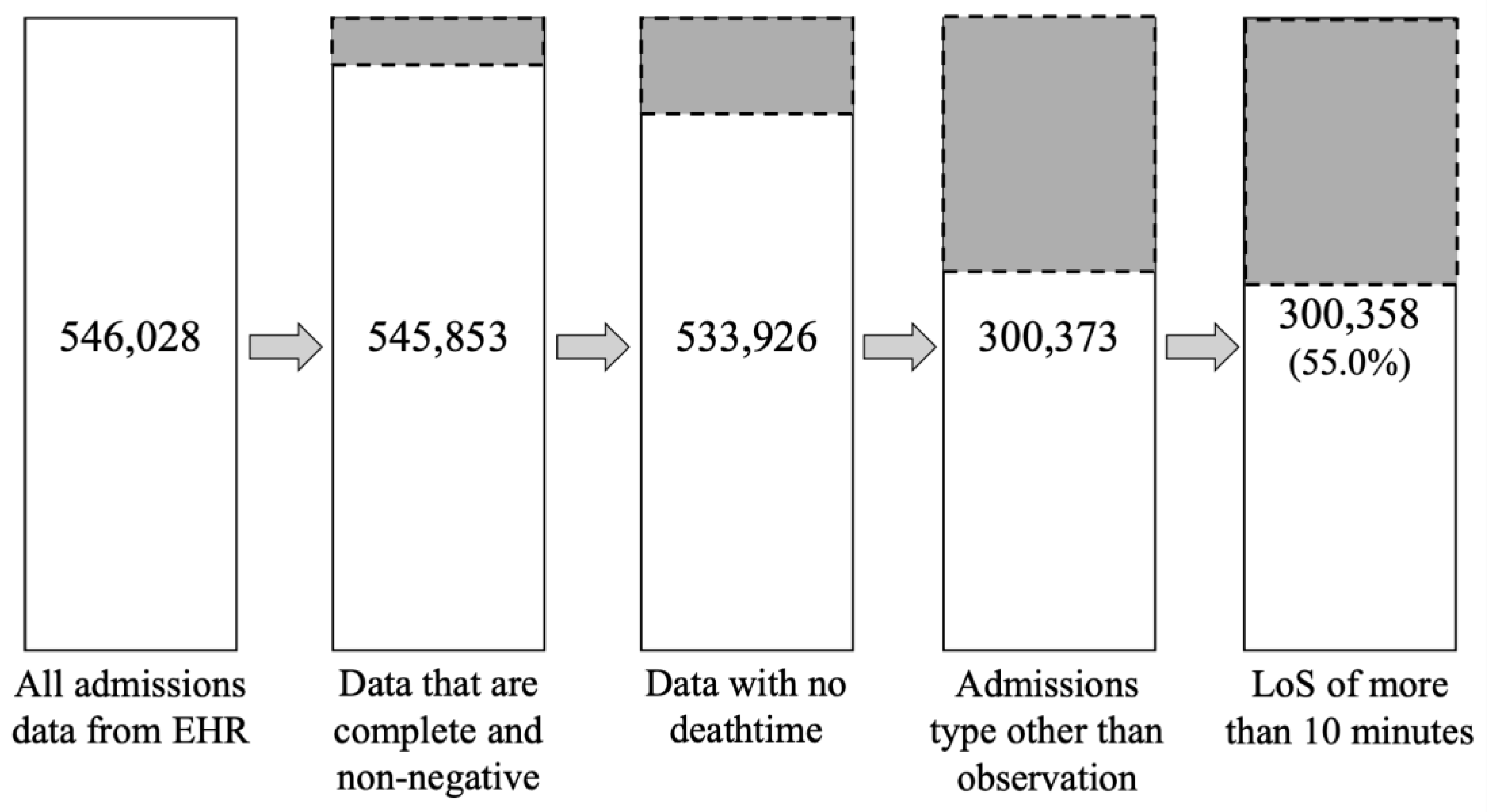
Figure 2.
Distribution of LoS in days (A) Full dataset. (B) Short-LoS between 2 hours and 5 days. (C) Long-LoS between 5 days and 28 days.
Figure 2.
Distribution of LoS in days (A) Full dataset. (B) Short-LoS between 2 hours and 5 days. (C) Long-LoS between 5 days and 28 days.
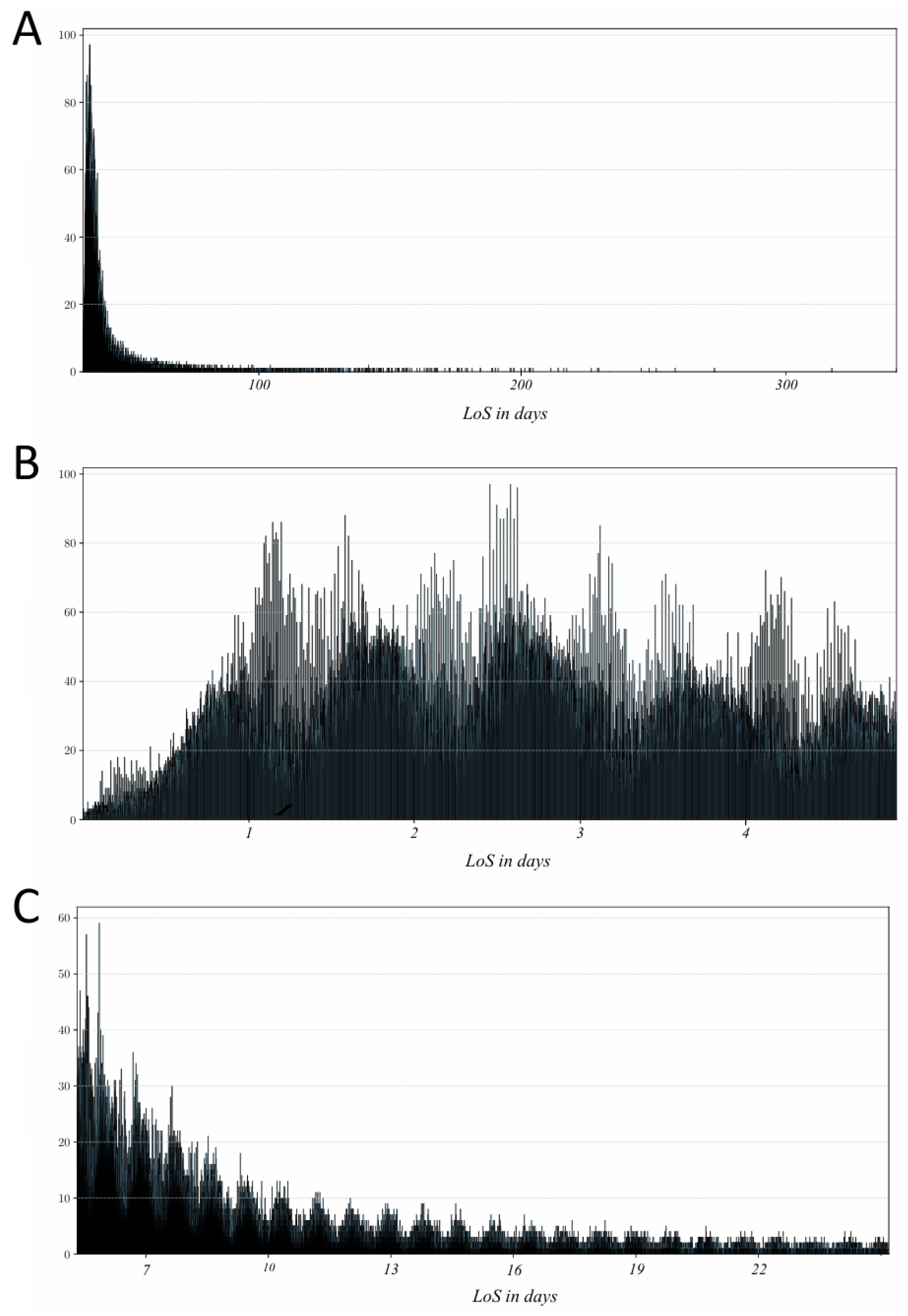
Figure 3.
Architecture of patient latent discoverer (left) and physician latent discoverer (right) in CDLD. The numbers in parentheses indicate the number of nodes in each layer. 'L2' denotes L2 normalization, 'BN' denotes batch normalization. The labels 'fixed' and 'update' above the feature and the latent indicate whether the parameters are frozen or updatable during training.
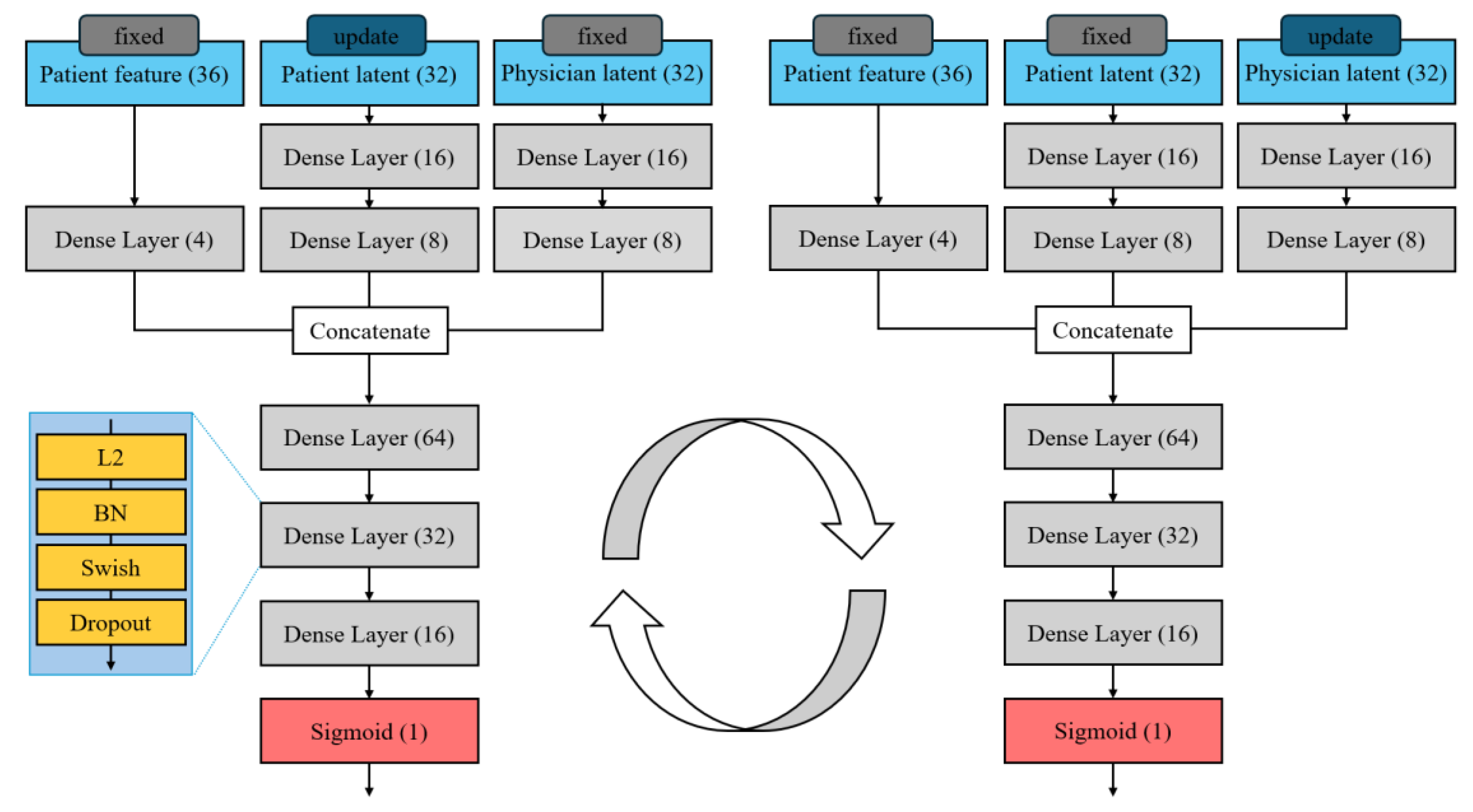
Figure 4.
RMSE per fold and loss reduction over epoch (fold-wise). The figures show consistent RMSE values across 10 folds.
Figure 4.
RMSE per fold and loss reduction over epoch (fold-wise). The figures show consistent RMSE values across 10 folds.
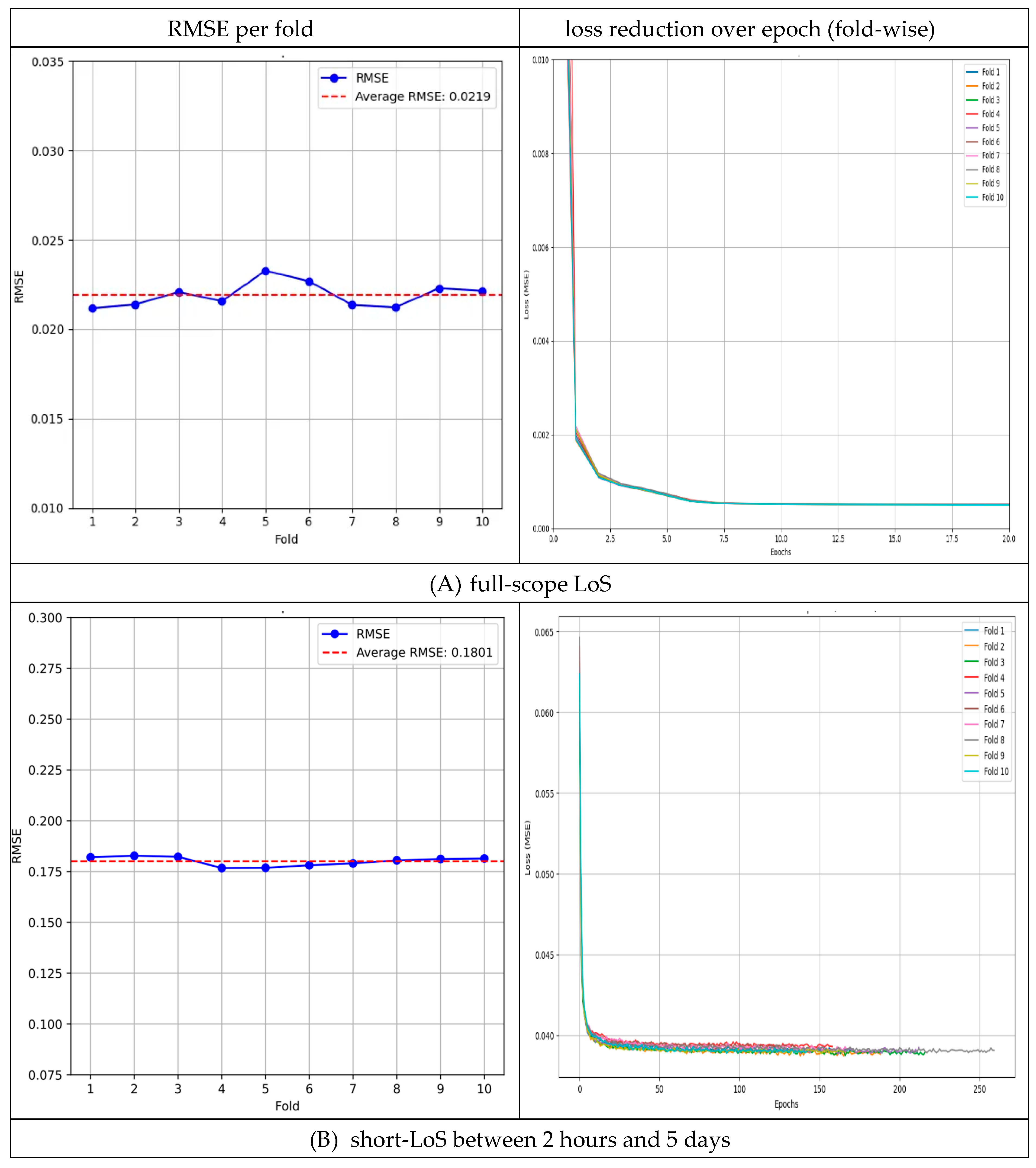
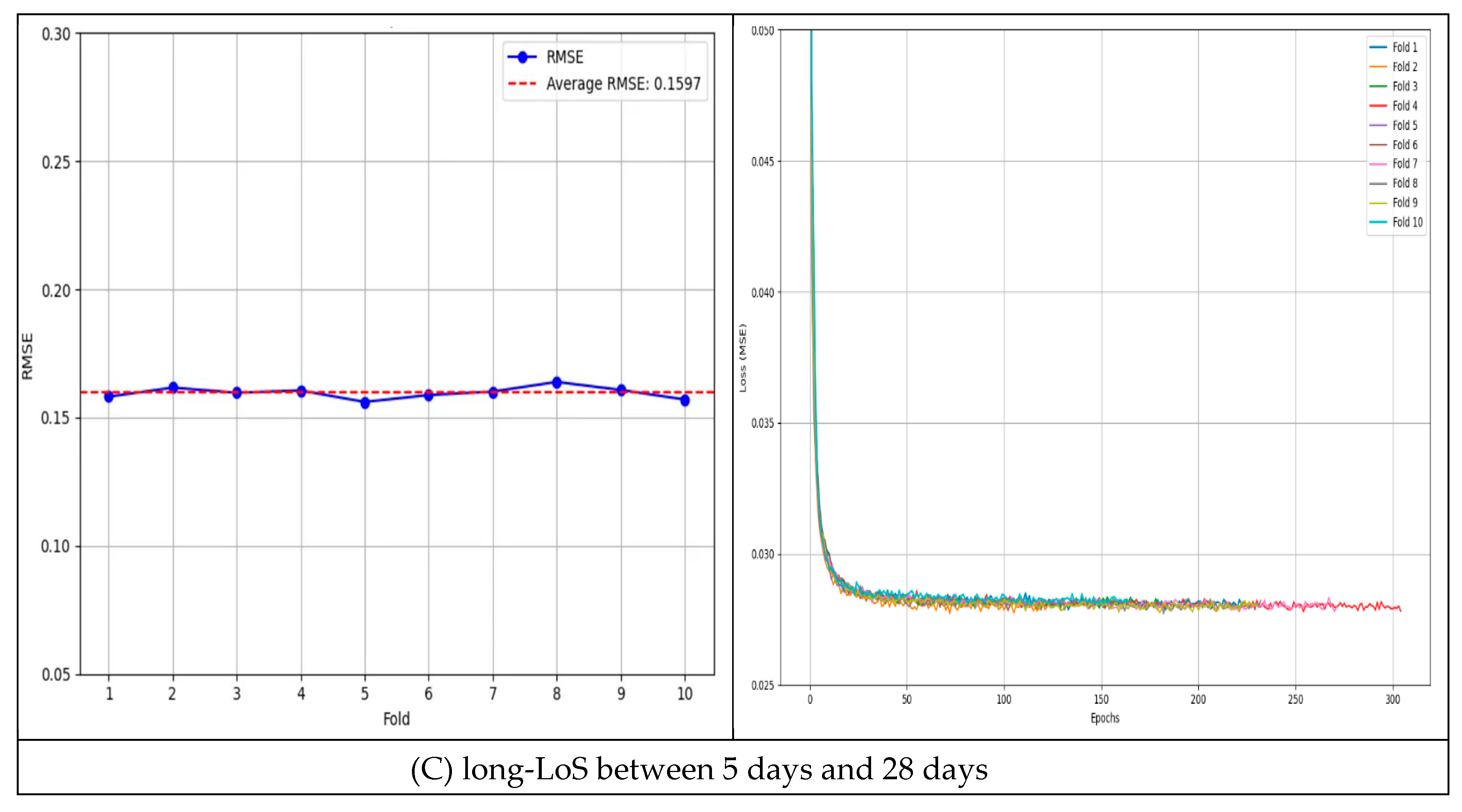
Figure 5.
The feature importance plot’s x-axis represents the mean (|SHAP value|), which indicates the average impact on the model output magnitude. The y-axis displays the top 20 most influential features ranked by their SHAP values.
Figure 5.
The feature importance plot’s x-axis represents the mean (|SHAP value|), which indicates the average impact on the model output magnitude. The y-axis displays the top 20 most influential features ranked by their SHAP values.
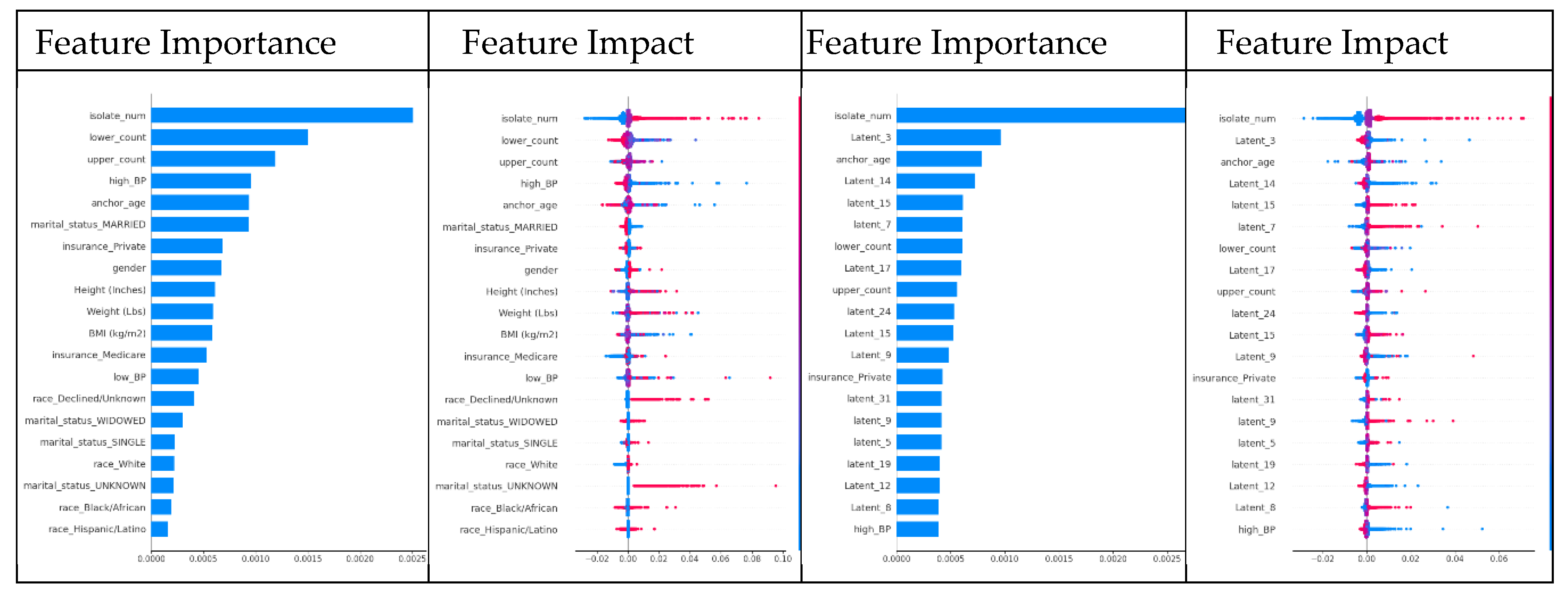
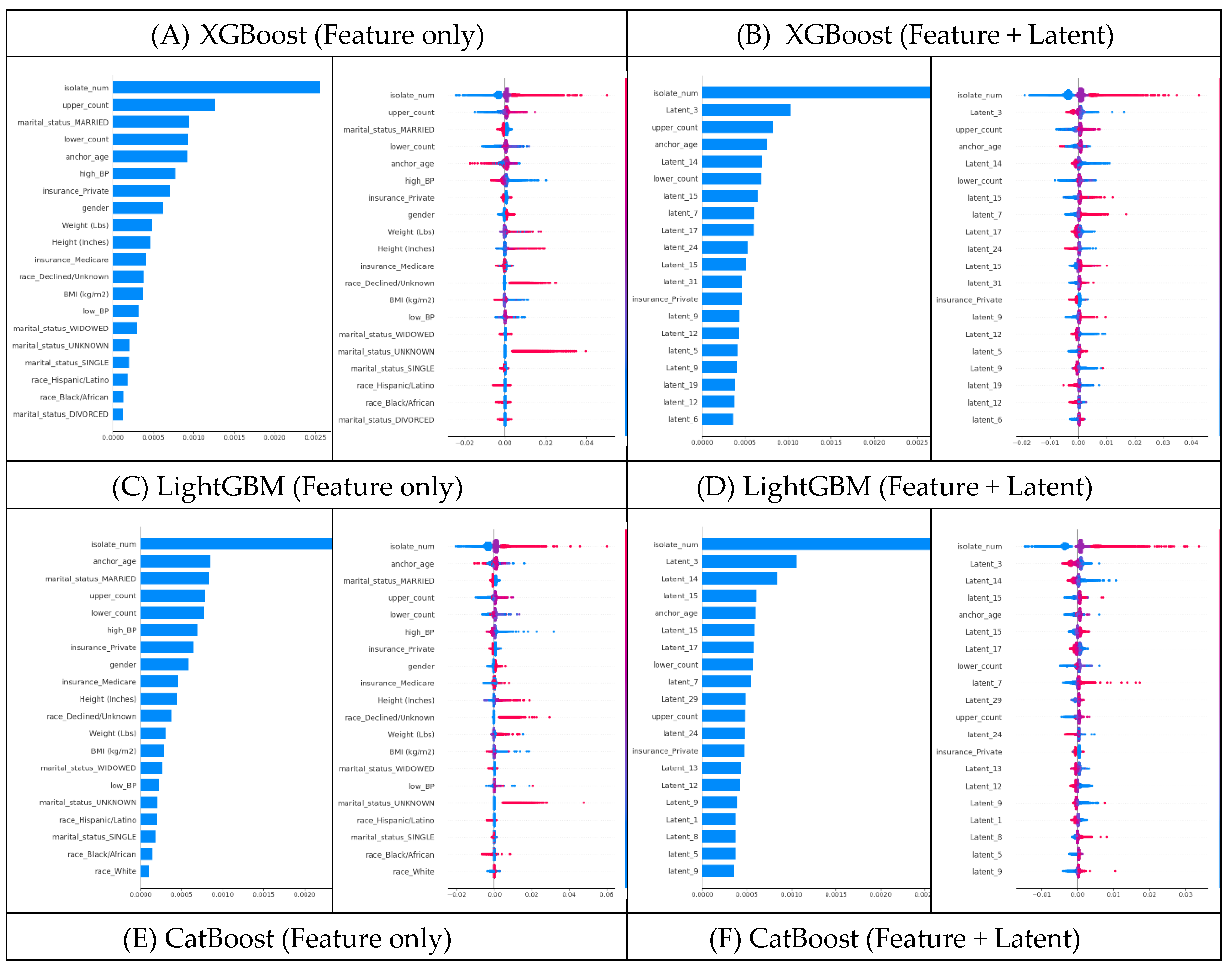

Table 1.
Patient entity features (merged from MIMIC-IV tables by subject_id) with categories and preprocessing details.
Table 1.
Patient entity features (merged from MIMIC-IV tables by subject_id) with categories and preprocessing details.
| Dataset | Columns | Count | Values |
| admissions.csv | insurance | 6 | 1. Medicaid, 2. Medicare, 3. Private, 4. Other, 5. No charge, 6. UNKNOWN |
| language | 29→8 | 1. ‘English’: ‘English’ 2. ‘Spanish-Portuguese’: ‘Spanish’, ‘Portuguese’ 3. ‘East Asia’: ‘Chinese’, ‘Japanese’, ‘Korean’ 4. ‘Southeast Asia’: ‘Vietnamese’, ‘Khmer’, ‘Thai’ 5. ‘Europe’: ‘Russian’, ‘French’, ‘Modern Greek (1453-)’, ‘Polish’, ‘Italian’, ‘Armenian’ 6. ‘Middle East Asia’: ‘Arabic’, ‘Persian’, ‘Hindi’, ‘Bengali’ 7. ‘Africa’: ‘Amharic’, ‘Somali’, ‘Haitian’, 8. ‘Other’: Others |
|
| marital_status | 5 | 1. WIDOWED, 2. MARRIED, 3. SINGLE, 4. DIVORCED, 5. UNKNOWN |
|
| race | 33→7 | 1. ‘White’: ‘WHITE’, ‘WHITE - RUSSIAN’, ‘WHITE - OTHER EUROPEAN’, ‘WHITE - BRAZILIAN’, ‘WHITE – EASTERN EUROPEAN’ 2. ‘Black/African’: ‘BLACK/AFRICAN AMERICAN’, ‘BLACK/CAPE VERDEAN’, ‘BLACK/AFRICAN’, ‘BLACK/CARIBBEAN ISLAND’ 3. ‘Asian’: ‘ASIAN’, ‘ASIAN - CHINESE’, ‘ASIAN - SOUTHEAST ASIAN’, ‘ASIAN - KOREAN’, ‘ASIAN - ASIAN INDIAN’ 4. ‘Hispanic/Latino’: ‘HISPANIC/LATINO - SALVADORAN’, ‘HISPANIC/LATINO - PUERTO RICAN’, ‘HISPANIC/LATINO - GUATEMALAN’, ‘HISPANIC/LATINO - DOMINICAN’, ‘HISPANIC/LATINO - MEXICAN’, ‘HISPANIC OR LATINO’, ‘HISPANIC/LATINO - CUBAN’, ‘HISPANIC/LATINO - HONDURAN’, ‘HISPANIC/LATINO - CENTRAL AMERICAN’, ‘HISPANIC/LATINO - COLOMBIAN, ‘SOUTH AMERICAN’ 5. ‘Native American’: ‘AMERICAN INDIAN/ALASKA NATIVE’ 6. ‘Multiple Race/Ethnicity’: ‘MULTIPLE RACE/ETHNICITY’ 7. ‘Declined/Unknown’: ‘UNKNOWN’, ‘UNABLE TO OBTAIN’, ‘PATIENT DECLINED TO ANSWER’, missing values |
|
| patients.csv | gender | 2 | Female: 0, Male: 1 |
| anchor_age | Normalized values (0-1 range) | ||
| microbiologyevents.csv | isolate_num | Normalized values (0-1 range) | |
| omr.csv | high_BP (mmHg) | Normalized mean values of ‘high_BP’, ‘high_BP_lying’, ‘high_BP_Sitting’, ‘high_BP_Standing’, ‘high_BP_1’, and ‘high_BP_3’ (0-1 range) | |
| low_BP (mmHg) | Normalized mean values of ‘low_BP’, ‘low_BP_lying’, ‘low_BP_Sitting’, ‘low_BP_Standing’, ‘low_BP_1’, and ‘low_BP_3’ (0-1 range) | ||
| BMI (kg/m2) | Normalized mean values (0-1 range) | ||
| height (inches) | Normalized mean values (0-1 range) | ||
| weight (Lbs) | Normalized mean values (0-1 range) |
Table 2.
RMSE and CV values for overall, short, and long-LoS.
| average RMSE | best RMSE | standard deviation RMSE | CV (%) | |
| full-scope LoS | 0.0219 | 0.0212 | 0.0007 | 3.18 |
| short-LoS between 2 hours and 5 days | 0.1801 | 0.1767 | 0.0023 | 1.25 |
| long-LoS between 5 days and 28 days | 0.1597 | 0.1561 | 0.0023 | 1.43 |
Table 3.
Simple DNN, XGBoost, LightGBM, and CatBoost model RMSE values comparing two datasets.
| feature only | feature and latent trait | decrease rate (%) | |
| simple DNN | 0.0228 | 0.0214 | 6.1404 |
| XGBoost | 0.0226 | 0.0217 | 3.9823 |
| LightGBM | 0.0226 | 0.0216 | 4.4248 |
| CatBoost | 0.0227 | 0.0218 | 3.9648 |
Disclaimer/Publisher’s Note: The statements, opinions and data contained in all publications are solely those of the individual author(s) and contributor(s) and not of MDPI and/or the editor(s). MDPI and/or the editor(s) disclaim responsibility for any injury to people or property resulting from any ideas, methods, instructions or products referred to in the content. |
© 2025 by the authors. Licensee MDPI, Basel, Switzerland. This article is an open access article distributed under the terms and conditions of the Creative Commons Attribution (CC BY) license (http://creativecommons.org/licenses/by/4.0/).
Copyright: This open access article is published under a Creative Commons CC BY 4.0 license, which permit the free download, distribution, and reuse, provided that the author and preprint are cited in any reuse.


