Submitted:
19 June 2025
Posted:
23 June 2025
You are already at the latest version
Abstract
Satellite imagery is crucial for monitoring global economic and ecological changes. However, integrating diverse datasets from different satellites is challenging due to differences in sensing technologies, lack of standardized calibration, and instrument hardware drift over time. Converting images from one sensor to another, like from WorldView-3 (WV) to SuperDove (SD), involves spectral band resampling and radiometric intensity scaling. A parametrized convolutional network approach has shown promise in non-linear conversion tasks across sensor domains, but it introduces artefacts when objects are in motion, due to temporal delays between multispectral band acquisitions. This results in spuriously blurred images of moving objects in the converted imagery. To resolve this, we propose an enhanced model, the Physics-Informed Gaussian-Enforced Separated-Band Convolutional Conversion Network (PIGESBCCN), which better accounts for spatial, spectral, and temporal correlations between bands.
Keywords:
physics-informed ML
; Bayesian optimization
; satellite image conversion
; scene simulation
1. Introduction
Satellite imagery can provide crucial benefits in tracking global economic and ecological changes. However, integrating diverse datasets from the myriads of observation satellites available poses significant challenges. Issues arise from differences in sensing technologies, the absence of standardized calibration methods prior to satellite launches, and changes in instruments over time. Although improved calibration techniques could enhance alignment of future data acquisition [1], a large amount of historical data remains mutually incompatible. For instance, the U.S. Geological Survey’s Global Fiducials Library combines Landsat images from 1972 with Sentinel-2 images from 2015 [2], highlighting the need for methods to effectively bridge different image types.
Converting satellite imagery from the domain of one sensor, such as WorldView-3 (WV), to another, such as SuperDove (SD), is non-trivial. As a first step, spectral resampling is necessary to translate the wavelength response of the WV sensor filters into the desired wavelengths of the SD image bands. However, the resampled image remains quantitatively and qualitatively divergent from an image truly acquired in SD space, so additional radiometric conversions are required. Building off previous windowed image regression tasks [3], we have demonstrated initial success with a parametrized convolutional neural network (PCNN) approach that leverages a Bayesian hyperparameter optimization loop to identify a performant model in this complex and often opaque conversion problem [4].
Though demonstrated to be qualitatively and quantitatively performant on converting stationary images, we identify spurious conversion artefacts with the PCNN approach when objects in the field of view are in motion. In these instances, the time delay between band acquisitions means that the moving object should appear localized in slightly different spatial locations across the bands, and a rainbow-like visual effect should be observed when viewing multiple bands at once (such as in a traditional RGB view) [5]. The issue arises because the previous PCNN model treats all image bands together in the prediction of a converted spectra, meaning that the effect of the moving object in each band spuriously bleeds over to every other band. This results in an expanded blurred blob for moving objects in the converted image, instead of spatiotemporally localized object signatures separated by band. Preserving these image features is of practical importance with object tracking applications to accurately represent where and at what time a moving object of interest appears.
Radiometrically accurate simulations of 3D objects and environments have been studied for decades. In particular, the Quick Image Display (QUID) model continually developed by Spectral Sciences, Inc. since the early 90s [6] incorporates six basic signature components including thermal surface emissions, scattered solar radiation, scattered earthshine, scattered skyshine, plume emission from hot molecular or particular species, and ambient atmospheric transmission/emission. QUID computes radiance images at animation rates by factoring thermal emission and reflectance calculations into angular and wavelength dependent terms. This factorization allows for the precomputation of wavelength-dependent terms which do not change with target-observer angles, enabling fast object rendering and scene simulation capabilities. As a result, QUID has found broad application as a general tool for moving object simulation, from ground-based automobiles [7] to aerial missiles [8].
To address this issue of correctly treating moving objects, here we introduce an expanded Physics-Informed Gaussian-Enforced Separated-Band Convolutional Conversion Network (PIGESBCCN) to handle known spatial, spectral, and temporal correlations between bands, and evaluate against QUID-simulated moving object scenes. Methods for data preparation, model optimization and evaluation, and for simulating imagery of moving target signatures labeled with ground truth data of object size and motion are discussed in the Materials and Methods section, followed by Results and Conclusions.
2. Materials and Methods
2.1. Dataset Curation
Satellite imagery of the same location in Turkey was acquired via both WV and SD sensors. WV images were acquired at spectral bands of 425, 480, 545, 605, 660, 725, 832, 950 nm. SD images were acquired at 443, 490, 531, 565, 610, 665, 705, 865 nm. WV images were band resampled to SD space using the open-source Spectral Python library, commonly used for processing hyperspectral image data [9]. After band resampling, labeled pairs of data were formed by taking matched pixel locations from the WV and SD images, and expanding a window around the WV location to obtain a region for convolutional input. Symmetric padding was used for windows at the periphery of the image. Of these WV/SD pairs, 70% were used as training data, 20% as validation data, and 10% reserved as testing data for a total of 2,303,417 training data pairs, 658,119 validation data pairs, and 329,060 test data pairs.
2.2. Hyperparameter Tuning for Model Optimization
The neural network was implemented in Python using the PyTorch library [10] and parametrized for application of automated hyperparameter tuning workflows. Here we utilize the Adaptive Experimentation Platform (Ax) [11] for Bayesian optimization of hyperparameters. Specifically, for the surrogate function we use the commonly implemented Gaussian process, and for the acquisition function we use expected improvement as shown in Equations 1 and 2:
where f’ is the minimal value of f observed so far, u(x) is the utility of choosing f(x), D are the set of previous observations and E is the expected value function. The search space of hyperparameters treated here is defined as below:
- Gaussian blur size: a range of integers from 3 to 10, inclusive
- Window size: a range of integers from 3 to 20, inclusive
- Kernel size: a choice of integers between 3 and 5
- Pooling mode: a choice of modes between average and max
- Learning rate: a range of floats from 0.0001 to 0.01, inclusive
- Batch size: a choice of integers between 256, 512, 1024, and 2048
As a result of this process, we identify an optimized PIGESBCCN model with hyperparameters of blur size 6, window size 14, kernel size 5, average pooling mode, learning rate 0.00076, and batch size 256, for a total model size of 15,752 parameters.
While the training loss is minimized via direct parameter training and validation loss is minimized via hyperparameter tuning, the test set comprises data that the model has never seen. Importantly, our optimized model performs well on the test set, with 1) test error distributions in family with both training and validation, and 2) parity plots with r-squared values >0.96 across every band, as shown in the following Figure 1.
2.3. Spectral Angle Deviation Calculation
Spectral angles quantify the similarity between spectra, with smaller angles reflecting greater similarity. This is determined by measuring the angle between vectorized spectra in N-dimensional space [12], where the images in this study consist of N=8 bands. To assess the performance of the ML conversion process, we compute the WV-to-SD deviation for both pre- and post-ML converted WV. The spectral angle α is then calculated using the formula provided in Equation 3:
for each co-registered pixel location in a pair of WV and SD images with WV spectra , and SD spectra . We can then plot heatmaps of these spectral angles to highlight locations of high deviance, as in Figure 4.
2.4. QUID Target Simulations
The QUID scene simulation method employs 3D wireframe models attributed with spectral bidirectional reflectance distribution functions (BRDFs) to characterize the reflective/emissive properties of the object surfaces and incorporate atmospheric simulations from MODTRAN 6 [13]. The environmental illumination from the sun and other sources includes the solar and diffuse fluxes necessary to illuminate the ground, a cloud field, and a target viewed through any line-of-sight through the atmosphere. The data also defines the path radiance and transmittance to model the opacity and brightness of the atmosphere between a sensor and a target. The current capabilities can compute accurate intensity images of targets in wavelengths from 0.4 µm to 15 µm. Our simulation approach separates in-band spectral quantities from angular factors to provide scene simulation rates of hundreds of hertz on a desktop workstation.
Using this software we simulated a black sport utility vehicle (SUV) at sea level, moving toward a heading of 123.3° south of east (for a southwest direction) at 13 m/s (29 mph). The sun was placed at a solar azimuth angle of 164.0° and a solar elevation angle of 0°. The black SUV was simulated across 8 spectral bands, Coastal Blue (443 nm), Blue (490 nm), Green 1 (531 nm), Green 2 (565 nm), Yellow (610 nm), Red (665 nm), Red Edge (705 nm), and NIR (865 nm). Importantly however, these bands were temporally acquired in the order of Blue, Red, Green 1, Green 2, Yellow, Red Edge, NIR, Coastal Blue, with timing matching SD imagery. As a result, the output QUID-simulated scene exhibits band localized SUV locations consistent with a true SD acquisition.
3. Results
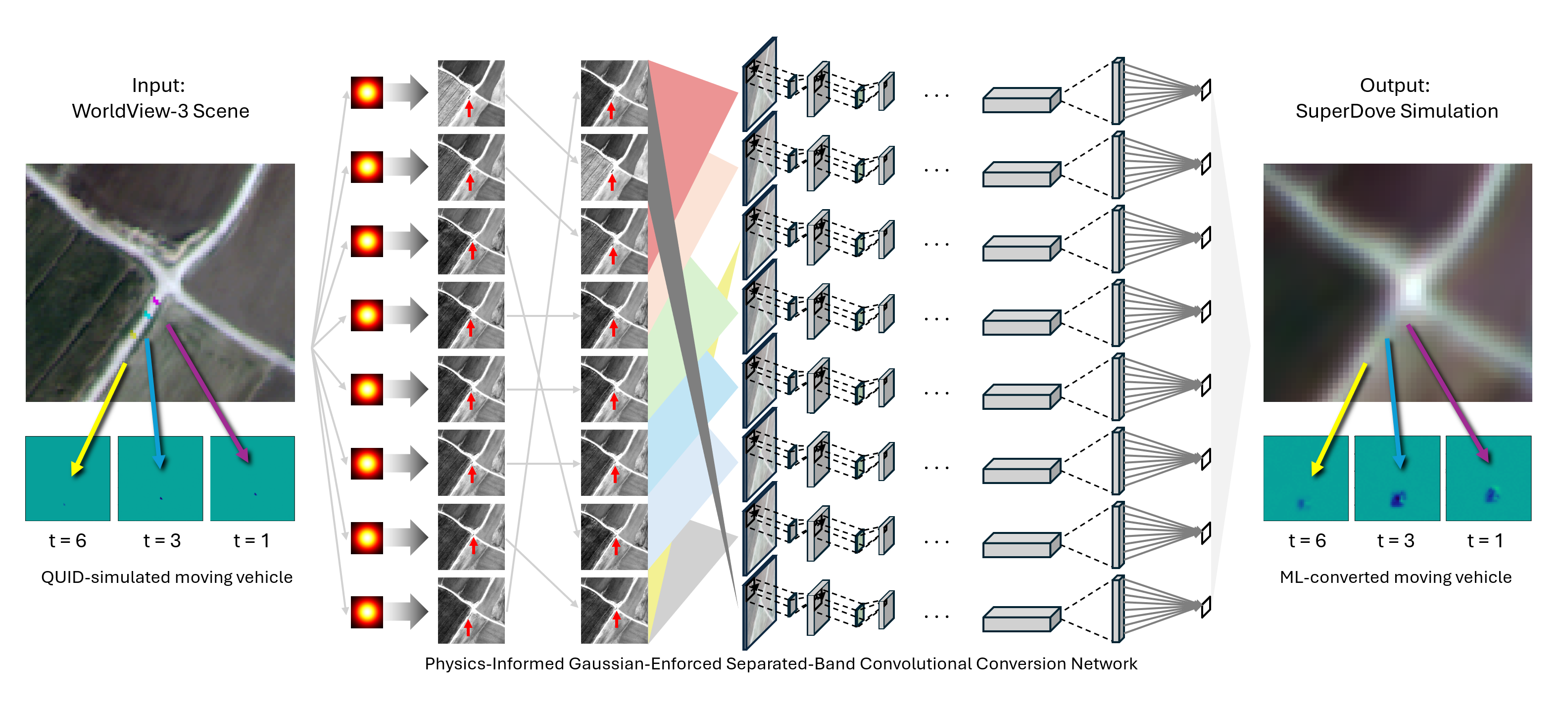
The PIGESBCCN model architecture, as shown in Figure 2, first separates out each band of the input image with band-specific Gaussian blurs derived from analysis of identical contrast targets in both the WV (input) and SD (output) domains. We then rearrange the order of the input scene bands by temporal acquisition. Once reordered, we chunk the image into 8 temporally adjacent 3-band sections to physically encode temporal relationships into the model architecture. The first and last chunks at the temporal periphery repeat their earliest and latest bands, respectively, to yield 3-band chunks the same shape as temporally internal chunks. After sectioning, these temporal chunks are then rearranged back into the original spectral ordering. Then, each of the 8 3-band chunks are fed through separate parameterized convolutional network paths to obtain a prediction for each band, and ultimately a converted spectra for each pixel of the input image.
Two images capturing the same spatial location—a scene in Turkey—were obtained using the WV and SD sensors, respectively. The spectra in the SD image are used to label their respective WV regions, constituting a paired dataset to facilitate learning the relationship between the WV and SD spectra. Due to the differing intensity scales of the WV and SD images (0-255 for WV and 0-24545 for SD), we first normalize the pixel values of each image to a range of 0 to 1 by dividing by the maximum value of the image. After normalization, we split the pixels from these images into training, validation, and test datasets using a 70-20-10 split. Further details are provided in the Materials and Methods section.
The training set is employed for direct parameter training. Then, as in previous work [14], we employ an automated hyperparameter tuning process using Bayesian optimization. The validation set guides the hyperparameter tuning loop, ultimately resulting in a final model that minimizes both training and validation loss. The paired WV and SD scenes used for training and the loss curves for the optimized model are shown in Figure 3. Details on hyperparameter tuning and optimized model performance are provided in the Materials and Methods section.
To quantify the effectiveness of ML spectral conversion, we present the spectral angle deviations from actual SD spectra in Figure 4. Details of the calculation are in the Materials and Methods section. Panel a compares spectral angle deviations from SD to the WV image after simple band resampling, while panel b compares from SD to the WV image converted with the trained ML model. In this visualization, brighter pixels represent greater deviations. The predominantly dark image in panel b indicates that the ML converted image is significantly closer to the actual SD data compared to simple band resampling. A horizontal trace across the field of view indicates that the average spectral angle deviation along that trace is 5.12° for the WV image after band resampling, which decreases significantly to an average of just 1.42° following conversion with the trained ML model.
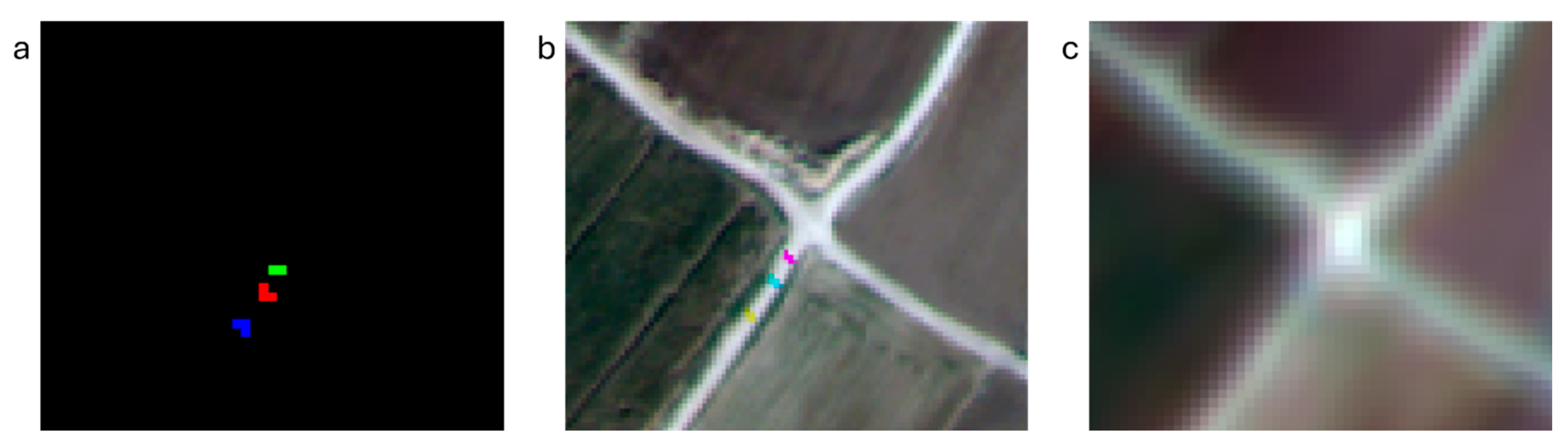
Now, we utilize QUID to simulate a moving object in the input WV scene. Here, we specifically simulate a black SUV, as a representative generic target that can be found on an urban highway. Note, that due to the time delay between band acquisitions, the moving object appears as a “rainbow” in a visible color image as it traverses in space. As the SUV in question is black, these colors then appear inverted when on a bright grey road background – masking the respective color band from the background. The QUID-simulated object scene is then passed through our PIGESBCCN model and converted to SD space to evaluate how well the ML conversion preserves band-separated object locations, as shown in the following Figure 5. Details of the target simulation are provided in the Materials and Methods section.
Figure 4.
Spectral angle deviation maps for a. WV band resampled image vs. SD baseline and the b. ML converted image vs. SD baseline. c. The average spectral angle difference across a sample horizontal profile decreases from 5.12° to 1.42° after ML conversion.
Figure 4.
Spectral angle deviation maps for a. WV band resampled image vs. SD baseline and the b. ML converted image vs. SD baseline. c. The average spectral angle difference across a sample horizontal profile decreases from 5.12° to 1.42° after ML conversion.
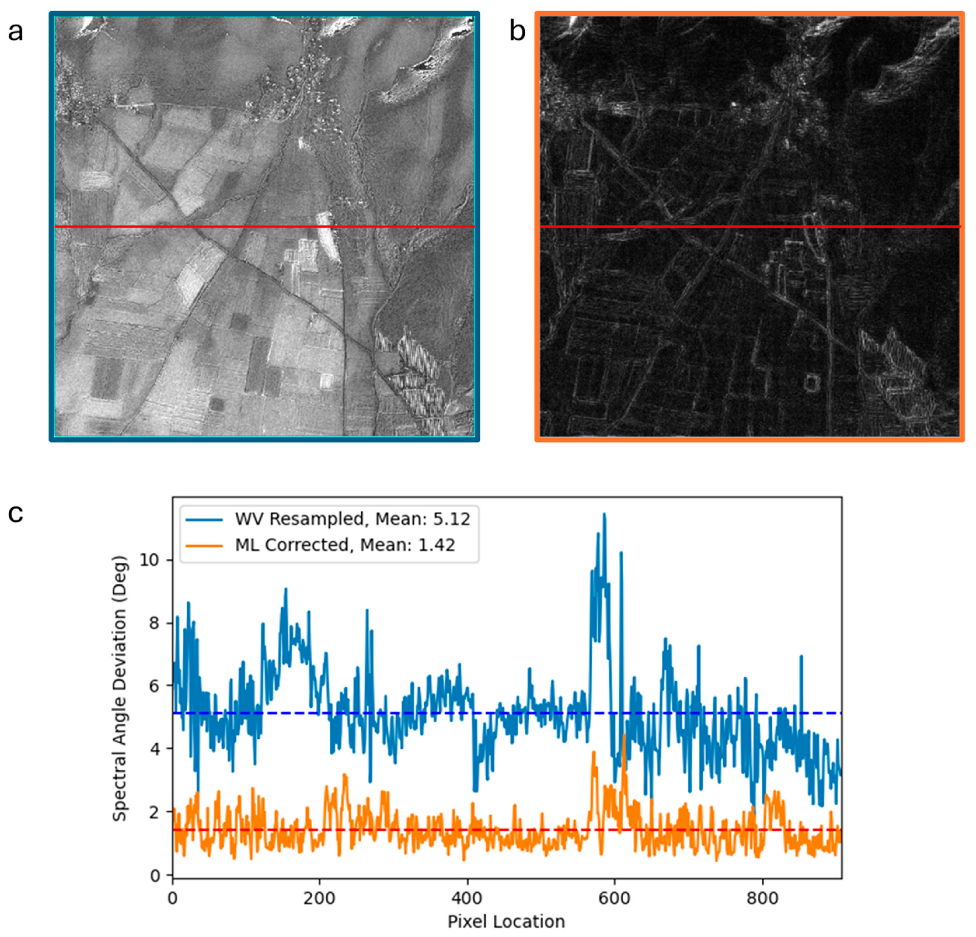
Figure 5.
QUID-simulated black SUV at a roadway intersection with a. object mask showing the location of the SUV in the RGB bands. This manifests as b. reversed colors when the black SUV is simulated on a bright grey road. This scene is then converted from WV to c. SD imagery via the PIGESBCCN model, where the rainbow effect is faint – but crucially still present.
To evaluate the ML model performance on converting a moving object to SD space, we use a simple Gaussian blur of the WV QUID images, both with and without a moving target, as a comparative baseline. This blur serves to simulate the difference in spatial resolution between the WV and SD sensors while maintaining correctly band-separated object locations. Specifically, using band-dependent full width half maximums of 4.258, 4.268, 4.267, 4.250, 4.284, 4.439, 4.203, and 4.363, for spectral bands of 0.443 nm, 0.490 nm, 0.531 nm, 0.565 nm, 0.610 nm, 0.665 nm, 0.705 nm, and 0.865 nm respectively. We then pass the same WV QUID images through the PIGESBCCN ML conversion model. Finally, we subtract out the blurred background from the blurred background plus target image to isolate the effect on the target, as shown in Figure 6.
Zooming in on the target in a particular band allows us to qualitatively compare the difference between the ML conversion and baseline Gaussian blurring. Here, an example focusing on band 4 is shown in the third column of Figure 6. The ML converted target qualitatively appears with a similar location and size as the Gaussian blurred target. Note that the color of the ML converted target is not the same as the baseline blurred target. This is to be expected, as the baseline blurred target remains in WV color space while the ML converted target is in simulated SD color space.
We then conduct background subtraction for each of the 8 bands and use a value threshold of 5% to mask the target from the background. Then, comparing the baseline Gaussian blurred target and the ML converted target allows us to visualize the deviation between the ML method and baseline procedure for each band, as shown in Figure 7. First, this band-by-band visualization confirms proper target localization with slightly different spatial locations per band. Second, we see that these target locations for each band qualitatively align between the ML method and baseline blurring.
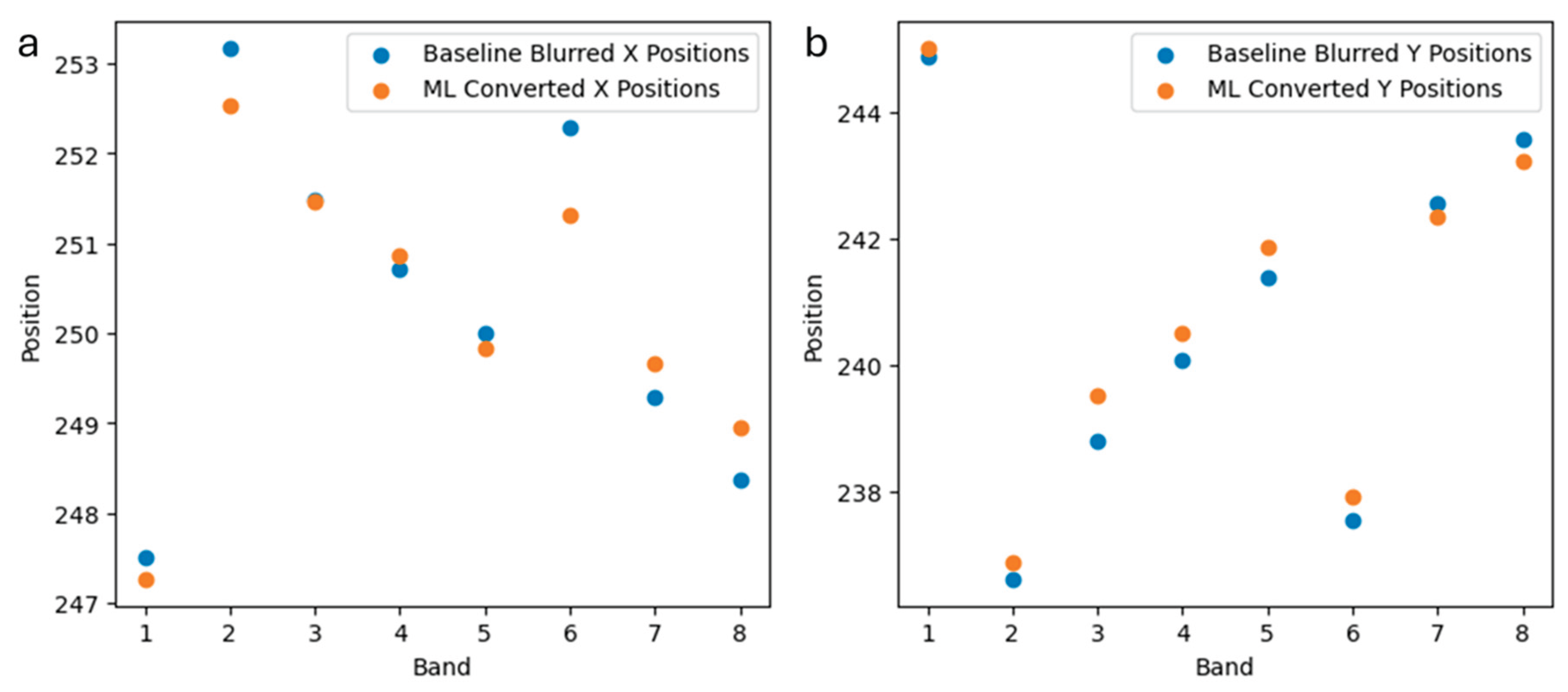
To quantitatively investigate the possibility of systematic errors associated with ML conversion, we compare target locations between the ML converted and baseline Gaussian approaches in Figure 8. Here, we see that the ML conversion yields target locations with good agreement to the baseline approach. Specifically, averaged locations for x and y coordinates yield deviations of only 0.12 and 0.23 pixels, respectively, between ML converted and baseline targets. This subpixel location accuracy indicates that the ML conversion successfully preserves target location without introducing systematic spatial translation errors. Furthermore, the averaged target size is only 1.6 pixels larger for the ML converted imagery (77 pixels) than the Gaussian blur baseline (75.4 pixels).
4. Discussion and Conclusions
ML models can successfully learn complex non-linear relationships to convert one data domain to another. Application to satellite imagery can allow greater usage of data from disparate sources for combined studies.
Correct treatment of moving targets within satellite imagery was identified as a key mode for improvement over previous PCNN models, requiring a more sophisticated approach. Leveraging known physical relationships of the problem domain to put specific structure and guiderails on model architecture allows for corrected performance. Specifically, band-dependent blurring, temporal reordering and chunking, and separated band specific prediction branches allows for improved treatment of spatial, temporal, and spectral characteristics.
As a result, the ML conversion approach detailed in this work operates quantitatively not only on stationary backgrounds but also for moving targets. The PIGESBCCN model enables accurate spectral conversion between WV and SD sensors, while maintaining moving target sizes and target locations across bands. Preservation of band localized moving targets is critical for moving target detection algorithms, a major application of satellite imagery data.
Future work may involve expanding into other image sensors and spectral bands, increasing computational efficiency for real-time conversion operations, and integrating our model architecture within live, periodic model training workflows for continually improved performance as more satellite imagery is acquired over time.
Author Contributions
Conceptualization, A.J.L. and R.S.; methodology, A.J.L. E.B, P.C, and T.P.; software, A.J.L. and T.P.; validation, A.J.L., T.P., P.C.; formal analysis, A.J.L.; investigation, A.J.L.; resources, R.S.; data curation, A.J.L. and R.S.; writing—original draft preparation, A.J.L.; writing—review & editing, A.J.L., T.S., E.B., P.C., and R.S.; visualization, A.J.L.; supervision, R.S.; project administration, R.S.
Funding
Support for this effort was funded under Air Force Research Laboratory Contract FA9453-21-C-0026. The views expressed are those of the author and do not necessarily reflect the official policy or position of the Department of the Air Force, the Department of Defense, or the U.S. government.
Data Availability Statement
The original contributions presented in this study are included in the article. Further inquiries can be directed to the corresponding author.
Conflicts of Interest
The authors declare no conflicts of interest.
Abbreviations
The following abbreviations are used in this manuscript:
| WV | WorldView-3 |
| SD | SuperDove |
| ML | Machine Learning |
| PIGESBCCN | Physics-Informed Gaussian-Enforced Separated-Band Convolutional Conversion Network |
| PCNN | Parameterized Convolutional Neural Network |
| QUID | QUick Image Display |
| SUV | Sport Utility Vehicle |
References
- G. Chander, T. J. Hewison, N. Fox, X. Wu, X. Xiong and W. J. Blackwell, “Overview of intercalibration of satellite instruments,” IEEE Transactions on Geoscience and Remote Sensing 51, no. 3, pp. 1056-1080, 2013.
- G. B. Fisher, E. T. Slonecker, S. J. Dilles, F. B. Molnia and K. M. Angeli, “Using Global Fiducials Library High-Resolution Imagery, Commercial Satellite Imagery, Landsat and Sentinel Satellite Imagery, and Aerial Photography to Monitor Change at East Timbalier Island, Louisiana, 1953–2021,” Core Science Systems and the National Civil Applications Center, 2023.
- A. J. Lew, C. A. Stifler, A. Cantamessa, A. Tits, D. Ruffoni, P. U. Gilbert and a. M. J. Buehler, “Deep learning virtual indenter maps nanoscale hardness rapidly and non-destructively, revealing mechanism and enhancing bioinspired design,” Matter, vol. 6, no. 6, pp. 1975-1991, 2023.
- A. J. Lew, E. Brewer, T. Perkins, P. Corlies, J. Grassi, J. Marks, A. Friedman, L. Jeong and R. Sundberg, “Enhancing Cross-Sensor Data Integration through Domain Conversion of Satellite Imagery with Hyperparameter Optimized Machine Learning,” Algorithms, Technologies, and Applications for Multispectral and Hyperspectral Imaging XXXI. SPIE, 2025.
- E. Keto and W. Andres Watters, “Detection of Moving Objects in Earth Observation Satellite Images: Verification,” arXiv:2406.13697 [astro-ph.EP], pp. 1-7, 2024. [CrossRef]
- R. L. Sundberg, J. Gruninger, M. Nosek, J. Burks and E. Fontaine, “Quick image display (QUID) model for rapid real-time target imagery and spectral signatures,” Technologies for Synthetic Environments: Hardware-in-the-Loop Testing II. SPIE, vol. 3084, pp. 272-281, 1997.
- R. Sundberg, S. Adler-Golden, T. Perkins and K. Vongsy, “Detection of spectrally varying BRDF materials in hyperspectral reflectance imagery,” 2015 7th Workshop on Hyperspectral Image and Signal Processing: Evolution in Remote Sensing (WHISPERS), pp. 1-4, 2015.
- T. Perkins, R. Sundberg, J. Cordell, Z. Tun and M. Owen, “Real-time target motion animation for missile warning system testing,” Proc. SPIE, vol. 6208, pp. 1-12, 2006.
- V. Tiwari, V. Kumar, K. Pandey, R. Ranade and S. Agarwal, “Simulation of the hyperspectral data from multispectral data using Python programming language,” Multispectral, Hyperspectral, and Ultraspectral Remote Sensing Technology, Techniques and Applications VI. SPIE, vol. 9880, pp. 203-211, 2016.
- A. Paszke, S. Gross, F. Massa, A. Lerer, J. Bradbury, G. Chanan, T. Killeen, Z. Lin and N. Gimelshein, “PyTorch: An Imperative Style, High-Performance Deep Learning Library,” arXiv:1912.01703 [cs.LG], 2019.
- Meta Platforms, Inc., “Adaptive Experimentation Platform,” 2024. [Online]. Available: https://github.com/facebook/Ax.
- F. A. Kruse, A. B. Lefkoff and J. W. Boardoman, “The Spectral Image Processing System (SIPS)- Interactive Visualization and Analysis of Imaging Spectrometer Data,” Remote Sensing of Environment, © Elsevier publishing co. Inc., pp. 145-163, 1993.
- A. Berk, P. Conforti, R. Kennett, T. Perkins, F. Hawes and J. van den Bosch, “MODTRAN6: a major upgrade of the MODTRAN radiative transfer code,” in SPIE Defense and Security, 90880H, International Society for Optics and Photonics, 2014. [CrossRef]
- A. J. Lew, “A Brief Survey of ML Methods Predicting Molecular Solubility: Towards Lighter Models via Attention and Hyperparameter Optimization,” Preprints, no. 2024090849, 2024.
Figure 1.
Error histograms and parity plots for ML converted WV vs real SD spectral intensities per band, illustrating both 1) agreement between training, validation, and test sets and 2) accurate test predictions with r-squared values >0.96.
Figure 1.
Error histograms and parity plots for ML converted WV vs real SD spectral intensities per band, illustrating both 1) agreement between training, validation, and test sets and 2) accurate test predictions with r-squared values >0.96.
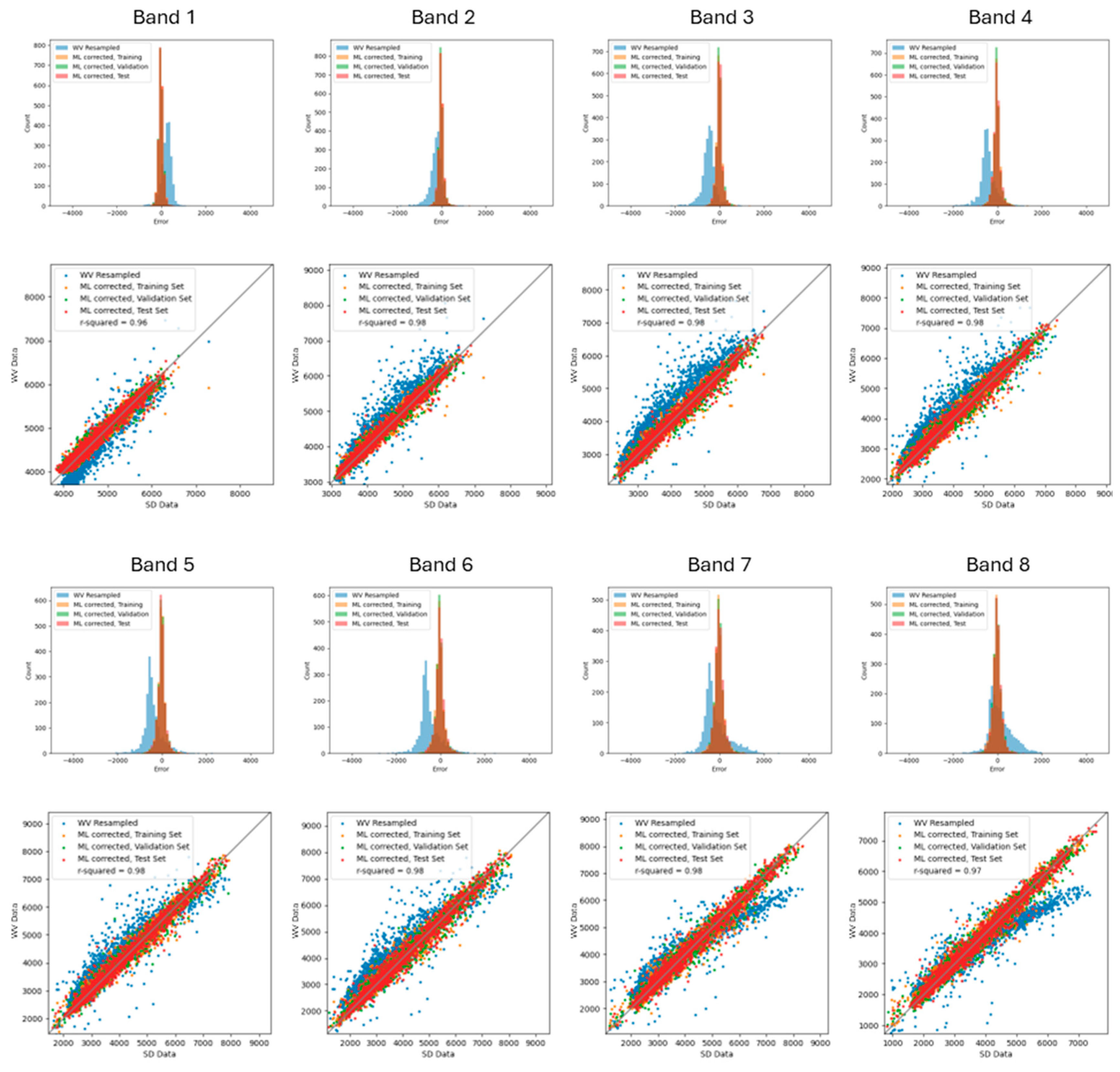
Figure 2.
PIGESBCCN incorporates physics-informed Gaussian blurring, band rearrangement, temporally adjacent band chunking, and separated band prediction branches to better encode known spatial, temporal, and spectral relationships into the model architecture. (Satellite Imagery Credit: ©2024 Maxar/NextView License).
Figure 3.
a. Spatially matched WorldView-3 (©2024 Maxar/NextView License) and SuperDove (©2024 Planet Labs PBC, USG Plus) imagery of a scene in Turkey used to train PIGESBCCN. b. Training and validation loss curves of hyperparameter optimized PIGESBCCN model.
Figure 3.
a. Spatially matched WorldView-3 (©2024 Maxar/NextView License) and SuperDove (©2024 Planet Labs PBC, USG Plus) imagery of a scene in Turkey used to train PIGESBCCN. b. Training and validation loss curves of hyperparameter optimized PIGESBCCN model.
Figure 6.
Taking a QUID image pair with and without a black SUV allows us to isolate the ML conversion model’s effect on the target and subsequently compare that effect to a baseline Gaussian blur.
Figure 6.
Taking a QUID image pair with and without a black SUV allows us to isolate the ML conversion model’s effect on the target and subsequently compare that effect to a baseline Gaussian blur.
Figure 7.
Per band comparison of target ML conversion and baseline Gaussian blurring.
Figure 8.
Quantitative agreement in a. x coordinate target locations and b. y coordinate target locations between ML conversion and baseline blurring.
Figure 8.
Quantitative agreement in a. x coordinate target locations and b. y coordinate target locations between ML conversion and baseline blurring.
Disclaimer/Publisher’s Note: The statements, opinions and data contained in all publications are solely those of the individual author(s) and contributor(s) and not of MDPI and/or the editor(s). MDPI and/or the editor(s) disclaim responsibility for any injury to people or property resulting from any ideas, methods, instructions or products referred to in the content. |
© 2025 by the authors. Licensee MDPI, Basel, Switzerland. This article is an open access article distributed under the terms and conditions of the Creative Commons Attribution (CC BY) license (http://creativecommons.org/licenses/by/4.0/).
Copyright: This open access article is published under a Creative Commons CC BY 4.0 license, which permit the free download, distribution, and reuse, provided that the author and preprint are cited in any reuse.


