
Submitted:
18 June 2025
Posted:
19 June 2025
You are already at the latest version
Abstract
Drawing inspiration from our human brain that designs different neurons for different tasks, recent advances in deep learning have explored modifying a network's neurons to develop so-called task-driven neurons. Prototyping task-driven neurons (referred to as NeuronSeek) employs symbolic regression (SR) to discover the optimal neuron formulation and construct a network from these optimized neurons. Along this direction, this work replaces symbolic regression with tensor decomposition (TD) to discover optimal neuronal formulations, offering enhanced stability and faster convergence. Furthermore, we establish theoretical guarantees that modifying the aggregation functions with common activation functions can empower a network with a fixed number of parameters to approximate any continuous function with an arbitrarily small error, providing a rigorous mathematical foundation for the NeuronSeek framework. Extensive empirical evaluations demonstrate that our NeuronSeek-TD framework not only achieves superior stability, but also is competitive relative to the state-of-the-art models across diverse benchmarks. The code is available at https://github.com/HanyuPei22/NeuronSeek.
Keywords:
Neuronal diversity
; tensor decomposition
; task-driven neuron
; super-expressive
1. Introduction
Deep learning has achieved significant success in a wide range of fields [1,2]. Credits for these accomplishments largely go to the so-called scaling law, wherein fundamental computational units such as convolutions and attention mechanisms are designed and scaled per an optimized architecture. Prominent examples include ResNet [3], Transformer [4], and Mamba [5]. Recently, motivated by neuroscience’s paramount contributions to AI, an emerging field called NeuroAI has garnered significant attention, which draws upon the principles of biological circuits in the human brain to catalyze the next revolution in AI [6]. The ambitious goal of NeuroAI is rooted in the belief that the human brain, as one of the most intelligent systems, inherently possesses the capacity to address complex challenges in AI development [7]. Hence, it can always serve as a valuable source of inspiration for guiding practitioners, despite the correspondence between biological and artificial neural networks sometimes being implicit.
Following NeuroAI, let us analyze the scaling law through the lens of brain computation. It is seen that the human brain generates complex intellectual behaviors through the cooperative activity of billions of mutually connected neurons with varied morphologies and functionalities [8]. This suggests that the brain simultaneously benefits from scale at the macroscopic level and neuronal diversity at the microscopic level. The latter is a natural consequence of stem cells’ directed programming in order to facilitate the task-specific information processing. Inspired by this observation, extensive research has shown that incorporating neuronal diversity into artificial neural networks can markedly enhance their capabilities [7]. For instance, researchers have transitioned beyond traditional inner-product neurons by integrating diverse nonlinear aggregation functions, such as quadratic neurons [9], polynomial neurons [10], and dendritic neurons [11]. Such networks have achieved superior performance in tasks like image recognition and generation, underscoring the promise and practicality of innovating a neural network at the neuronal level.
Along this direction, driven by the task-specific nature of neurons in our brain, recent research [12] introduced a systematic framework for task-driven neurons. Hereafter, we refer to prototyping task-driven neurons as NeuronSeek. This approach assumes that there is no single type of neurons that can perform universally well. Therefore, it enables neurons to be tailored for specific tasks through a two-stage process. As shown in Figure 1, in the first stage, the vectorized symbolic regression (SR)—an extension of symbolic regression [13,14] that enforces uniform operations for all variables—identifies the optimal homogeneous neuronal formula from data. Unlike traditional linear regression and symbolic regression, the vectorized SR searches for coefficients and homogeneous formulas at the same time, which can facilitate parallel computing. In the second stage, the derived formula serves as the neuron’s aggregation function, with learnable coefficients. Notably, activation functions remain unmodified in task-driven neurons. At the neuronal level, task-driven neurons are supposed to have superior performance than those one-size-fits-all units do, as it imbues the prior information pertinent to the task. More favorably, task-driven neurons can still be connected into a network to fully leverage the power of connectionism. Hereafter, we refer to task-driven neurons using symbolic regression as NeuronSeek-SR. NeuronSeek considers in tandem neuronal importance and scale. From design to implementation, it systematically integrates three cornerstone AI paradigms: behaviorism (the genetic algorithm runs symbolic regression), symbolism (symbolic regression distills a formula from data), and connectionism.
Despite this initial success, the following two major challenges remain unresolved in prototyping task-driven neurons.
- Non-deterministic and unstable convergence. While symbolic regression employs modified genetic programming (GP) to discover polynomial expressions [15,16], its tree-based evolutionary approach struggles to converge in high-dimensional space. The resulting formulas demonstrate acute sensitivity to certain hyperparameters, such as initialization conditions, population size, and mutation rate. This may confuse users about whether the identified formula is truly suitable for the task or due to the random perturbation, therefore hurting the legibility of task-driven neurons.
- Necessity of task-driven neurons. In the realm of deep learning theory, it was shown [17,18,19] that certain activation functions can empower a neural network using a fixed number of neurons to approximate any continuous function with an arbitrarily small error. These functions are termed “super-expressive" activation functions. Such a unique and desirable property allows a network to achieve a precise approximation without increasing structural complexity. Given the tremendous theoretical advantages of adjusting activation functions, it is necessary to address the following issue: Can the super-expressive property be achieved via revising the aggregation function while retaining common activation functions?
In this study, we address the above two issues satisfactorily. On one hand, in response to the instability of NeuronSeek-SR, we propose a tensor decomposition (TD) method referred to as NeuronSeek-TD. This approach begins by assuming that the optimal representation of data is encapsulated by a high-order polynomial coupled with trigonometric functions. We construct the basic formulation and apply TD to optimize its low-rank structure and coefficients. Therefore, we reformulate the unstable formula search problem (NeuronSeek-SR) into a stable low-rank coefficient optimization task. To enhance robustness, we introduce the sparsity regularization in the decomposition process, automatically eliminating insignificant terms while ensuring the framework to identify the optimal formula. Additionally, rank regularization is employed to derive the simplest possible representation. The improved stability of our method stems from two key factors: i) Unlike conventional symbolic regression which suffers from complex hyperparameter tuning in genetic programming [20], NeuronSeek-TD renders significantly fewer tunable parameters. ii) It has been proven that tensor decomposition with rank regularization tends to yield a unique solution [21], thereby effectively addressing the inconsistency issues inherent in symbolic regression methods.
On the other hand, we close the theoretical deficit by showing that task-driven neurons that use common activation such as ReLU can also achieve the super-expressive property. Earlier theories like [17,18,19] first turn the approximation problem into the point-fitting problem, and then uses the dense trajectory to realize the super-expressive property. The key message is the existence of a one-dimensional dense trajectory to cover the space of interest. In this study, we highlight that dense trajectory can also be achieved by adjusting aggregation functions. Specifically, we integrate task-driven neurons into a discrete dynamical system defined by the layer-wise transformation , where T is the mapping performed by one layer of the task-driven network. There exists some initial point that can be taken by T to the neighborhood of any target point . To approximate , our construction does not need to increase the values of parameters in T and the network, and we just compose the transformation module T different times. This means that we realize “super-super-expressiveness": not only the number of parameters but also the magnitudes remain fixed. In summary, our contributions are threefold:
- We introduce tensor decomposition to prototype stable task-driven neurons by enhancing the stability of the process of finding a suitable formula for the given task. Our study is a major modification to NeuronSeek.
- We theoretically show that task-driven neurons with common activation functions also enjoy the “super-super-expressive” property, which puts the task-driven neuron on a solid theoretical foundation. The novelty of our construction lies in that it fixes both the number and values of parameters, while the previous construction only fixes the number of parameters.
- Systematic experiments on public datasets and real-world applications demonstrate that NeuronSeek-TD achieves not only superior performance but also stability compared to NeuronSeek-SR. Moreover, its performance is also competitive compared to other state-of-the-art baselines.
2. Related Works
2.1. Neuronal Diversity and Task-Driven Neurons
Many groundbreaking AI advancements were inspired by the computing of biological neural systems. For instance, the neocognitron [22], a precursor to convolutional neural networks, is exactly a miniature of cortical visual circuits. The human brain is renowned for its extensive array of neurons, which vary significantly in morphology and functionality. This neuronal diversity underpins the brain’s intelligent behavior [23,24]. However, traditional artificial neural networks often prioritize the scaling law that designs a fundamental unit and replicates it across large architectures. This approach pays little attention to neuronal diversity. Recently, the idea of introducing neuronal diversity has naturally emerged, which mainly modifies the aggregation function instead of the activation function in constructing new neurons. This operation is well-grounded: Once an activation function is monotonic, a neuron’s decision boundary is exclusively shaped by its aggregation function. In particular, it replaces the inner product of a neuron with a nonlinear function such as a polynomial. Table 1 summarizes the recently proposed non-linear neurons. Notably, the complexity of neurons in [25,26,27] is of , which is much larger than the conventional neuron, while neurons in [9,28,29,30] favorably enjoy the linear parametric complexity.
Following the way paved for task-specific neuronal design [12], this work constructs neurons by tensor decomposition. It simultaneously resolves theoretical deficits and improves the empirical stability of the original framework, representing a substantial advance in handling high-dimensional learning tasks like image recognition. While Chrysos et al. [31,32,33] focus on designing polynomial network architectures, our work differs by concentrating on task-specific neuronal construction and more diverse functional forms such as trigonometric functions (, ).
2.2. Symbolic Regression and Deep Learning
Symbolic regression (SR) is an algorithm that searches for formulas from data [13]. Recent research in SR includes learning partial differential equations (PDEs) from data [34,35], improving the validity of SR on high-dimensional data [36], and invertible SR [37]. Besides, the Kolmogorov-Arnold Network (KAN) is an exemplary work that combines symbolic regression and deep learning [38]. KAN is inspired by the celebrated Kolmogorov-Arnold representation theorem, which states that any continuous multivariate function can be represented as a superposition of several continuous univariate functions. Such a decomposability lays KAN a solid theoretical foundation for function approximation.
Specifically, Kolmogorov’s theorem asserts that for any vector , a continuous function can be expressed as
where and are continuous univariate functions. Building upon this theorem, KAN is a neural network to exploit this decomposition by learning and , which can be regarded as a special symbolic regression. Currently, this KAN-type line has been successfully used in a myraid of domains, such as medical image analysis [39] and scientific discovery [40].
Moreover, deep learning is also applied to strengthen the performance of SR algorithms. Kamienny et al. [41] combined the Transformer and symbolic regression to enhance its searching ability. Kim et al. [42] integrated the neural network with symbolic regression, and proposed a framework similar to the equation learner network. SymbolicGPT, a Transformer-based language model for symbolic regression [43], is also shown to be a competent model compared with the existing models in terms of accuracy and run time.
To summarize, symbolism is one of the earliest and most influential paradigms in the history of AI [44,45]. It is rooted in the idea that intelligence can be modeled through the manipulation of symbols—abstract representations of objects, concepts, or relationships in the real world. This paradigm assumes that reasoning and problem-solving can be achieved through symbolic manipulation. Symbolism and connectionism are highly complementary [46,47]. Incorporating techniques in symbolism can effectively solve the intrinsic problems in connectionism such as efficiency, robustness, and forgetting. Our work synergizes symbolic regression and deep learning at the neuronal level, which is a novel practice in fusing symbolism and connectionism.
2.3. Super-Expressive Activation Functions
These days, super-expressive activation functions gain lots of traction in deep learning approximation theory [48]. Unlike the traditional activation functions, super-expressive activation functions can empower a network to achieve an arbitrarily small error with a fixed network width and depth. The idea of super-expressive activation function dates back to [49], while the activation function therein was not in closed form. Recently, several studies proposed explicit super-expressive activation functions [17,18,19], such as , and with . The key to achieving super-expressiveness lies in leveraging the dense orbit to solve the point-fitting problem , where . The fact that there exists such that was used in [18].
Our work shows that modifying the aggregation function can even endow a network with the super-super-expressive property. Particularly, our theoretical construction is much more efficient in memory. Previously, though the number of parameters like is fixed in [18], grows large when the approximation error goes low, and thus the essential network memory is still larger. In contrast, our construction maintains both a fixed number and magnitude of parameters, which brings a significant memory saving. Our work provides a strong theoretical foundation for task-driven neurons. Our proof is inspired by [50] that also composes a fixed block to do approximation. [50] uses the bit extract technique, while ours uses the chaotic theory.
3. Task-Driven Neuron Based on Tensor Decomposition (NeuronSeek-TD)
3.1. NeuronSeek-SR
In this section, we briefly illustrate how NeuronSeek-SR creates novel neurons. It follows a two-stage process, as illustrated in Figure 1. First, the vectorized SR identifies the optimal homogeneous neuronal formula by fitting task-specific data. Second, the derived formula is implemented as the neuron’s aggregation function with learnable coefficients.
3.1.1. Vectorized SR
Conventional SR encodes a mathematical expression as a tree-structured directed graph and utilizes GP to navigate the solution space [15]. The GP optimization process employs biologically-inspired evolutionary operators, including: i) crossover operations that exchange subtrees between candidate solutions to maintain population diversity, and ii) mutation operations that introduce random modifications to explore novel regions of the function space. While this approach offers notable flexibility for symbolic optimization, it faces significant challenges such as computational complexity, formula heterogeneity, and overfitting when applied to high-dimensional problems. All these together are not ideal for the task of prototyping new neuronal formulations.
Unlike the conventional SR, which discovers heterogeneous formulas for each variable, the vectorized SR regularizes all input variables to learn the same formula [13,14]. This single change brings huge advantages: i) Lower complexity. Homogeneous formulas generated by the vectorized SR have significantly fewer parameters, scaling linearly with the input dimensionality. ii) Faster computation and minor overfitting risks. By limiting the search space, the vectorized SR reduces the risk of overfitting and also makes the regression process faster and more computationally efficient, especially for high-dimensional data.
3.1.2. Parameterization
The learned formulas from the vectorized SR are parameterized, i.e., making the coefficients trainable. This allows neurons to fine-tune their behavior in the context of a network. While task-based neurons alone may have limited approximation power, connecting them into a neural network framework will further amplify the power of neurons, thereby enabling efficient optimization and improving performance in handling complex tasks.
Despite the success of the vectorized SR, its built-in tree-based evolutionary algorithm still suffers from poor convergence in high-dimensional space. Consequently, the derived formulas exhibit significant sensitivity to key hyperparameters—including initialization conditions, population size, and mutation rate—often producing inconsistent solutions across different runs. This inherent instability in the NeuronSeek-SR framework stems from the intrinsic issues of genetic algorithms.
3.2. NeuronSeek-TD
In this work, we propose NeuronSeek-TD, a faster and more stable alternative to conventional vectorized SR for neuronal formula discovery. We reasonably assert that the maximum required polynomial order for any given task is bounded by a constant N. By applying tensor decomposition to optimize coefficients, we reformulate the unstable formula search problem into a stable low-rank coefficient optimization task. Furthermore, we augment the polynomial structure through elementary functions, providing greater design flexibility and improved performance in high-dimensional pattern recognition tasks. The overall framework is illustrated in Figure 2, which comprises two stages: search for the neuronal formula and construct the task-driven neural network.
3.2.1. Neuronal Formula Discovery
In the first stage, we adopt a polynomial model to identify the expressions that best fit the task-specific data. For consistent processing across modalities, both tabular and image inputs are flattened into a vector representation . Then, given the input data , the initial neuronal formula is defined as follows:
where are weights and are coefficients. To put it in a more compact way, we have
where the order N and the rank are two hyperparameters to be set appropriately. The main idea of this method is to outer-product a series of rank-1 tensors to represent high-order tensors so that the computation cost is reduced significantly. The tensor decomposition process could be formulated as follows:
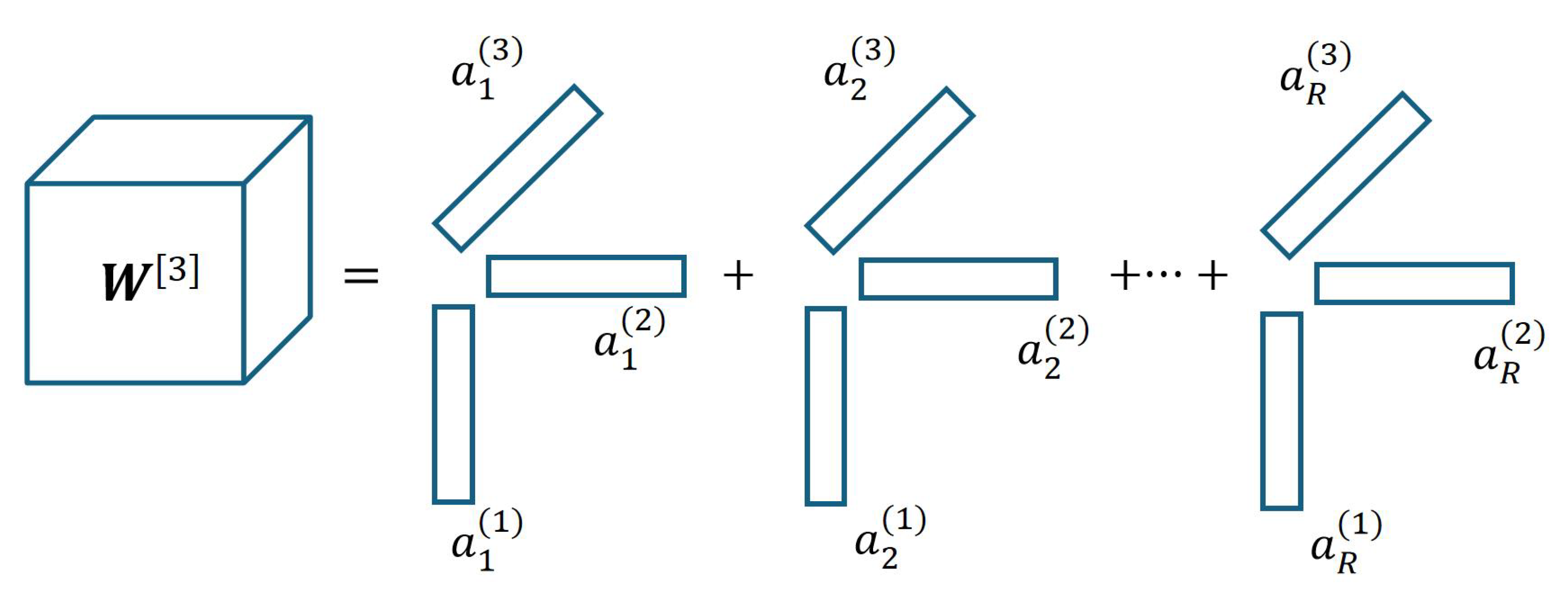
where R is decomposition rank, and n is the order of the decomposed tensor . Here, we use COMP/PARAFAC (CP) decomposition to execute this process. CP decomposition has been widely adopted for modeling multilinear relationships in machine learning applications [31,51]. In contrast to Tucker decomposition, CP decomposition provides both computational and structural advantages for our neuronal formula discovery framework. Computationally, CP decomposition requires only parameters for an n-th order tensor of size , compared to Tucker’s complexity, enabling efficient handling of high-order polynomial terms. An example of CP decomposition is illustrated in Figure 4. While other tensor decomposition approaches could be explored (e.g., tensor ring decomposition, hierarchical Tucker decomposition) [52,53], the efficiency and structural benefits of CP decomposition have already aligned well with the requirements of our polynomial modeling framework.
Figure 3.
A rank-R CP decomposition of a third-order tensor.
Moreover, the incorporation of the trigonometric term serves a pivotal purpose. It extends the model’s capacity to capture periodic patterns and high-frequency components that intrinsically appear in many real-world datasets [54]. This is particularly crucial as pure polynomial expansions exhibit limited spectral sensitivity.
We then impose sparsity constraints through regularization on both the coefficients and weight tensors to promote computational efficiency. Specifically, since each tensor is decomposed using CP decomposition as , we apply sparsity regularization directly to the factor matrices. Thus, the complete optimization objective becomes
where is the task-specific loss function, set to mean squared error (MSE) for regression and cross-entropy (CE) loss for classification. This structured sparsity approach encourages the discovery of interpretable and simplified polynomial formulas while maintaining computational efficiency through the low-rank tensor representation.
To further enhance the compactness of the discovered neuronal formula beyond the regularization’s sparsity induction, we introduce a post-training thresholding mechanism for explicit term selection. While the regularization effectively drives many coefficients toward zero, empirical observations reveal that a non-negligible portion of coefficients retain small but non-zero values, which cumulatively increase model complexity without substantial predictive contribution. The thresholding mechanism is a statistically grounded pruning strategy: After model convergence, we compute the mean and the standard deviation of the absolute values of all coefficients , then construct the final neuronal formula by retaining only terms whose coefficients satisfy , where . This can further increase the stability of identified formulas.
Remark 1. Three key features of the proposed method warrant emphasis. i) The higher-order polynomial architecture systematically enables the learning of the polynomials. It is noticed that Eq. (2) is rather inclusive, e.g., it identifies multi-order variable interactions. This structural flexibility facilitates sophisticated nonlinear approximations, aligning the model more closely with the underlying data distribution. ii) The integration of trainable coefficients with the regularization imposes selective sparsity constraints on the polynomial expansion. Specifically, the regularization term induces sparsity by driving coefficients of less predictive terms toward zero, thereby automatically pruning nonessential higher-order components and yielding a parsimonious architecture. iii) The complementary regularization on the coefficients enforces structured sparsity in the parameter space. This dual regularization strategy enhances feature selection while simultaneously improving computational efficiency—a critical advantage in high-dimensional contexts. Collectively, these design choices balance expressive capacity with compactness, ensuring robust performance without overparameterization.
3.2.2. Task-Driven Network Construction
In the second stage, the discovered neuronal formula is first parameterized into neuron-like structures. The selected polynomial and trigonometric terms are assigned trainable weights and integrated into neural network architectures. For tabular data processing, we employ fully connected neural networks. A polynomial with the maximum polynomial order of 3 is expressed as
with being the ReLU activation function. If a specific order term is absent in the neuronal formula, its corresponding weight and bias parameters are initialized to zero.
Moreover, we extend our framework to convolutional neurons for images. As mentioned, the trigonometric term is incorporated to model periodic patterns and high-frequency components inherent in high-dimensional images. Consequently, the complete neuronal formula is structured as follows:
where * denotes the convolution operation.
Finally, we introduce a simple initialization strategy to enhance training stability. Followed by [33], the weight matrix is initialized as , where , while all other weights are initialized to a tiny number such as 0.001. This strategy ensures that the network initially behaves like linear neurons and gradually learns higher-order terms during training. This strategy has been demonstrated the effectiveness in training quadratic neurons [55].
4. Super-Expressive Property Theory of Task-Driven Neuron
In this section, we formally prove that task-driven neurons that modify the aggregation function can also achieve the super-expressive property. Our theory is established based on the chaotic theory. Mathematically, we have the following theorem:
Theorem 1.
Let be a continuous function. Then, for any , there exists a function h generated by a task-driven network with a fixed number of parameters, such that
Proof sketch: Our proof leverages heavily the framework of [18] that turns via the interval partition the function approximation into the point-fitting problem. Hence, for consistency and readability, we inherit their notations and framework. The proof idea is divided into three steps:
Step 1. As Figure 4 shows, in equal distance, divide into small intervals for , where K is the number of intervals. The left endpoint of is . A higher K leads to a smaller approximation error. We construct a piecewise constant function h to approximate f. The error can be arbitrarily small as long as the divided interval goes tiny. Based on the interval division, we have
where is a point from .
Step 2. As Figure 4 shows, use the function mapping all x in the interval to k, where is the flooring function. There exists a one-to-one correspondence between k and . Thus, via dividing intervals and applying the floor function, the problem of approximation is simplified into a point-fitting problem. Therefore, we just need to construct a point-fitting function to map k to .
Step 3. In [18], the point-fitting function is constructed as based on Proposition 1. In contrast, we solve it with a discrete dynamic system that is constructed by a network made of task-driven neurons. We design a sub-network to generate a function mapping k approximately to for each k. Then for any and , which implies on . is based on Lemma 1, where T is a unimodal function from that can also induce the dense trajectory.
Proposition 1
where .
Definition 1
([57]). A map is said to be unimodal if there exists a turning point such that the map f can be expressed as
where and are continuous, differentiable except possibly at finite points, monotonically increasing and decreasing, respectively, and onto the unit-interval in the sense that and .
Lemma 1
(Dense Trajectory). There exists a measure-preserving transformation T, generated from a network with task-driven neurons, such that there exists ξ with dense in . In other words, for any x and , there exist ξ and the corresponding composition times m, such that
Particularly, we refer to ξ as a transitive point.
Proof.
Since we extensively apply polynomials to prototyping task-driven neurons, we prove that a polynomial of any order can fulfill the condition. The proof can be easily extended to other functions with minor twists.
i) Given a polynomial of any order, as shown in Figure 5, through cutting, translation, flipping, and scaling, we can construct a unimodal map .
ii) For a unimodal map T, we can show that for any two non-empty sets with , there exists an m such that . As Figure 6 shows, this is because a set U with will always contain a tiny subset such that . Then, naturally due to .
iii) The above property can lead to a dense orbit, combining that is with a countable basis, according to Proposition 2 of [58]. For the sake of self-sufficiency, we include their proof here.
Let be a countable base for X. For , the set is open by continuity of f. This set is also dense in X. To see this let U be any non-empty open set. Because of topological transitivity there exists a with . This gives and . Thus is dense. By the Baire category theorem, the set is dense in X. Now, the orbit of any point is dense in X.
Because, given any non-empty open , there is an with and with . This means . Thus the orbit of enters any U.
□
Proof of Theorem 1. Now, we are ready to prove Theorem 1. First, the input x is mapped into an integer k, whereas k corresponds to the composition time . Next, a network module representing T is copied times and composed times such that . Since can approximate well, also approximates well.
Theorem 1 can be easily generalized into multivariate functions by using the Kolmogorov-Arnold theorem.
Proposition 2.
For any , there exist continuous functions for and such that any continuous function can be represented as
where is a continuous function for each .
Remark 2. Our construction saves the parametric complexity. In [18], though the number of parameters remains unchanged, the values of parameters increase as long as n increases. Therefore, the entire parametric complexity goes up. In contrast, in our construction, the parameter value of T is also fixed for different . Yet, T is copied and composed times. The overall parametric complexity remains unchanged. What increases herein is computational complexity. Therefore, we call for brevity our construction “super-super-expressive”.
5. Comparative Experiments on NeuronSeek
This section presents a comprehensive experimental evaluation of our proposed method and the previous NeuronSeek-SR [12]. First, we systematically demonstrate the superior performance and enhanced stability of NeuronSeek-TD compared to the previous NeuronSeek-SR. The results demonstrate that pursuing stability in NeuronSeek-TD does not hurt the representation power of the resultant task-driven neurons and even present better results.
5.1. Experiment on Synthetic Data
Here, we adopt the synthetic data to compare the performance of NeuronSeek-TD and NeuronSeek-SR. The synthetic data are generated by adding noise perturbations to the known ground-truth functions. We then measure the regression error (MSE) of the formulas of NeuronSeek-SR and NeuronSeek-TD on the synthetic data.
5.1.1. Experimental Settings
Eight multivariate polynomials are constructed as shown in Table 2. For simplicity and conciseness, we prescribe:
where denotes a constant vector, represents the input vector, and ⊙ denotes the Hadamard product. The elements of are uniformly sampled from the interval . We set to simulate multi-dimensional inputs.
To evaluate the noise robustness of the proposed methods, we introduce three noise levels through
where y denotes the noise-free polynomial output, is the noisy observation, is a standard normal random vector, controls the relative noise level, and represents the root mean square (RMS) of the data:
Here, specifies the number of data points. For NeuronSeek-SR, we configure a population size of 1,000 with the maximum of 50 generations. NeuronSeek-TD is optimized using Adam for 50 epochs. The noise levels are set to respectively. We quantify the regression performance using the mean squared error (MSE) of the discovered neuronal formulae. Lower MSE values indicate better preservation of the underlying data characteristics.
5.1.2. Experimental Results
The performance comparison on the synthetic data is presented in Table 2. Our proposed NeuronSeek-TD demonstrates consistent superiority over NeuronSeek-SR across all generated data, with particularly notable improvements on the data derived from the function . This performance advantage remains robust under varying noise levels.
To assess computational efficiency, we measure the average execution time for both methods. NeuronSeek-TD achieves substantial computational savings, requiring less than half the execution time of the SR-based approach while maintaining comparable solution quality. These results collectively demonstrate that our method achieves both superior accuracy and greater computational efficiency.
5.2. Experiments on Uniqueness and Stability
Here, we demonstrate that NeuronSeek-SR exhibits instability in terms of resulting in divergent formulas under minor perturbations in initialization, while NeuronSeek-TD maintains good consistency.
5.2.1. Experimental Settings
Our experimental protocol consists of two benchmark datasets: the phoneme dataset (a classification task classifying nasal and oral sounds) and the airfoil self-noise dataset (a regression task modeling self-generated noise of airfoil). These public datasets are chosen from the OpenML website to represent both classification and regression tasks, ensuring a comprehensive evaluation across different problem types. For each dataset, we introduce four levels of Gaussian noise () to simulate real-world perturbations. We train 10 independent instances of each method under identical initialization. For comparison, NeuronSeek-SR based on GP uses a population of 3,000 candidates evolved over 20 generations, whereas NeuronSeek-TD methods—employing CP decomposition and Tucker decomposition—rely on a model optimized via Adam over 20 epochs.
To quantify the uniqueness of SR and TD methods, we track two diversity metrics:
- Epoch-wise diversity represents the number of different formulas within each epoch (or generation) across all initializations. For instance, and are considered identical, whereas and are distinct.
- Cumulative diversity measures the average number of unique formulas identified per initialization as the optimization goes on.
5.2.2. Experimental Results
The results of phoneme and airfoil self-noise datasets are depicted in Figure 8 and Figure 7, respectively. From the epoch-wise diversity (Figure 8 (a) and Figure 7 (a)), we have several important observations: Firstly, GP-based SR demonstrates a rapid increase in the number of discovered formulas within each epoch. After training, it produces more unique formulas compared to TD-based methods (CP and Tucker). This indicates that SR is sensitive to initialization conditions. Secondly, as noise levels increase, the GP method discovers nearly 10 distinct formulas across 10 initializations. With higher noise, every initialization produces a completely different formula structure. These behaviors highlight the instability of GP-based SR when dealing with noisy data, as minor perturbations in initialization or data noise can lead to substantially different symbolic expressions.
Furthermore, regarding cumulative diversity (Figure 8(b) and Figure 7(b)), we can observe that GP-based SR constantly discovers an increasing number of different formulas, while TD methods tend to stabilize during training. This indicates that the GP algorithm struggles to converge to a consistent symbolic formula. In contrast, the asymptotic behavior exhibited by TD-based methods demonstrates their superior stability and convergence properties when identifying symbolic expressions. Moreover, the CP-based method suggests the best resilience against initialization variability.
5.3. Superiority of NeuronSeek-TD over NeuronSeek-SR
To validate the superior performance of NeuronSeek-TD over NeuronSeek-SR, we conduct experiments across 16 benchmark datasets—8 for regression and 8 for classification—selected from scikit-learn and OpenML repositories. First, we use NeuronSeek-TD and NeuronSeek-SR simultaneously to search for the optimal formula. Second, we construct fully connected networks (FCNs) with neurons taking these discovered formulas as their aggregation functions. To verify the ability of NeuronSeek-TD, the structures of neural networks are carefully set, such that NeuronSeek-TD has equal or fewer parameters than NeuronSeek-SR.
Comprehensive implementation details and test results are provided in Table 3. For regression tasks, the dataset is partitioned into training and test sets in an 8:2 ratio. The activation function is with MSE as the loss function and as the optimizer. For classification tasks, the same train-test split is applied, using the activation function. The loss function and optimizer are set to CE and , respectively. All experiments are repeated 10 times and reported by mean and standard deviation, with MSE for regression and accuracy for classification.
The regression results in Table 3 demonstrate that NeuronSeek-SR exhibits larger fitting errors compared to NeuronSeek-TD, along with higher standard deviations in MSE values. A notable example is the airfoil self-noise dataset, where NeuronSeek-TD outperforms NeuronSeek-SR by a significant margin, achieving a 9% reduction in MSE. Furthermore, NeuronSeek-TD shows superior performance on both the California housing and abalone datasets while utilizing fewer parameters. These results collectively indicate that NeuronSeek-TD possesses stronger regression capabilities than NeuronSeek-SR.
This performance advantage extends to classification tasks, where NeuronSeek-TD consistently achieves higher accuracy than NeuronSeek-SR. Particularly in the HELOC and orange-vs-grapefruit datasets, NeuronSeek-TD attains better classification performance with greater parameter efficiency. The observed improvements across both regression and classification tasks suggest that NeuronSeek-TD offers superior modeling capabilities compared to NeuronSeek-SR.
5.4. Comparison of Tensor Decomposition Methods
Our framework employs the CP decomposition for neuronal discovery. To empirically validate this choice, we conduct a comparative analysis of some tensor decomposition methods used in NeuronSeek-TD.
5.4.1. Experimental Settings
Generally, we follow the previous experimental settings in Section 5.3: 16 tabular datasets and the same network structures as described in Table 3. We adopt CP decomposition and Tucker decomposition respectively for tensor processing in NeuronSeek-TD. We employ MSE for regression tasks, while classification accuracy is utilized for classification tasks.
5.4.2. Experimental results
First, Figure 9 illustrates that, for most datasets, the two decomposition methods exhibit comparable performance. Exceptions include airfoil Self-Noise and electricity datasets, where the two methods show slight performance differences. This observation suggests that variations in TD methods do not substantially impact the final results. Second, as shown in Figure 10, the CP-based method achieves a 42% reduction in computational time. This result verifies that the CP method offers a computational advantage over the Tucker method.
6. Competitive Experiments of NeuronSeek-TD over Other Baselines
6.1. Experiment on Tabular Data
To further illustrate the superiority of NeuronSeek-TD, we compare it with other state-of-the-art models over 4 real-world tabular tasks: Electron Collision Prediction1, Asteroid Prediction2, Heart Failure Detection3, and Stellar Classification4). We adopt 7 advanced machine learning methods, namely XGBoost [59], LightGBM [60], CatBoost [61], TabNet [62], TabTransformer [63], FT-Transformer [64], DANETs [65] and NeuronSeek-SR [12] as the baselines to compare with NeuronSeek-TD. Moreover, our proposed model and NeuronSeek-SR replace standard neurons with what are discovered by NeuronSeek-TD and NeuronSeek-SR, respectively.
All datasets are randomly split into training, validation, and test sets in a 0.8:0.1:0.1 ratio. For regression tasks (electron collision and asteroid prediction), we use the MSE as an evaluation metric, while for classification tasks with imbalanced labels (heart failure detection and stellar classification), we adopt the F1 score. Detailed experiment information is shown in Table 4.
Results are compared in Table 5. It can be seen that TabTransformer demonstrates competitive performance on the particle collision dataset. However, its effectiveness sharply declines on the asteroid prediction. In contrast, CatBoost and TabNet exhibit more consistent yet suboptimal results across four datasets. Lastly, the proposed NeuronSeek-TD method is the best performer, achieving the lowest error rates and highest F1 scores uniformly across all four benchmarks. Notably, NeuronSeek-TD significantly outperforms FT-Transformer and DANET. This significant margin underscores the efficacy of its task-adaptive architecture in recognizing feature interactions without domain-specific tuning.
6.2. Experiments on Images
To evaluate the performance enhancement of NeuronSeek-TD in computer vision tasks, we integrate it into several established convolutional neural network architectures: ResNet [3], DenseNet [66], SeResNet [67], and GoogLeNet [68]. Notably, we replace the first convolutional layer of each network block with a TN convolutional layer employing the discovered formula . It should be noted that the original NeuronSeek-SR was not designed for high-dimensional image tasks due to convergence difficulties. Our implementation focuses on NeuronSeek-TD and follows the standardized training protocol from a popular image classification repository5, incorporating several advanced training techniques: Learning rate scheduling via and , regularization through , and optimization using . We use grid search to fine-tune the learning rate from 0.5 to 0.05. All models are trained for 200 epochs with a batch size of 128. We evaluate the results using classification accuracy averaged over 10 independent runs.
We adopt four standard image datasets to validate the model: CIFAR 10/100 [69], SVHN [70], and STL10 [71]. The training and validation sets are split with a ratio of 0.9 : 0.1. In particular, images from the STL10 dataset are resized to to fit the input of the model. The classification results are summarized in Table 6.
Our experiments demonstrate that task-driven neuronal layers consistently enhance the baseline performance across multiple datasets. Notably, NeuronSeek-augmented ResNet18 achieves a 2% accuracy improvement on both CIFAR 100 and STL10 datasets. While SeResNet exhibits median performance on CIFAR and SVHN datasets, its performance degrades on STL10; however, TN layers compensate for this degradation by boosting its accuracy by 10%. These results suggest that task-driven neuronal formula discovery can effectively unlock the latent potential of fundamental network architectures.
7. Discussions and Conclusions
In this paper, we have proposed a novel method in the framework of NeuronSeek to enhance the capabilities of a neural network. Compared to neural architecture search (NAS) [72], NeuronSeek provides a different approach. Rather than modifying the overall model structure, NeuronSeek optimizes solely at the neuronal level by searching for optimal aggregation formulas. Firstly, we have introduced tensor decomposition to prototype stable task-driven neurons. Secondly, we have provided theoretical guarantees demonstrating that these neurons can maintain the super-super-expressive property. At last, through extensive empirical evaluation, we show that our proposed framework consistently outperforms baseline models while achieving the state-of-the-art results across diverse datasets and tasks. These advancements establish task-driven neurons as an effective addition in the design of task-specific neural network components, offering both theoretical soundness and practical efficacy.
References
- Yang, X.; Song, Z.; King, I.; Xu, Z. A Survey on Deep Semi-Supervised Learning. IEEE Transactions on Knowledge and Data Engineering 2023, 35, 8934–8954. [CrossRef]
- Wang, S.; Cao, J.; Yu, P.S. Deep Learning for Spatio-Temporal Data Mining: A Survey. IEEE Transactions on Knowledge and Data Engineering 2022, 34, 3681–3700. [CrossRef]
- He, K.; Zhang, X.; Ren, S.; Sun, J. Deep residual learning for image recognition. In Proceedings of the Proceedings of the IEEE Conference on Computer Vision and Pattern Recognition (CVPR), 2016, pp. 770–778.
- Vaswani, A.; Shazeer, N.; Parmar, N.; Uszkoreit, J.; Jones, L.; Gomez, A.N.; Kaiser, Ł.; Polosukhin, I. Attention is all you need. In Proceedings of the Advances in Neural Information Processing Systems (NeurIPS), 2017, pp. 5998–6008.
- MacAvaney, S.; Soldaini, L.; Yates, A. Mamba: Learning neural IR models with random walks. In Proceedings of the Proceedings of the 44th International ACM SIGIR Conference on Research and Development in Information Retrieval (SIGIR), 2021, pp. 1642–1646.
- Zador, A.; Escola, S.; Richards, B.; et al.. Catalyzing next-generation Artificial Intelligence through NeuroAI. Nature Communications 2023, 14, 1597. [CrossRef]
- Fan, F.L.; Li, Y.; Zeng, T.; Wang, F.; Peng, H. Towards NeuroAI: introducing neuronal diversity into artificial neural networks. Med-X 2025, 3, 2.
- Peng, H.; Xie, P.; Liu, L.; et al.. Morphological diversity of single neurons in molecularly defined cell types. Nature 2021, 598, 174–181. [CrossRef]
- Xu, Z.; Yu, F.; Xiong, J.; Chen, X. Quadralib: A Performant Quadratic Neural Network Library for Architecture Optimization and Design Exploration. In Proceedings of the Proceedings of Machine Learning and Systems, 2022, Vol. 4, pp. 503–514.
- Chrysos, G.G.; Moschoglou, S.; Bouritsas, G.; Deng, J.; Panagakis, Y.; Zafeiriou, S. Deep Polynomial Neural Networks. IEEE Transactions on Pattern Analysis and Machine Intelligence 2020.
- Xu, W.; Song, Y.; Gupta, S.; Jia, D.; Tang, J.; Lei, Z.; Gao, S. Dmixnet: a dendritic multi-layered perceptron architecture for image recognition. Artificial Intelligence Review 2025, 58, 129.
- Fan, F.L.; Wang, M.; Dong, H.; Ma, J.; Zeng, T. No One-Size-Fits-All Neurons: Task-based Neurons for Artificial Neural Networks. arXiv preprint 2024.
- Schmidt, M.; Lipson, H. Distilling free-form natural laws from experimental data. Science 2009, 324, 81–85.
- Bartlett, D.J.; Desmond, H.; Ferreira, P.G. Exhaustive Symbolic Regression. IEEE Transactions on Evolutionary Computation 2023.
- Espejo, P.G.; Ventura, S.; Herrera, F. A survey on the application of genetic programming to classification. IEEE Transactions on Systems, Man, and Cybernetics, Part C (Applications and Reviews) 2009, 40, 121–144.
- de Carvalho, M.G.; Laender, A.H.F.; Goncalves, M.A.; da Silva, A.S. A Genetic Programming Approach to Record Deduplication. IEEE Transactions on Knowledge and Data Engineering 2012, 24, 399–412. [CrossRef]
- Yarotsky, D. Elementary superexpressive activations. In Proceedings of the International Conference on Machine Learning. PMLR, 2021, pp. 11932–11940.
- Shen, Z.; Yang, H.; Zhang, S. Deep Network Approximation: Achieving Arbitrary Accuracy with Fixed Number of Neurons. Journal of Machine Learning Research 2022, 23, 1–60.
- Shen, Z.; Yang, H.; Zhang, S. Neural network approximation: Three hidden layers are enough. Neural Networks 2021, 141, 160–173. [CrossRef]
- Makke, N.; Chawla, S. Interpretable Scientific Discovery with Symbolic Regression: A Review. arXiv preprint arXiv:2211.10873 2023.
- Kolda, T.G.; Bader, B.W. Tensor decompositions and applications. SIAM Review 2009, 51, 455–500.
- Fukushima, K. Recent advances in the deep CNN neocognitron. Nonlinear Theory and Its Applications, IEICE 2019, 10, 304–321. [CrossRef]
- Zhang, Z.; Ding, X.; Liang, X.; Zhou, Y.; Qin, B.; Liu, T. Brain and Cognitive Science Inspired Deep Learning: A Comprehensive Survey. IEEE Transactions on Knowledge and Data Engineering 2025, 37, 1650–1671. [CrossRef]
- Plant, C.; Zherdin, A.; Sorg, C.; Meyer-Baese, A.; Wohlschläger, A.M. Mining Interaction Patterns among Brain Regions by Clustering. IEEE Transactions on Knowledge and Data Engineering 2014, 26, 2237–2249. [CrossRef]
- Zoumpourlis, G.; Doumanoglou, A.; Vretos, N.; Daras, P. Non-linear convolution filters for CNN-based learning. In Proceedings of the Proceedings of the IEEE International Conference on Computer Vision (ICCV), 2017, pp. 4761–4769.
- Jiang, Y.; Yang, F.; Zhu, H.; Zhou, D.; Zeng, X. Nonlinear CNN: Improving CNNs with Quadratic Convolutions. Neural Computing and Applications 2020, 32, 8507–8516.
- Mantini, P.; Shah, S.K. CQNN: Convolutional Quadratic Neural Networks. In Proceedings of the 2020 25th International Conference on Pattern Recognition (ICPR), 2021, pp. 9819–9826. [CrossRef]
- Goyal, M.; Goyal, R.; Lall, B. Improved Polynomial Neural Networks with Normalised Activations. In Proceedings of the 2020 International Joint Conference on Neural Networks (IJCNN). IEEE, 2020, pp. 1–8.
- Bu, J.; Karpaten, A. Quadratic Residual Networks: A New Class of Neural Networks for Solving Forward and Inverse Problems in Physics Involving PDEs. In Proceedings of the Proceedings of the 2021 SIAM International Conference on Data Mining (SDM). SIAM, 2021, pp. 675–683.
- Fan, F.; Cong, W.; Wang, G. A New Type of Neurons for Machine Learning. International Journal for Numerical Methods in Biomedical Engineering 2018, 34, e2920.
- Chrysos, G.; Moschoglou, S.; Bouritsas, G.; Deng, J.; Panagakis, Y.; Zafeiriou, S.P. Deep Polynomial Neural Networks. IEEE Transactions on Pattern Analysis and Machine Intelligence 2021.
- Chrysos, G.G.; Georgopoulos, M.; Deng, J.; Kossaifi, J.; Panagakis, Y.; Anandkumar, A. Augmenting Deep Classifiers with Polynomial Neural Networks. In Proceedings of the European Conference on Computer Vision. Springer, 2022, pp. 692–716.
- Chrysos, G.G.; Wang, B.; Deng, J.; Cevher, V. Regularization of polynomial networks for image recognition. In Proceedings of the Proceedings of the IEEE/CVF Conference on Computer Vision and Pattern Recognition, 2023, pp. 16123–16132.
- Kiyani, E.; Shukla, K.; Karniadakis, G.E.; Karttunen, M. A framework based on symbolic regression coupled with extended physics-informed neural networks for gray-box learning of equations of motion from data. Computer Methods in Applied Mechanics and Engineering 2023, 415, 116258.
- Wang, R.; Sun, D.; Wong, R.K. Symbolic Minimization on Relational Data. IEEE Transactions on Knowledge and Data Engineering 2023, 35, 9307–9318. Note: Publication year (2023) differs from DOI year (2022), . [CrossRef]
- Sahoo, S.; Lampert, C.; Martius, G. Learning Equations for Extrapolation and Control. In Proceedings of the Proceedings of the 35th International Conference on Machine Learning. PMLR, 2018, Vol. 80, PMLR, pp. 4442–4450.
- Tohme, T.; Khojasteh, M.J.; Sadr, M.; Meyer, F.; Youcef-Toumi, K. ISR: Invertible Symbolic Regression. arXiv preprint 2024, arXiv:2405.06848. Submitted on 10 May 2024, . [CrossRef]
- Liu, Z.; Wang, Y.; Vaidya, S.; Ruehle, F.; Halverson, J.; Soljačić, M.; Hou, T.Y.; Tegmark, M. Kan: Kolmogorov-arnold networks. arXiv preprint arXiv:2404.19756 2024.
- Li, C.; Liu, X.; Li, W.; Wang, C.; Liu, H.; Liu, Y.; Chen, Z.; Yuan, Y. U-kan makes strong backbone for medical image segmentation and generation. In Proceedings of the Proceedings of the AAAI Conference on Artificial Intelligence, 2025, Vol. 39, pp. 4652–4660.
- Toscano, J.D.; Oommen, V.; Varghese, A.J.; Zou, Z.; Ahmadi Daryakenari, N.; Wu, C.; Karniadakis, G.E. From pinns to pikans: Recent advances in physics-informed machine learning. Machine Learning for Computational Science and Engineering 2025, 1, 1–43.
- Kamienny, P.a.; d’Ascoli, S.; Lample, G.; Charton, F. End-to-end Symbolic Regression with Transformers. In Proceedings of the Advances in Neural Information Processing Systems; Koyejo, S.; Mohamed, S.; Agarwal, A.; Belgrave, D.; Cho, K.; Oh, A., Eds. Curran Associates, Inc., 2022, Vol. 35, pp. 10269–10281.
- Kim, S.; et al. Integration of neural network-based symbolic regression in deep learning for scientific discovery. IEEE Transactions on Neural Networks and Learning Systems 2020, 32, 4166–4177.
- Valipour, M.; You, B.; Panju, M.H.; Ghodsi, A. SymbolicGPT: A Generative Transformer Model for Symbolic Regression. In Proceedings of the Second Workshop on Efficient Natural Language and Speech Processing (ENLSP-II), NeurIPS, 2022.
- Newell, A.; Simon, H. The logic theory machine–A complex information processing system. IRE Transactions on information theory 1956, 2, 61–79.
- Taha, I.A.; Ghosh, J. Symbolic Interpretation of Artificial Neural Networks. IEEE Transactions on Knowledge and Data Engineering 1999, 11, 448–463. [CrossRef]
- Smolensky, P. Connectionist AI, symbolic AI, and the brain. Artificial Intelligence Review 1987, 1, 95–109.
- Foggia, P.; Genna, R.; Vento, M. Symbolic vs. Connectionist Learning: An Experimental Comparison in a Structured Domain. IEEE Transactions on Knowledge and Data Engineering 2001, 13, 176–195. [CrossRef]
- Fu, L. Knowledge Discovery by Inductive Neural Networks. IEEE Transactions on Knowledge and Data Engineering 1999, 11, 992–998. [CrossRef]
- Maiorov, V.; Pinkus, A. Lower bounds for approximation by MLP neural networks. Neurocomputing 1999, 25, 81–91. [CrossRef]
- Zhang, S.; Lu, J.; Zhao, H. On Enhancing Expressive Power via Compositions of Single Fixed-Size ReLU Network. In Proceedings of the Proceedings of the 40th International Conference on Machine Learning; Krause, A.; Brunskill, E.; Cho, K.; Engelhardt, B.; Sabato, S.; Scarlett, J., Eds. PMLR, 23–29 Jul 2023, Vol. 202, Proceedings of Machine Learning Research, pp. 41452–41487.
- Guo, W.; Kotsia, I.; Patras, I. Tensor Learning for Regression. IEEE Transactions on Image Processing 2012.
- Yuan, L.; Li, C.; Cao, J.; Zhao, Q. Randomized Tensor Ring Decomposition and Its Application to Large-scale Data Reconstruction. In Proceedings of the ICASSP 2019 - 2019 IEEE International Conference on Acoustics, Speech and Signal Processing (ICASSP), 2019, pp. 2127–2131. [CrossRef]
- Grasedyck, L. Hierarchical Singular Value Decomposition of Tensors. SIAM Journal on Matrix Analysis and Applications 2010, 31, 2029–2054, [. [CrossRef]
- Tancik, M.; Srinivasan, P.; Mildenhall, B.; Fridovich-Keil, S.; Raghavan, N.; Singhal, U.; Ramamoorthi, R.; Barron, J.; Ng, R. Fourier Features Let Networks Learn High Frequency Functions in Low Dimensional Domains. In Proceedings of the Advances in Neural Information Processing Systems, 2020, Vol. 33.
- Fan, F.L.; Li, M.; Wang, F.; Lai, R.; Wang, G. On expressivity and trainability of quadratic networks. IEEE Transactions on Neural Networks and Learning Systems 2023.
- Katok, A.; Katok, A.; Hasselblatt, B. Introduction to the modern theory of dynamical systems; Cambridge university press, 1995.
- Huang, W. On complete chaotic maps with tent-map-like structures. Chaos, Solitons & Fractals 2005, 24, 287–299. [CrossRef]
- Değirmenci, N.; Koçak, Ş. Existence of a dense orbit and topological transitivity: when are they equivalent? Acta Mathematica Hungarica 2003, 99, 185–187.
- Chen, T.; Guestrin, C. XGBoost: A Scalable Tree Boosting System. In Proceedings of the Proceedings of the 22nd ACM SIGKDD International Conference on Knowledge Discovery and Data Mining (KDD), 2016, pp. 785–794.
- Ke, G.; Meng, Q.; Finley, T.; Wang, T.; Chen, W.; Ma, W.; Ye, Q.; Liu, T.Y. LightGBM: A Highly Efficient Gradient Boosting Decision Tree. In Proceedings of the Advances in Neural Information Processing Systems (NeurIPS), 2017, Vol. 30, pp. 1–9.
- Hancock, J.T.; Khoshgoftaar, T.M. CatBoost for Big Data: An Interdisciplinary Review. Journal of Big Data 2020, 7, 1–45.
- Arik, S.Ö.; Pfister, T. TabNet: Attentive Interpretable Tabular Learning. In Proceedings of the Proceedings of the AAAI Conference on Artificial Intelligence (AAAI), 2021, Vol. 35, pp. 6679–6687.
- Huang, X.; Khetan, A.; Cvitkovic, M.; Karnin, Z. TabTransformer: Tabular Data Modeling Using Contextual Embeddings. arXiv preprint arXiv:2012.06678 2020.
- Gorishniy, Y.; Rubachev, I.; Khrulkov, V.; Babenko, A. Revisiting Deep Learning Models for Tabular Data. In Proceedings of the Advances in Neural Information Processing Systems (NeurIPS), 2021, Vol. 34, pp. 18932–18943.
- Chen, J.; Liao, K.; Wan, Y.; Chen, D.Z.; Wu, J. DANets: Deep Abstract Networks for Tabular Data Classification and Regression. In Proceedings of the Proceedings of the AAAI Conference on Artificial Intelligence (AAAI), 2022, Vol. 36, pp. 3930–3938.
- Huang, G.; Liu, Z.; Van Der Maaten, L.; Weinberger, K.Q. Densely connected convolutional networks. In Proceedings of the Proceedings of the IEEE conference on computer vision and pattern recognition, 2017, pp. 4700–4708.
- Hu, J.; Shen, L.; Sun, G. Squeeze-and-excitation networks. In Proceedings of the Proceedings of the IEEE conference on computer vision and pattern recognition, 2018, pp. 7132–7141.
- Szegedy, C.; Liu, W.; Jia, Y.; Sermanet, P.; Reed, S.; Anguelov, D.; Erhan, D.; Vanhoucke, V.; Rabinovich, A. Going deeper with convolutions. In Proceedings of the Proceedings of the IEEE conference on computer vision and pattern recognition, 2015, pp. 1–9.
- Krizhevsky, A.; Hinton, G.; et al. Learning multiple layers of features from tiny images 2009.
- Netzer, Y.; Wang, T.; Coates, A.; Bissacco, A.; Wu, B.; Ng, A.Y.; et al. Reading digits in natural images with unsupervised feature learning. In Proceedings of the NIPS workshop on deep learning and unsupervised feature learning. Granada, 2011, Vol. 2011, p. 4.
- Coates, A.; Ng, A.; Lee, H. An analysis of single-layer networks in unsupervised feature learning. In Proceedings of the Proceedings of the fourteenth international conference on artificial intelligence and statistics. JMLR Workshop and Conference Proceedings, 2011, pp. 215–223.
- White, C.; Safari, M.; Sukthanker, R.; Ru, B.; Elsken, T.; Zela, A.; Dey, D.; Hutter, F. Neural architecture search: Insights from 1000 papers. arXiv preprint arXiv:2301.08727 2023.
| 1 | |
| 2 | |
| 3 | |
| 4 | |
| 5 |
Figure 1.
Task-driven neuron based on the vectorized symbolic regression (NeuronSeek-SR).
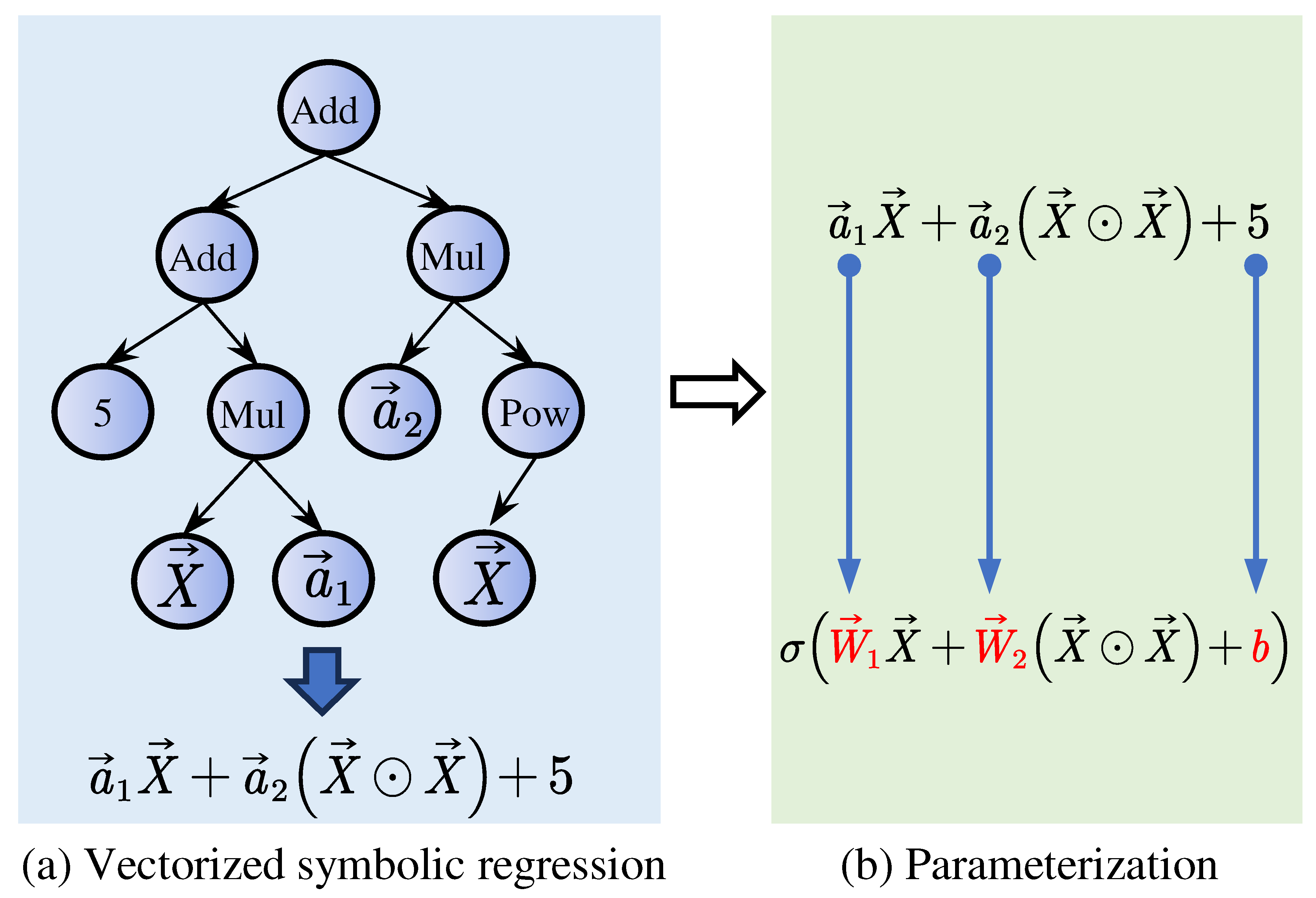
Figure 2.
The overall framework of the proposed method. In the first stage, the input data, regardless of tables and images, are flattened into a vector representation and processed using an initial formula for neuronal search. A stable formula is then generated through CP decomposition. In the second stage, the neuronal formula is parameterized and integrated into various neural network backbones for task-specific applications.
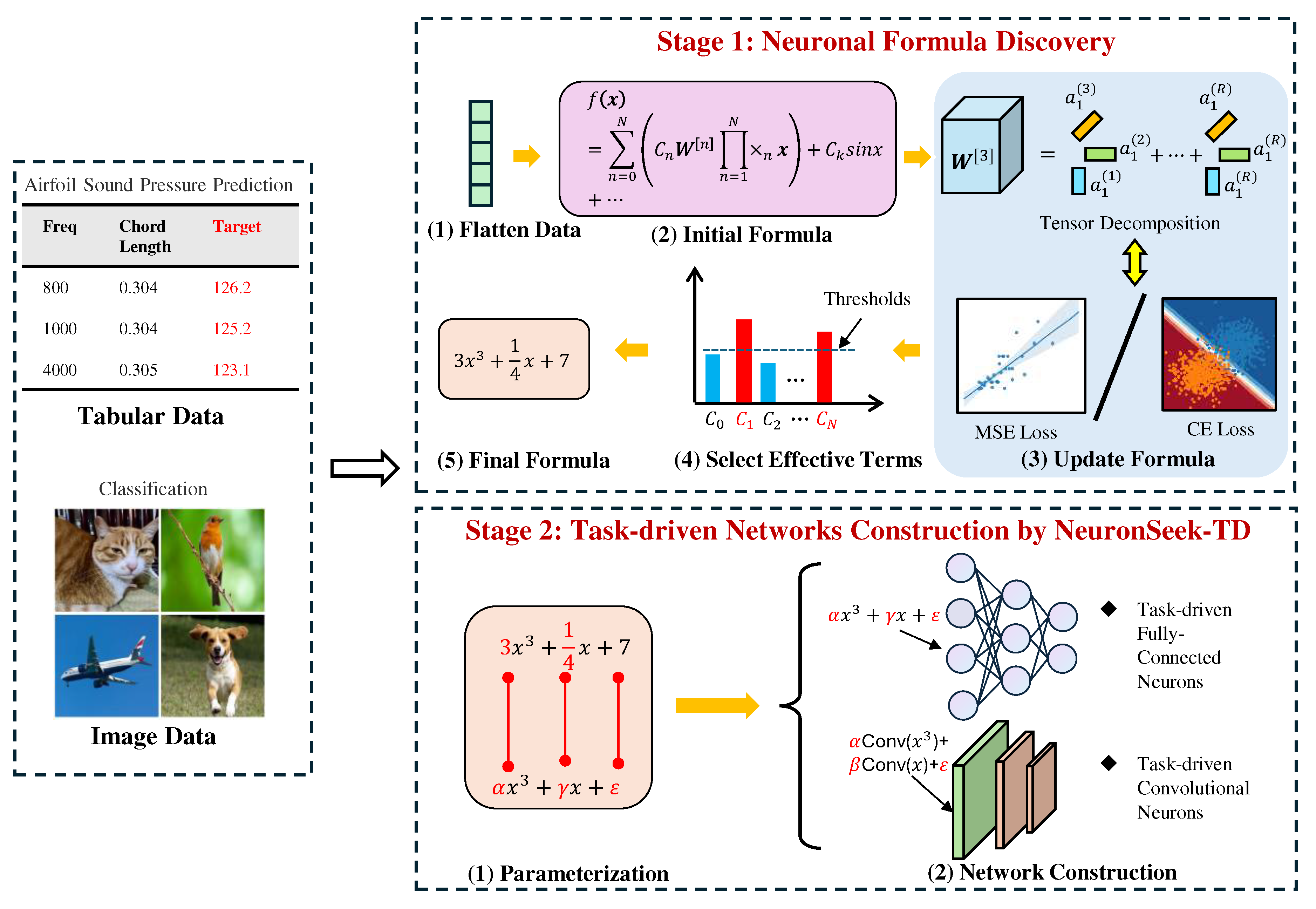
Figure 4.
A sketch of our proof. In Steps 1 and 2, through interval partition, the approximation problem is transformed into a point-fitting problem. In Step 3, we use task-driven neurons to construct a unimodal function that can induce the dense trajectory. Then, composing the unimodal function can solve the point-fitting problem.
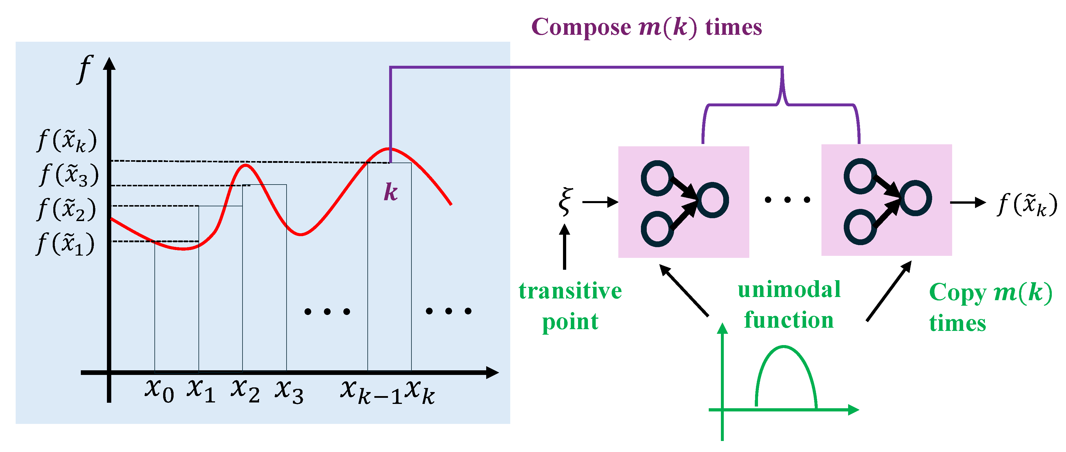
Figure 5.
A polynomial can be transformed into a unimodal map.
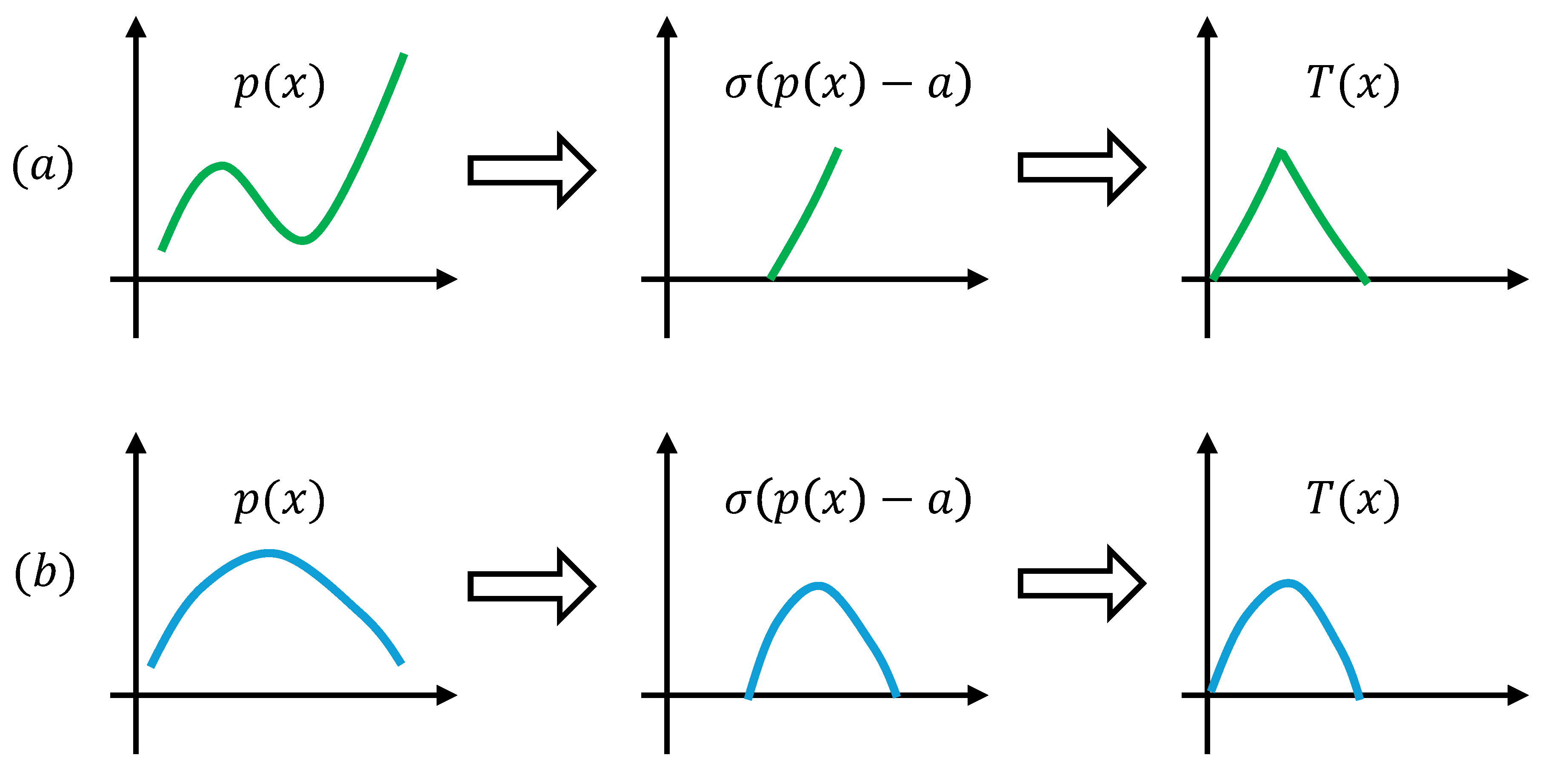
Figure 6.
Given a set U with , it will always contain a tiny subset such that . Then, naturally , since .
Figure 6.
Given a set U with , it will always contain a tiny subset such that . Then, naturally , since .
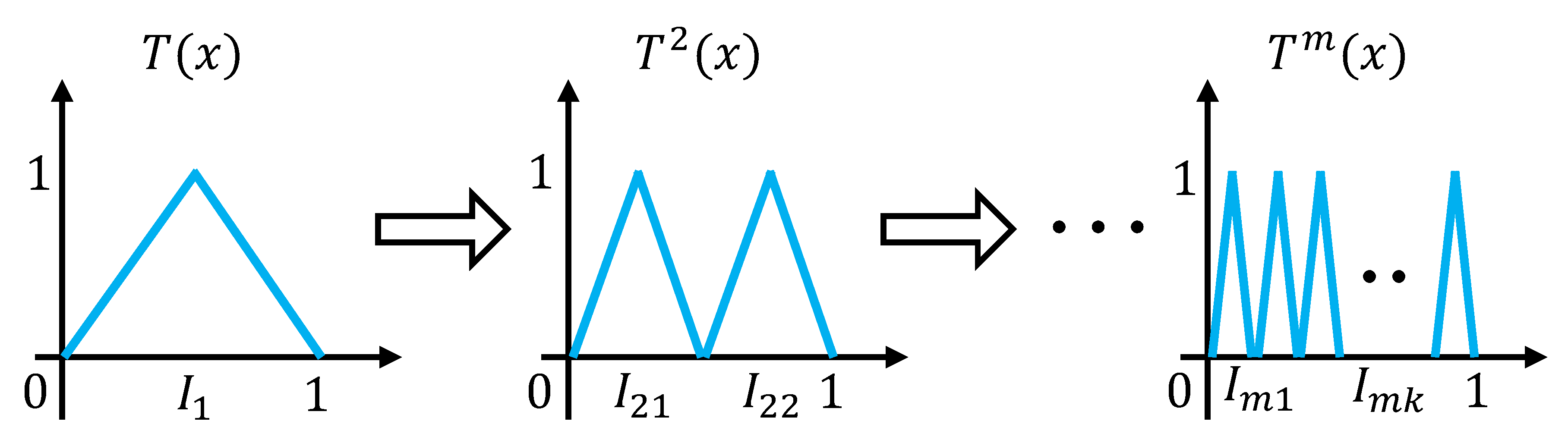
Figure 7.
The uniqueness experiment on phoneme data.
Figure 8.
Uniqueness experiment on airfoil self-noise data.
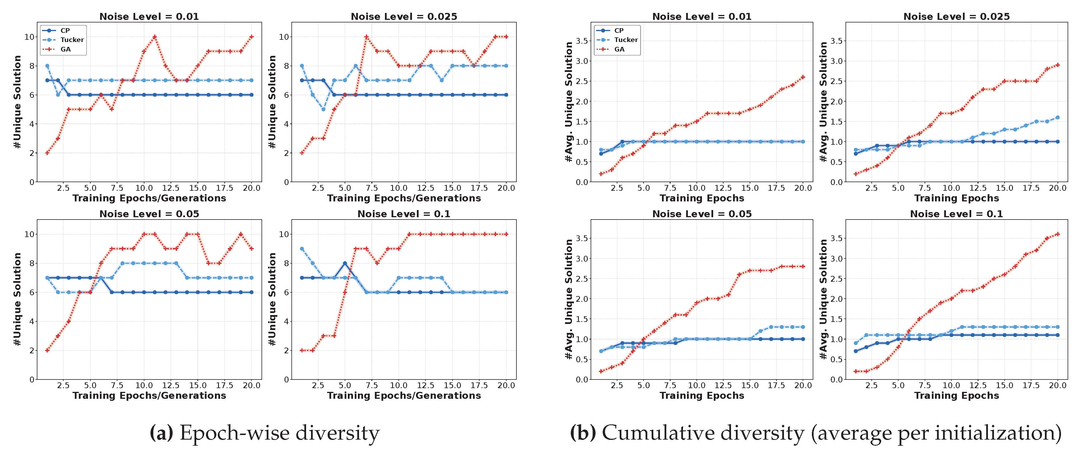
Figure 9.
Comparison between CP and Tucker decomposition. (a) Performance comparison on regression tasks measured by MSE. (b) Performance comparison on classification tasks measured by accuracy.
Figure 9.
Comparison between CP and Tucker decomposition. (a) Performance comparison on regression tasks measured by MSE. (b) Performance comparison on classification tasks measured by accuracy.
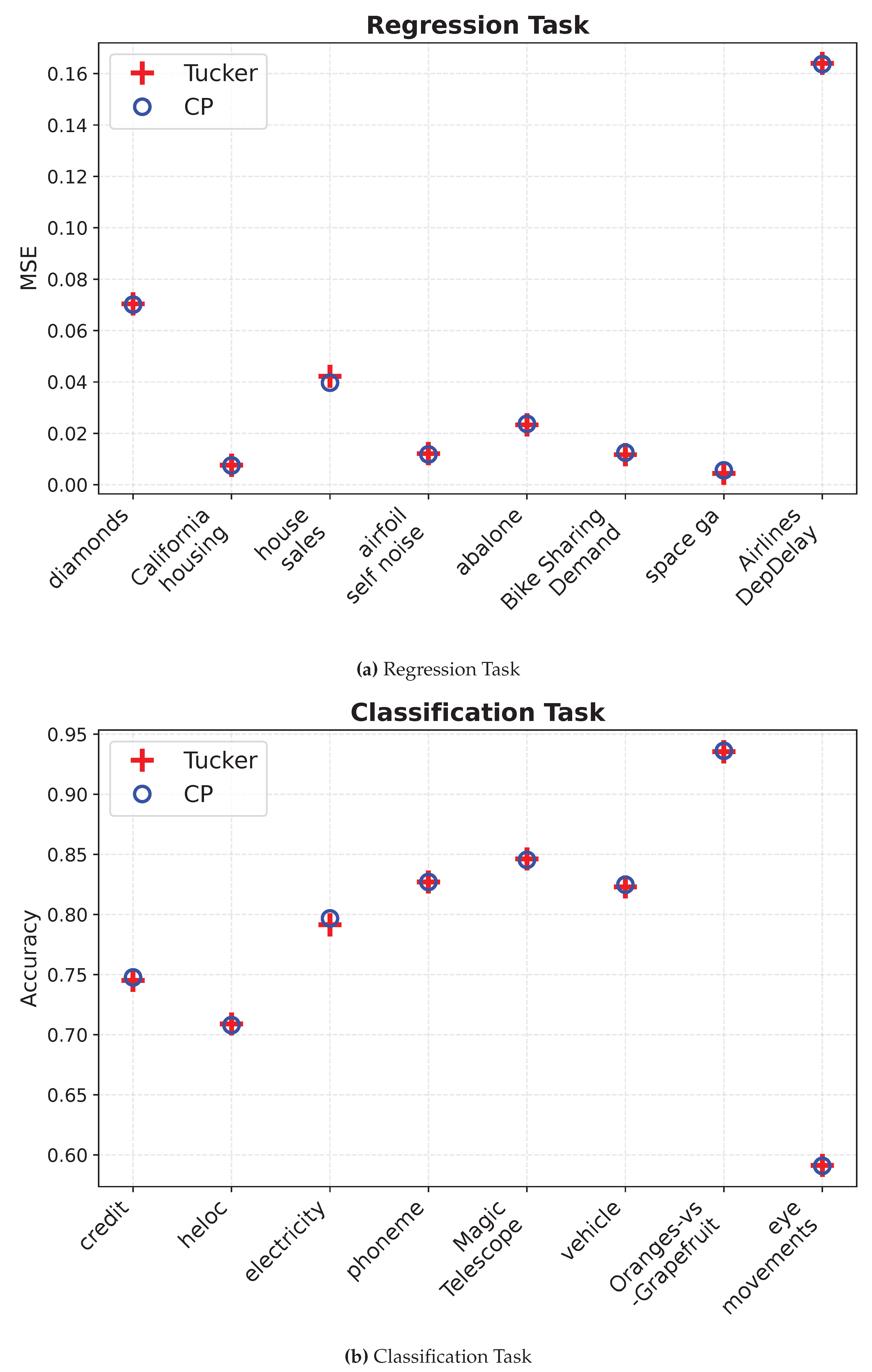
Figure 10.
Comparison between CP and Tucker decomposition
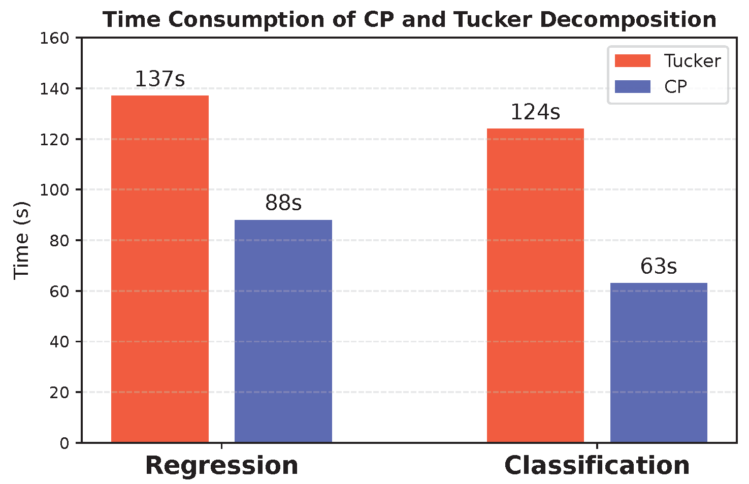

Table 1.
A summary of the recently-proposed neurons. is the nonlinear activation function. ⊙ denotes Hadamard product. , , and the bias terms in these neurons are omitted for simplicity.
Table 1.
A summary of the recently-proposed neurons. is the nonlinear activation function. ⊙ denotes Hadamard product. , , and the bias terms in these neurons are omitted for simplicity.
| Works | Formulations |
|---|---|
| Zoumponuris et al. (2017) [25] | |
| Fan et al. (2018) [30] | |
| Jiang et al. (2019) [26] | |
| Mantini & Shah (2021) [27] | |
| Goyal et al. (2020) [28] | |
| Bu & Karpante (2021) [29] | |
| Xu et al. (2022) [9] | |
| Fan et al. (2024) [12] | Task-driven polynomial |
Table 2.
Regression results (MSE) on synthetic data. represents the noise level.
| Ground Truth Formula | Time (s) | |||||||
|---|---|---|---|---|---|---|---|---|
| SR | TD | SR | TD | SR | TD | SR | TD | |
| 0.0013 | 0.0008 | 0.0108 | 0.0120 | 0.0232 | 0.0138 | 13.94 | 4.46 | |
| 0.0007 | 0.0006 | 0.0163 | 0.0095 | 0.0191 | 0.0166 | 12.75 | 6.69 | |
| 0.0235 | 0.0028 | 0.2489 | 0.0102 | 0.1905 | 0.1706 | 28.77 | 7.73 | |
| 0.0016 | 0.0012 | 0.0139 | 0.0101 | 0.0147 | 0.0116 | 22.01 | 8.82 | |
| 0.0095 | 0.0067 | 0.0116 | 0.0086 | 0.0495 | 0.0064 | 15.16 | 5.80 | |
| 0.0011 | 0.0002 | 0.0230 | 0.0165 | 0.0561 | 0.0193 | 24.77 | 9.44 | |
| 0.0055 | 0.0014 | 0.0125 | 0.0104 | 0.0416 | 0.0109 | 15.80 | 8.21 | |
| 0.0102 | 0.0062 | 0.0134 | 0.0111 | 0.0170 | 0.0126 | 13.30 | 8.24 | |
Table 3.
Comparison of the network built by neurons using formulas generated by NeuronSeek-SR and NeuronSeek-TD. The number means that this network has k hidden layers, each with neurons. For example, 5-3-1 means this network has two hidden layers with 5 and 3 neurons respectively in each layer.
Table 3.
Comparison of the network built by neurons using formulas generated by NeuronSeek-SR and NeuronSeek-TD. The number means that this network has k hidden layers, each with neurons. For example, 5-3-1 means this network has two hidden layers with 5 and 3 neurons respectively in each layer.
| Datasets | Instances | Features | Classes | Metrics | Structure | Test results | ||
|---|---|---|---|---|---|---|---|---|
| TN | NeuronSeek-TD | NeuronSeek-SR | NeuronSeek-TD | |||||
| California housing | 20640 | 8 | continuous | MSE | 6-4-1 | 6-3-1 | 0.0720 ± 0.0024 | 0.0701 ± 0.0014 |
| house sales | 21613 | 15 | continuous | 6-4-1 | 6-4-1 | 0.0079 ± 0.0008 | 0.0075 ± 0.0004 | |
| airfoil self-noise | 1503 | 5 | continuous | 4-1 | 3-1 | 0.0438 ± 0.0065 | 0.0397 ± 0.0072 | |
| diamonds | 53940 | 9 | continuous | 4-1 | 4-1 | 0.0111 ± 0.0039 | 0.0102 ± 0.0015 | |
| abalone | 4177 | 8 | continuous | 5-1 | 4-1 | 0.0239 ± 0.0024 | 0.0237 ± 0.0027 | |
| Bike Sharing Demand | 17379 | 12 | continuous | 5-1 | 5-1 | 0.0176 ± 0.0026 | 0.0125 ± 0.0146 | |
| space ga | 3107 | 6 | continuous | 2-1 | 2-1 | 0.0057 ± 0.0029 | 0.0056 ± 0.0030 | |
| Airlines DepDelay | 8000 | 5 | continuous | 4-1 | 4-1 | 0.1645 ± 0.0055 | 0.1637 ± 0.0052 | |
| credit | 16714 | 10 | 2 | ACC | 6-2 | 6-2 | 0.7441 ± 0.0092 | 0.7476 ± 0.0092 |
| heloc | 10000 | 22 | 2 | 18-2 | 17-2 | 0.7077 ± 0.0145 | 0.7089 ± 0.0113 | |
| electricity | 38474 | 8 | 2 | 5-2 | 5-2 | 0.7862 ± 0.0075 | 0.7967 ± 0.0087 | |
| phoneme | 3172 | 5 | 2 | 8-5 | 7-5 | 0.8242 ± 0.0207 | 0.8270 ± 0.0252 | |
| MagicTelescope | 13376 | 10 | 2 | 6-2 | 6-2 | 0.8449 ± 0.0092 | 0.8454 ± 0.0079 | |
| vehicle | 846 | 18 | 4 | 10-2 | 10-2 | 0.8176 ± 0.0362 | 0.8247 ± 0.0354 | |
| Oranges-vs-Grapefruit | 10000 | 5 | 2 | 8-2 | 7-2 | 0.9305 ± 0.0160 | 0.9361 ± 0.0240 | |
| eye movements | 7608 | 20 | 2 | 10-2 | 10-2 | 0.5849 ± 0.0145 | 0.5908 ± 0.0164 | |
Table 4.
Details of real-world tabular datasets.
| Dataset | Task | Data Size | Features |
|---|---|---|---|
| Electron Collision Prediction | Regression | 99,915 | 16 |
| Asteroid Prediction | Regression | 137,636 | 19 |
| Heart Failure Detection | Classification | 1,190 | 11 |
| Stellar Classification | Classification | 100,000 | 17 |
Table 5.
The test results of different models on real-world datasets.
| Method | electron collision (MSE) | asteroid prediction (MSE) | heartfailure (F1) | Stellar Classification (F1) |
|---|---|---|---|---|
| XGBoost | 0.0094 ± 0.0006 | 0.0646 ± 0.1031 | 0.8810 ± 0.02 | 0.9547 ± 0.002 |
| LightGBM | 0.0056 ± 0.0004 | 0.1391 ± 0.1676 | 0.8812 ± 0.01 | 0.9656 ± 0.002 |
| CatBoost | 0.0028 ± 0.0002 | 0.0817 ± 0.0846 | 0.8916 ± 0.01 | 0.9676 ± 0.002 |
| TabNet | 0.0040 ± 0.0006 | 0.0627 ± 0.0939 | 0.8501 ± 0.03 | 0.9269 ± 0.043 |
| TabTransformer | 0.0038 ± 0.0008 | 0.4219 ± 0.2776 | 0.8682 ± 0.02 | 0.9534 ± 0.002 |
| FT-Transformer | 0.0050 ± 0.0020 | 0.2136 ± 0.2189 | 0.8577 ± 0.02 | 0.9691 ± 0.002 |
| DANETs | 0.0076 ± 0.0009 | 0.1709 ± 0.1859 | 0.8948 ± 0.03 | 0.9681 ± 0.002 |
| NeuronSeek-SR | 0.0016 ± 0.0005 | 0.0513 ± 0.0551 | 0.8874 ± 0.05 | 0.9613 ± 0.002 |
| NeuronSeek-TD (ours) | 0.0011 ± 0.0003 | 0.0502 ± 0.0800 | 0.9023 ± 0.03 | 0.9714 ± 0.001 |
Table 6.
Accuracy of compared methods on small-scale image datasets.
| CIFAR10 | CIFAR100 | SVHN | STL10 | |
|---|---|---|---|---|
| ResNet18 | 0.9419 | 0.7385 | 0.9638 | 0.6724 |
| NeuronSeek-ResNet18 | 0.9464 | 0.7582 | 0.9655 | 0.7005 |
| DenseNet121 | 0.9386 | 0.7504 | 0.9636 | 0.6216 |
| NeuronSeek-DenseNet121 | 0.9399 | 0.7613 | 0.9696 | 0.6638 |
| SeResNet101 | 0.9336 | 0.7382 | 0.9650 | 0.5583 |
| NeuronSeek-SeResNet101 | 0.9385 | 0.7720 | 0.9685 | 0.6560 |
| GoogleNet | 0.9375 | 0.7378 | 0.9644 | 0.7241 |
| NeuronSeek-GoogleNet | 0.9400 | 0.7519 | 0.9658 | 0.7298 |
Disclaimer/Publisher’s Note: The statements, opinions and data contained in all publications are solely those of the individual author(s) and contributor(s) and not of MDPI and/or the editor(s). MDPI and/or the editor(s) disclaim responsibility for any injury to people or property resulting from any ideas, methods, instructions or products referred to in the content. |
© 2025 by the authors. Licensee MDPI, Basel, Switzerland. This article is an open access article distributed under the terms and conditions of the Creative Commons Attribution (CC BY) license (http://creativecommons.org/licenses/by/4.0/).
Copyright: This open access article is published under a Creative Commons CC BY 4.0 license, which permit the free download, distribution, and reuse, provided that the author and preprint are cited in any reuse.


