Submitted:
17 June 2025
Posted:
17 June 2025
You are already at the latest version
Abstract
According to all of the test points, the least squares method is used to conduct regression of the soil shear strength index. The regression residual has variance and correlation, which reduces the effectiveness of the regression strength index and increases the variance. To eliminate the variance and correlation of the regression residuals, in this paper, we employ variable substitution of the explanatory variables, explained variables, and residual vector, that is, the square root matrix of the original residual covariance matrix on both sides of the original regression equation, so that the residuals of the new regression equation have homogeneity of variance and no correlation and thus meet the application conditions of the least squares method. The mean and variance of the shear strength indexes are estimated for triaxial consolidated drained (CD) tests on breccia rockfill, triaxial unconsolidated undrained (UU), CD, and consolidated undrained (CU) tests on gravel clay, and triaxial CD tests on sandy soil. The results show that in general, the mean value of the shear strength index estimated using the generalized least squares method is not very different from that obtained using the traditional method, but the average standard deviation of the cohesion is reduced by 30.575% and the average standard deviation of the friction angle is reduced by 14.21%, which significantly improves the estimation accuracy of the shear strength index of soil.
Keywords:
Mohr–Coulomb shear strength of soil
; generalized least squares method
; mean value
; variance
1. Introduction
In geotechnical engineering, the shear strength of soil is mostly determined by the Mohr–Coulomb strength formula, and the strength indicators, namely, the cohesion and friction angle, are important design parameters. The determination of the foundation bearing capacity, verification of soil slope stability, design of retaining structures, correctness of indicator values, and their discreteness all directly affect the safety and economy of a project.
At present, most current standards adopt the partial factor limit state design method based on reliability theory for structural design. The material properties need to consider adverse variations on their standard values. The standard value of the material performance is generally taken as a percentile value of the probability distribution of the material performance. The material strength is generally taken as a lower percentile value of the probability distribution, except for the mean values of the elastic modulus and Poisson’s ratio at the 0.5th percentile. As is commonly employed internationally, the 0.05th percentile is taken (GB 50068-2018). If the material strength follows a normal distribution, the standard value of the material strength is , where and are the mean and standard deviation of the material strength.
According to the Unified Standard for Reliability Design of Water Resources and Hydropower Engineering Structures (GB50199-2013), the standard value for the strength of rock and soil materials and their artificial foundations can adopt the 0.1th percentile value (GB 5099-2013), and the strength standard value is . According to the Design Code for Rolled Earth Rock Dams in China (NB/T10872-2021), the soil strength index (11 groups, 4–6 samples per group) should be calculated using the average of the small values (NB/T 10872-2021) and the equation. According to the Code for the Investigation of Geotechnical Engineering (GB50021-2001 (2009 edition)), the standard values of the shear strength of rock and soil are calculated as follows: and . is the mean value of shear strength indicator, and is the statistical correction factor (GB 50021-2001). is the sample size. is the coefficient of variation of the shear strength index, and . is the standard deviation of the shear strength index. Therefore, the determination of the standard deviation of the soil shear strength index and the mean of the index are equally important (GB/T 50123-2019).
At present, the shear strength index of a rock and soil mass is usually determined using fitting regression method, and the most commonly used methods include the moment method, least squares method, point group center method, and optimal slope method. Based on a great deal of sampling and experimentation, the application of the moment method or linear regression, two mathematical statistical methods, to determine the shear strength index is currently the most commonly used and accurate method. However, in general, the sample size of each group of experiments is relatively small, and the moment method is greatly affected by experimental errors and human factors. The least squares linear regression method places the experimental points of each group in the same coordinate system for regression calculation, which not only effectively solves the problem of the sample size but also eliminates the errors contained in the cohesion and friction angle obtained from each group of experiments. Although the linear regression method has the characteristics of a large sample size and high accuracy, the standard deviation obtained is not a true reflection of the variability of the actual shear strength index, which has often been overlooked in previous calculations.
The classic least squares method is used to determine the shear strength index of soil, and the estimated values of the and indices are unbiased. The main reason for the large error in the variance estimation is that the regression equation does not meet the adaptation conditions of the least squares method. In other words, the residuals between the measured and predicted values of the regression equation have variance anisotropy and correlation. Least squares regression requires the residuals to be independent and to follow a normal distribution with a mean of zero and equal variance. However, the regression results of triaxial tests on soil samples indicate that the residuals in the regression equation have heteroscedasticity and are correlated with each other. The heteroscedasticity and correlation of regression residuals render parameter estimators ineffective as the variances are not constant and interrelated, rendering t-tests and F-tests ineffective. Due to the influence of the variance of each component of the parameter, the fluctuation between the estimated and true values of the parameter increases, which reduces the estimation accuracy, and as a result, the parameter variance estimated using the least squares method is no longer the minimum variance estimate. Because the variance of the random error term and the variance of the parameter estimator are included in the prediction variance, the variance of the explained variable increases under the influence of the increase in the variance of the parameter estimator, and thus, it reduces the prediction accuracy of the explained variable. Clearly, the variance estimation of the shear strength parameter index is too large, which will lead to fluctuation of the calculation results for geotechnical buildings, a poor grasp of the safety of the geotechnical buildings in the calculation, and the unreasonable design of geotechnical buildings in terms of economy.
Therefore, it is of great practical significance to reasonably determine the mean and variance of the shear strength index of soil so that designers can more accurately grasp the shear strength index and improve the reliability of calculations. The way to solve this problem is to eliminate the variance and correlation of the residuals in the regression equation.
2. Method for Organizing the Shear Strength Parameters of Soil
The method: indoor triaxial testing is one of the main methods for determining the shear strength of soil. The stress difference at the failure of the specimen under various confining pressures of is obtained from the triaxial test. According to the Mohr–Coulomb strength formula, the failure line equation is as follows:
where is the major principal stress at the time of sample failure, is the minor principal stress, and are the cohesive force and friction angle of soil shear strength, and and are undetermined coefficients. They can be calculated by the following formulas:, and .
It can be seen that regression Equation (1) cannot directly obtain the and indexes of the soil shear strength, but they are determined by the intermediate variables of and . They are calculated as follows:
where and are obtained through linear regression of n experimental points in Equation (1).
According to Equation (1) and probability theory, the following equation can be obtained through derivation:
where is the variance of the principal stress, and and are the standard deviations of the regression parameters and , respectively.
By performing Taylor expansion on Equation (2) at the mean values of and while ignoring second-order and higher-order infinitesimal quantities, the corresponding variance expressions for and can be obtained:
Therefore,
Chen et al. (2005) pointed out that it is clear from both theoretical derivation and analysis of experimental results that the shear strength parameter values obtained using the method and the method are not the same. Their analysis suggests that the difference between the two is caused by the error of , and it is believed that the results of the method are more accurate. Yu et al. (2012) used the orthogonal least squares method to modify the shear strength parameters of the regression method for soil. They derived the revised regression coefficients. It has been theoretically proven that the shear strength parameter values obtained using the modified method are consistent with those obtained using the method, and a practical example has also verified that the and values obtained using these two methods are the same. However, the impacts of the variance and correlation of the regression residuals of the method on the regression results were not considered. Chen et al. (2007) used the weighted least squares method to organize the shear strength of 64 sets of 320 triaxial consolidated drained (CD) test results for the core wall material of the Xiaolangdi dam. The weighting coefficient used was calculated using the equation , and the parameters were obtained through linear regression of the residuals and independent variables. This is actually equivalent to partially considering the variance heterogeneity of the residuals without fundamentally solving the problem, and no discussion on eliminating the residual correlation has been published (Phoon, 2017; Tomobe et al., 2021; Zhao et al., 2017; Zambrano et al., 2003).
3. Classic Least Squares Estimation (Wang et al., 2021; Douglas et al., 2022)
Assuming that is the dependent variable, is the independent variable that affects , there is a linear relationship between and , and there are n sets of observed values (xi,yi), i = 1, 2, 3…, n, then
where is the residual term, which represents the influence of factors other than on and the experimental measurement error. and are unknown parameters that need to be estimated.
If the residual term of satisfies the following conditions: (a) it is expected to be zero, ; (b) equal variance ; and (c) if there is no correlation () between the residuals, then the least squares estimation holds. This is the Gauss–Markov condition.
The matrix expression of the linear regression model is
where , , , and denotes the transpose of the matrix. is the identity matrix, and is the variance of the entire residual sequence.
The least squares method is used to obtain an estimate of the parameter β, which minimizes the sum of the squared lengths of the error vector of , i.e.,
This equation is expanded, the partial derivative is calculated and set to zero, and the parameters to be estimated are calculated as follows:
By substituting n sets of observation data into the above equation, the estimated value of β, i.e.,, is obtained.
The covariance matrix of the parameter is as follows:
4. Variance Homogeneity and Independence Test of Regression Residuals for Principal Stress Expressions with Large and Small Sample Damage
The criterion for determining the homogeneity of the variance and the correlation of the regression residuals depends on the covariance matrix of the regression residuals. If all of the diagonal elements of the covariance matrix are equal, the regression residuals have homogeneity of variance; otherwise, they have heteroscedasticity. If the non-diagonal elements of the covariance matrix are not all zero, then the regression residuals are correlated. If all of the non-diagonal elements are zero, then the residuals under different confining pressures are uncorrelated. To calculate the regression residual matrix, it is necessary to first regress the experimental data. The calculation process of the regression failure principal stress relationship and the regression residual covariance matrix based on the three-axis test results is described below.
Based on the results of triaxial tests on soil, the principal stress at the failure points of soil samples under different confining pressures is determined, and n sets of regression data of are generated. Then, the classical least squares method is used to regress the relationship between the large and small principal stresses at the point of failure, and the regression coefficients and are obtained. Then, the cohesion and friction angle of the soil are calculated using Equation (2).
The results of the large triaxial tests on the coarse-grained gravel soil material of project R, the small triaxial CD, unconsolidated undrained (UU), and consolidated undrained (CU) tests on the gravel clay material of project S, and the small triaxial tests on the sandy soil of project T are obtained. Classic least squares regression is performed on the large principal stress and small principal stress at the point of failure (Figure 1, Figure 3, Figure 5, Figure 7 and Figure 9). After obtaining the regression equation, the difference between the measured values of the principal stress at failure and the values predicted via regression is calculated and taken as the residual. The regression residuals of the five tests on the three types of soil materials mentioned above are presented in Figure 2, Figure 4, Figure 6, Figure 8 and Figure 10.
Figure 1.
Least squares regression of the principal stress for the coarse-grained breccia soil.
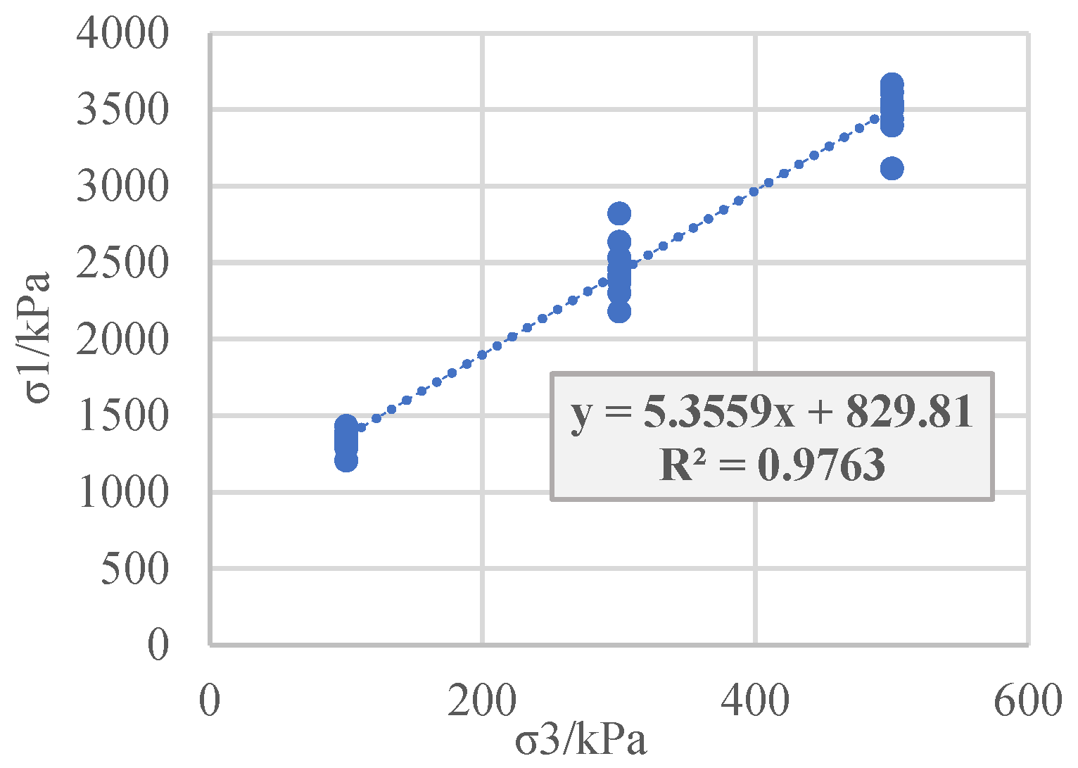
Figure 2.
Residual least squares regression for the coarse-grained breccia soil.
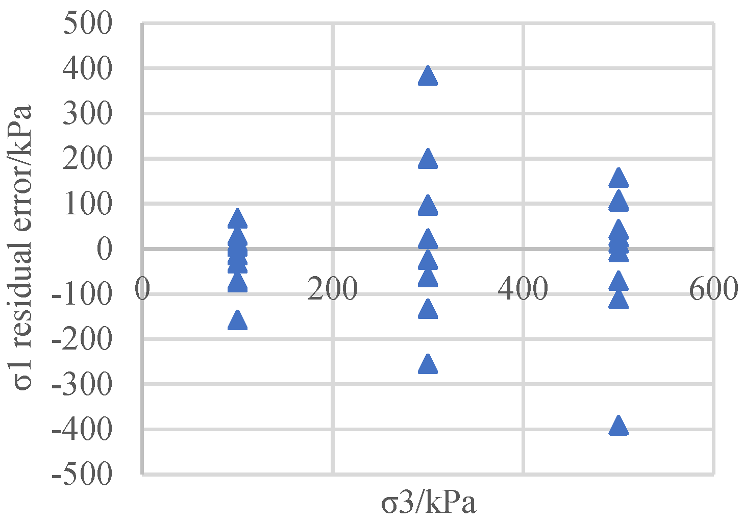
Figure 3.
Least squares regression of the principal stress for the CD test on gravel clay material.
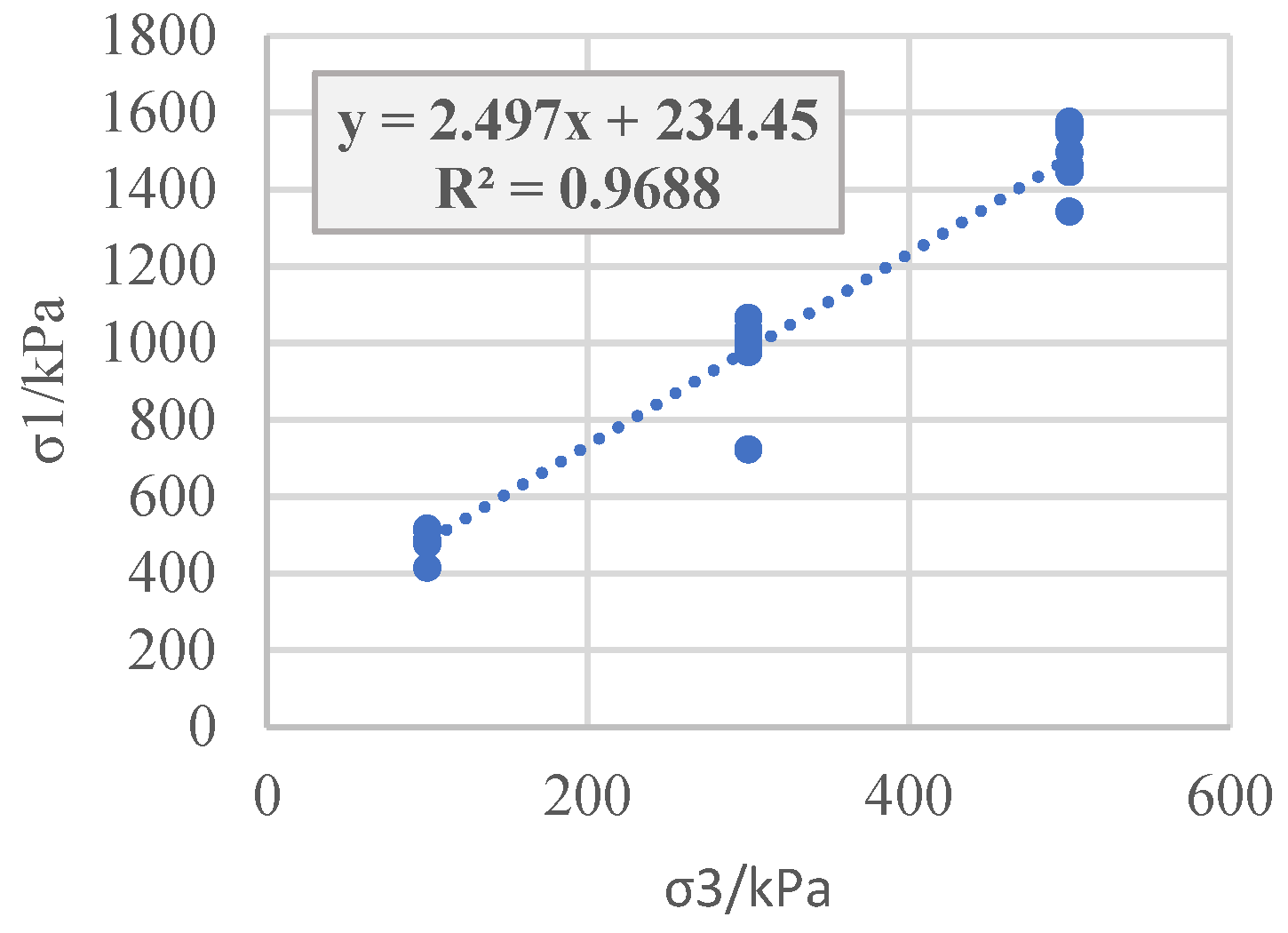
Figure 4.
Regression residuals for the CD test on the gravel clay material.
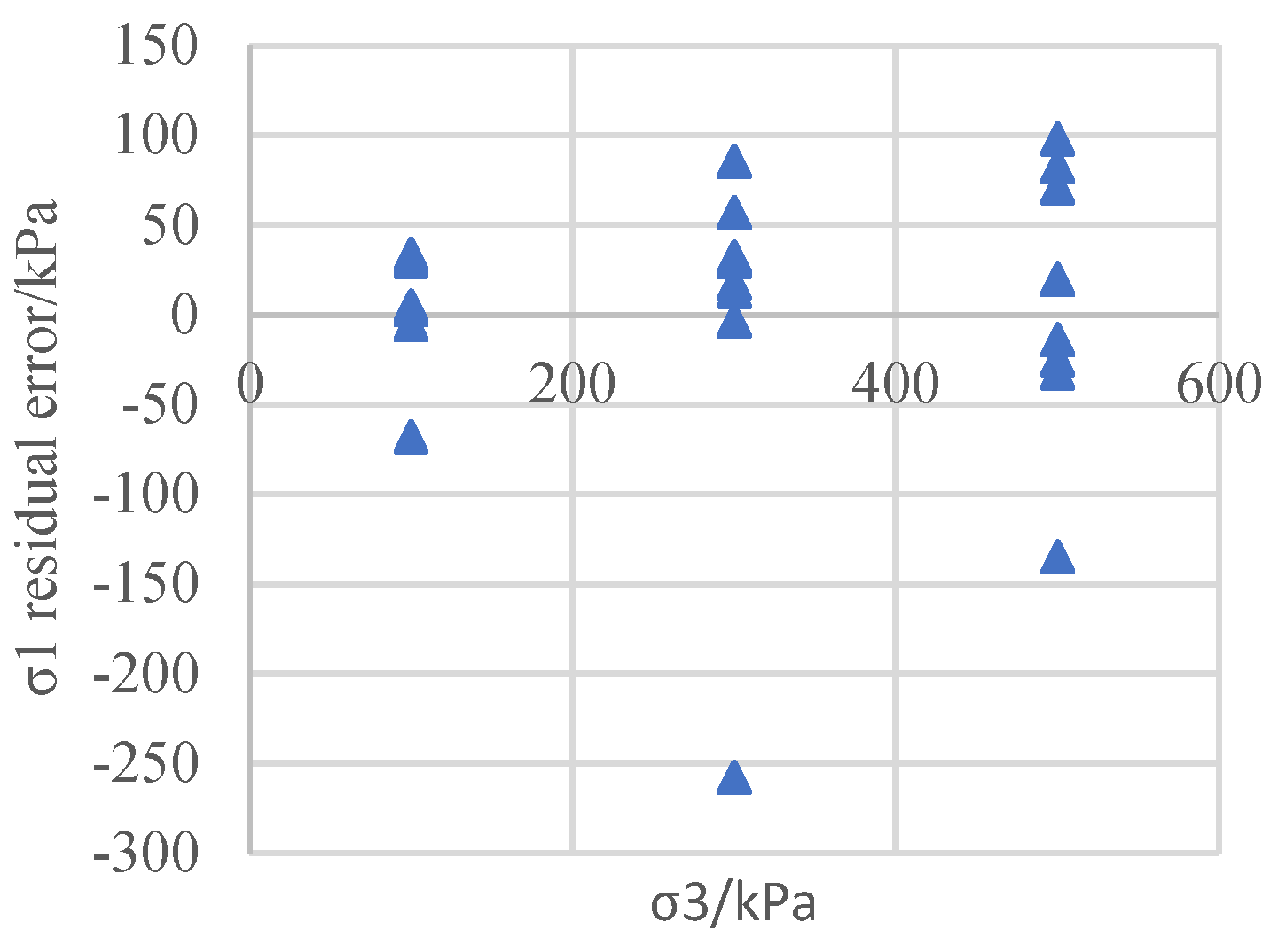
Figure 5.
Least squares regression of the principal stress for the UU test on the gravel clay material.
Figure 5.
Least squares regression of the principal stress for the UU test on the gravel clay material.
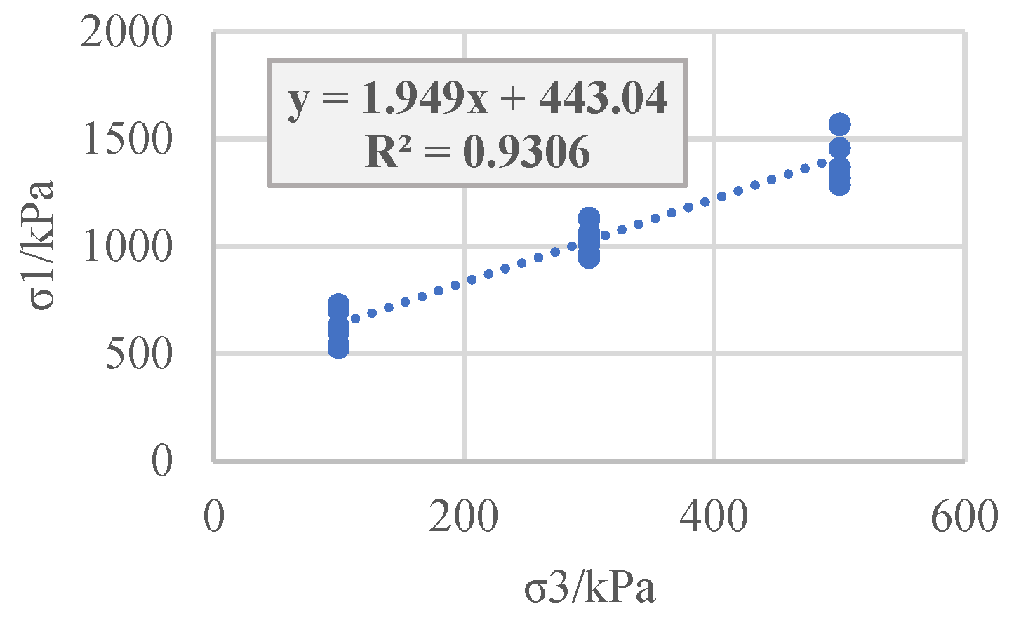
Figure 6.
Regression residuals for the UU test on the gravel clay material.
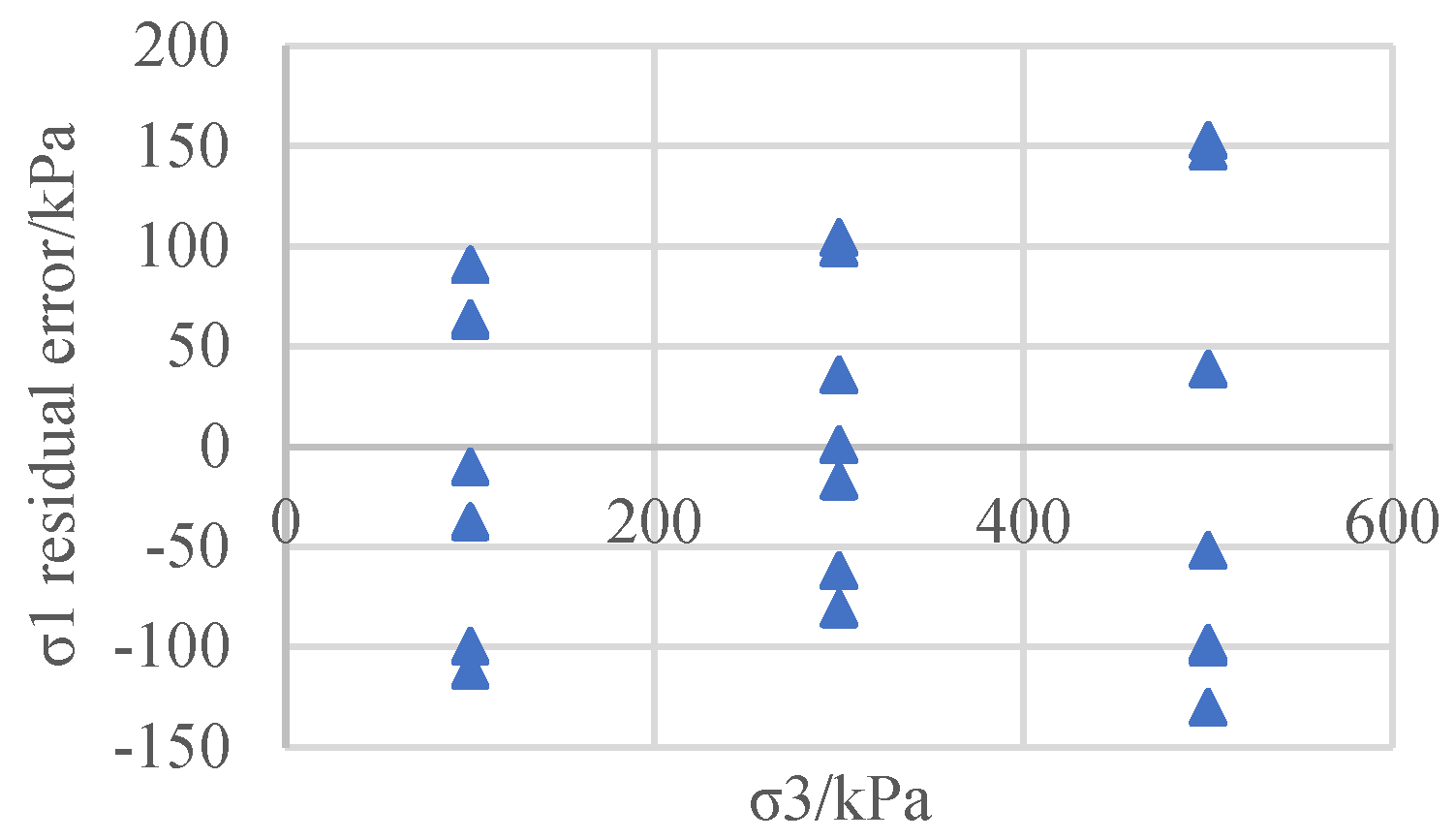
Figure 7.
Least squares regression of the principal stress for the CU test on the gravel clay material.
Figure 7.
Least squares regression of the principal stress for the CU test on the gravel clay material.

Figure 8.
Regression residuals for the CU test on the gravel clay material.
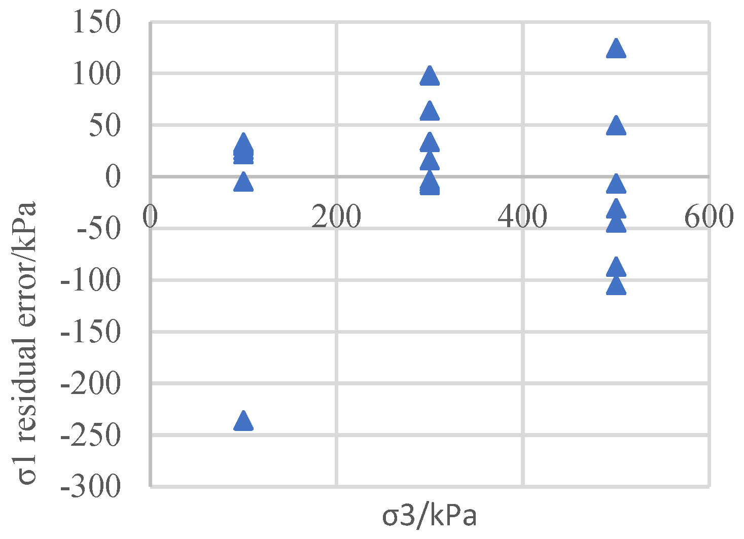
Figure 9.
Least squares regression of the principal stress for the small triaxial CD test on the sand soil.
Figure 9.
Least squares regression of the principal stress for the small triaxial CD test on the sand soil.
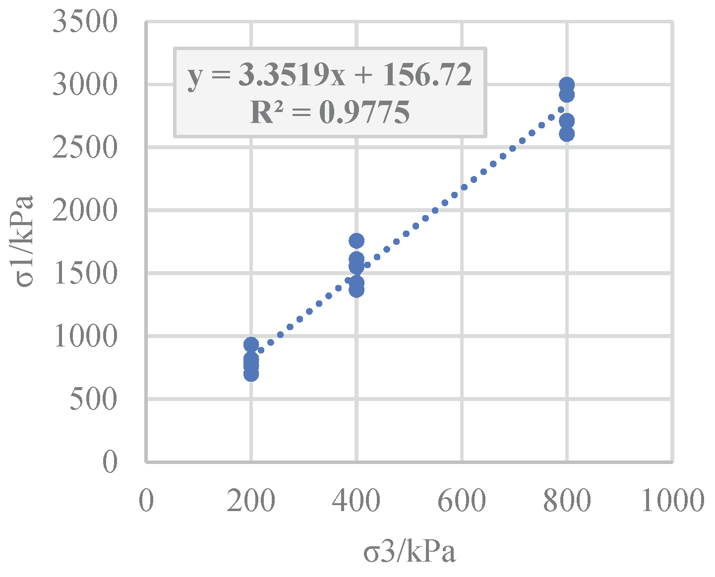
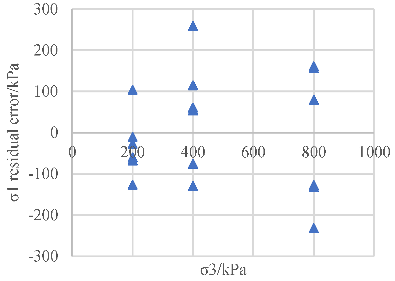
Figure 10.
Regression residuals for the small triaxial CD test on the sandy soil.
The covariance matrix of the residuals under different confining pressures is calculated for the three types of soil materials and five different tests as follows. For the coarse-grained breccia soil, the covariance matrix of the classical least squares linear regression residuals is as follows:
where .
Therefore,
For the gravelly clay material, the covariance matrix of the classic least squares regression residuals and the CD test is as follows.
where .
Therefore,
For the gravel clay material, the covariance matrix of the residual of the classic least squares regression and the UU test is as follows:
where .
Therefore,
For the gravelly clay material, the covariance matrix of the classic least squares regression residuals and the UU test is as follows:
where .
Therefore,
For the sandy soil, the covariance matrix of the residuals of the classic least squares linear regression is as follows:
where .
Therefore,
As can be seen from Figures 2, 4, 6, 8, and 10, the distribution of the regression residuals is not the same under different confining pressures. For the same soil material and test, some of the residual points of the confining pressure are relatively concentrated, while others are scattered, indicating that the residuals under different confining pressures do not have homogeneity of variance. Based on the regression covariance matrices of the different types of soil test results, the covariance matrix is full rank, the diagonal elements are unequal, and the non-diagonal elements are not zero, indicating that the residuals not only have variance anisotropy but also correlation.
The above examples illustrate that for coarse-grained soil, sandy soil, and cohesive soil, for both the effective stress intensity index of the CD test and the total strength index of the UU and CU tests, when using the least squares method for soil shear strength parameter regression, the residuals have variance and correlation. If the classic least squares method is used to conduct the estimation, its parameters will no longer be valid, and the significance test of the variables and he model prediction will all experience a certain degree of failure. Therefore, efforts should be made to improve the classic least squares regression method in order to adapt it to the heteroscedasticity of the shear strength residuals and eliminate the correlation of the residuals.
5. Eliminating Residual Variance Heterogeneity and Correlation Using the Generalized Least Squares Method (Wang et al., 2021; Douglas et al., 2022)
When the soil is destroyed, the linear regression equation of the relationship has the following properties:
where it is nonsingular and positive definite, and there is a nonsingular symmetric matrix , so . Matrix is the square root matrix of , and and are the transpose matrix and inverse matrix of .
Multiplying both sides of the regression equation by at the same time yields :
Thus, the regression variation is as follows:
After this process, the error of the model has a mean value of zero, i.e., , and the covariance matrix of is calculated as follows:
Therefore, the element of has the properties of a mean value of zero, constant variance, and no correlation. The test conditions of the classical least squares estimation are satisfied, and the least squares function is calculated as follows:
Its canonical equation is as follows:
The solution of this equation is as follows:
The covariance of is as follows:
6. Example Calculation
Eleven groups of triaxial test data for coarse-grained breccia soil material for project R were used, and the confining pressures of each group were set to six levels. Considering the nonlinearity of the shear strength of the coarse-grained soil, the Mohr–Coulomb shear strength was divided into multiple sections. Here, only the shear strength of the low confining pressure section with three levels of confining pressure (100 kPA, 300 kPa, and 500 kPa) are discussed. Eleven groups of small triaxial UU, CD and CU tests were also carried out on the gravelly clay materials for project S. However, due to certain differences in the dry density of the samples, seven groups of test data with similar densities were selected for calculation. The confining pressures for each group of tests were 100 kPA, 300 kPa, and 500 kPa. Six groups of CD tests were carried out on sand for project T, and the confining pressure scores of each group of tests were also divided into three levels, i.e., 200 kPa, 400 kPa, and 800 kPa.
The covariance matrix (Equation (14)) of the regression parameters and of the classic least squares method is the covariance matrix of the regression parameters obtained under the Gauss–Markov condition. However, when regressing the relationship of the soil triaxial test using the classic least squares method, its residual does not meet the Gauss–Markov condition, and its covariance matrix of parameter can be modified as follows:
The friction angle and cohesion of the soil shear strength can be calculated using Equation (2) after and are calculated using classic and generalized least squares methods according to Equations (13) and (21). Then, the variance and covariance of the friction angle and cohesion are calculated using Equations (2)–(7). The specific calculations are presented in Table 1 and Table 2. Table 1 shows the regression parameters and their variance calculation. It can be seen that both the variances of and and the covariance between and are smaller for the generalized least squares method than the classic least squares method, indicating that the generalized least squares method is better than the classic least squares method.

Table 1.
Least squares regression parameters of and and the variance.
| Soil quality | method | Variance difference of residuals | Residual correlation | |||||
| Project R, engineering coarse-grained soil, CD | classic | 829.81 | 5.3559 | 8361.866 | 0.0935 | −6.657 | exists | exists |
| generalized | 807.24 | 5.3396 | 3940.604 | 0.0923 | −4.346 | eliminated | eliminated | |
| Project S, engineering gravelly clay material, UU | classic | 443.04 | 1.949 | 6206.01 | 0.0253 | 2.767 | exists | exists |
| generalized | 448.41 | 1.977 | 4220.19 | 0.0094 | 0.272 | eliminated | eliminated | |
| Project S, engineering gravelly clay material, CD | classic | 234.45 | 2.497 | 2132.80 | 0.0190 | 1.3909 | exists | exists |
| generalized | 240.55 | 2.504 | 429.45 | 0.0166 | −0.6206 | eliminated | eliminated | |
| Project S, engineering gravelly clay material, CU | classic | 211.3 | 2.2783 | 17806.65 | 0.1376 | −44.09 | exists | exists |
| generalized | 282.3 | 2.1453 | 7198.30 | 0.0805 | −21.37 | eliminated | eliminated | |
| Project T, engineering sand, small triaxial CD | classic | 156.72 | 3.352 | 4026.72 | 0.0361 | 2.2829 | exists | exists |
| generalized | 149.42 | 3.289 | 3950.93 | 0.0304 | 1.6266 | eliminated | eliminated |
Table 2.
Soil shear strength, cohesion, and friction angle and their variance, standard deviation, and coefficient of variation.
Table 2.
Soil shear strength, cohesion, and friction angle and their variance, standard deviation, and coefficient of variation.
| Soil quality | method | (kPa) | Friction angle (°) | Variance of | Variance of (10-2 radians) | Covariance of and | Standard deviation of | Standard deviation of (°) | Coefficient of variation of | Coefficient of variation of |
| Project R, engineering coarse-grained soil, CD | classic | 179.28 | 43.26 | 464.64 | 0.0432 | −0.204 | 21.56 | 1.191 | 0.120 | 0.028 |
| generalized | 174.67 | 43.20 | 239.94 | 0.043 | −0.167 | 15.49 | 1.188 | 0.089 | 0.028 | |
| Project S, engineering gravelly clay material, UU | classic | 158.67 | 18.77 | 757.38 | 0.15 | −0.010 | 27.52 | 2.22 | 0.173 | 0.118 |
| generalized | 159.46 | 19.16 | 541.33 | 0.05 | − .068 | 23.27 | 1.33 | 0.146 | 0.070 | |
| Project S, engineering gravelly clay material, CD | classic | 74.18 | 25.35 | 204.65 | 0.06 | 0.0286 | 14.306 | 1.429 | 0.193 | 0.0564 |
| generalized | 76.00 | 25.42 | 52.65 | 0.05 | −0.081 | 7.256 | 1.332 | 0.095 | 0.0523 | |
| Project S, engineering gravelly clay material, CU | classic | 69.995 | 22.95 | 2435.1 | 0.56 | −3.378 | 49.346 | 4.295 | 0.705 | 0.187 |
| generalized | 96.366 | 21.35 | 1207.1 | 0.38 | −2.278 | 34.743 | 3.528 | 0.361 | 0.165 | |
| Project T, engineering sand, small triaxial CD | classic | 42.800 | 32.71 | 293.8 | 0.06 | 0.0494 | 17.14 | 1.366 | 0.401 | 0.042 |
| generalized | 41.197 | 32.25 | 295.9 | 0.05 | 0.0332 | 17.20 | 1.284 | 0.418 | 0.040 |
It can be seen from Table 2 that for all three soil materials (i.e., coarse-grained soil, sandy soil, and gravelly clay) and for all of the test types (i.e., UU, CD, and CU triaxial tests and large and small triaxial tests), the shear strength index of soil obtained using the generalized least squares method eliminates the variance and correlation of the residuals is not significantly different from that obtained using the classic least squares method, but the standard deviation obtained using the generalized least squares method is generally smaller. The generalized least squares method improves the accuracy of the soil shear strength estimation, which is of great significance for accurately determining the safety of geotechnical engineering projects.
There are two points to be noted in the calculation results, as follows.
(a) As can be seen from Table 2, for the total strength and cohesion from the small triaxial CU test on the gravelly clay material in the three projects, there is a certain difference between the results of the two calculation methods, with a value of 69.995 kPa obtained using the classic least squares method and a value of 96.366 kPa obtained using the generalized least squares method. This is because the test has a low outlier at 100 kPa (Figure 7 and Figure 8). In mathematics, the classic least squares method takes the minimum residual error as the objective function, and this low outlier will inevitably lower the regression intercept of , the classical least squares, and the generalized least squares of . Therefore, the robust regression of the soil shear strength by the generalized least squares method is better than that of the classic least squares method. According to Equation (2), the cohesion index of soil is directly proportional to the regression intercept, so the cohesion determined using the classic regression least squares method is low.
(b) As can be seen from Table 2, for the standard deviation of the cohesion of the sand for project T, there is little difference between the values obtained using the generalized and classic least squares regression methods, with values of 17.14 and 17.20 kPa, respectively, but that obtained from the generalized least squares method is slightly larger. This is because there is little difference between the two methods regarding the regression parameter , with values of 4026.72 and 3950.93 for the generalized and classic least squares regression methods, respectively. The variance of the regression parameter obtained using the generalized least squares method is lower. However, due to the inconsistency between the regression parameters and the variance conversion multiple of the cohesion, the final standard deviation of the cohesion is slightly larger.
Table 3 shows the variation in the standard deviation of the Mohr–Coulomb shear strength index between the classic least squares method and the generalized least squares method. It can be seen that except for the 0.4% increase in the standard deviation of the cohesion of the sand soil, the other standard deviations are reduced. The standard deviation of the cohesion is reduced by 28–49.3% (average of 30.575%), and the standard deviation of the friction angle is reduced by 0.25–40.1% (average of 14.21%). It can be seen that the generalized least squares method eliminates the variance difference, and the correlation of the residuals has an obvious effect on reducing the standard deviation of the Mohr–Coulomb shear strength index.
7. Conclusions
The shear strength of soil is an important parameter in geotechnical engineering. The selection of the cohesion and internal friction angle index has a direct impact on determining the bearing capacity of the foundation, checking the stability of the soil slope, and designing retaining structures. Most of current codes stipulate that the shear strength of soil is a low quantile value of the probability distribution. For example, the unified standard for structurally reliable design of water conservancy and hydropower projects (GB 50199-2013) stipulates that the standard value of the strength of geotechnical materials and artificial foundations can be 0.1 quantile value, and its standard strength value is , where and are the mean and standard deviation of the material strength. Therefore, the determination of the standard deviation of the soil shear strength index is equally important.
At present, the triaxial test is the main test method used to determine the shear strength of soil. The method and the method are mostly used for the finishing parameters. The method is based on the p and q value regression linear model, and the equation is used to obtain the parameters C and D. Then, the friction angle and cohesion of the soil are calculated using the following formulas: , and . This method is a method for determining the shear strength specified in some specifications. Because the independent variable and dependent variable are random variables, it does not meet the condition that in the linear regression, the independent variable is not a random variable, which directly affects the accuracy of the shear strength parameter estimation. The method regresses the linear model using the equation according to the values of N-groups of failure points, and then, it calculates the friction angle and cohesion of the soil using Equation (2). In this study, based on the classic least squares regression of the results of UU, CD, and CU triaxial tests on coarse-grained soil, sandy soil, and cohesive soil, it was found that the regression residuals have heteroscedasticity and correlation. This does not meet the premise of using the least squares method, and the friction angle and cohesion index variances obtained using this method do not reflect the variability of the actual shear strength.
In order to eliminate the variance difference and the correlation of the regression residuals, a generalized least squares regression method for soil shear strength was developed in this study. In other words, the explanatory variable, dependent variable, and residual vector of the regression equation are replaced by variables, and the square root matrix of the covariance matrix of the original residual is multiplied on both sides of the original regression equation. Thus, the residual of the new regression equation is homogeneous and uncorrelated, so it conforms to the application conditions of the least squares method. Based on triaxial CD tests on coarse-grained soil and sand and UU, CD and CU tests on gravelly clay, the shear strength parameters and their variances are estimated. In this study, it was found that the variance of the shear strength parameters estimated using the generalized least squares method was lower when the change in the shear strength parameters was small. In the calculation example presented in this paper, the standard deviation of the cohesion was reduced by 30.575% on average, and the standard deviation of the friction angle was reduced by 14.21% on average, which improved the accuracy of the estimation of the shear strength parameters of the soil.
Acknowledgements
This work is supported in part by the Project funded by the National Science Foundation of China (52379116), and. The opinions and findings presented are those of the writers and do not necessarily reflect the views of the sponsor. We thank LetPub (www.letpub.com.cn) for its linguistic assistance during the preparation of this manuscript.
Declaration of competing interest
The authors declare that they have no known competing financial interests or personal relationships that could have appeared to influence the work reported in this paper.
Abbreviations
The abbreviations and symbols in this paper are presented below.
| Mean value of soil material strength | |
| Standard deviation of soil material strength | |
| Mean value of soil shear strength index | |
| Statistical correction factor | |
| Number of samples | |
| Variation coefficient of shear strength index | |
| Standard deviation of shear strength index | |
| Cohesiveness | |
| Friction angle | |
| Maximum principal stress at specimen failure | |
| Minimum principal stress at specimen failure | |
| Variance of maximum principal stress | |
| Standard deviation of β0 | |
| Standard deviation of | |
| Residual term | |
| Identity matrix | |
| Variance of the entire residual sequence | |
| Least squares method for estimating parameters | |
| Least squares method for estimating parameters | |
| Estimated value of | |
| Square root matrix of | |
| Transposition matrix of | |
| Inverse matrix of |
References
- Chen, L., CHEN, Z., LI, G., 2005. Discussion of linear regression method to estimate shear strength parameters from results of triaxial tests. Rock and Soil Mechanics. 26: 1785-1789.
- Chen, L., CHEN Z., LI, G., 2007, A modified linear regression method to estimate shear strength parameters. Rock and Soil Mechanics. 28: 1421-1426.
- Douglas, C., Mentgomery, E., Peck, G., 2022. Introduction to Linear Regression Analysis (Fifth Edition), Beijing: China machine Press.
- GB 50068-2018. Unified Standard for Reliability Design of Building Structures. Ministry of Housing and Urban-Rural Development of the People’s Republic of China, Standardization Administration of the People’s Republic of China. Beijing: China Architecture & Building Press.
- GB 5099-2013. Unified Standard for Reliability Design of Hydraulic Engineering Structures. Ministry of Water Resources of the People’s Republic of China. Beijing: China Water & Hydropower Press.
- GB 50021-2001. Code for Investigation of Geotechnical Engineering (2009 Edition). Ministry of Housing and Urban-Rural Development of the People’s Republic of China. Beijing: China Architecture & Building Press.
- GB/T 50123-2019. Standard for Geotechnical Testing Methods. Ministry of Housing and Urban-Rural Development of the People’s Republic of China. Beijing: China Architecture & Building Press.
- Lai, Y., Gao, Z., G., Zhang, S., Chang, X., 2010. Stress-strain relationships and nonlinear mohr strength criteria of frozen sandy clay. Soils and Foundations, 50: 45-53.
- NB/T 10872-2021. Design Code for Rolled Earth-rock Fill Dams. National Energy Administration of the People’s Republic of China. Beijing: China Electric Power Press.
- Phoon, K., 2017. Role of reliability calculations in geotechnical design. Georisk, 11: 4-21. [CrossRef]
- Tomobe, H., Fujisawa, K., Murakami, A., 2021. A Mohr-Coulomb-Vilar model for constitutive relationship in root-soil interface under changing suction. Soils and Foundations, 61: 815-835. [CrossRef]
- Wang, G., Chen, Min., Chen, L., 2021. Linear statistical model - linear regression and variance analysis. Beijing Higher Education Press.
- Yu, D., Yao, H., Wu, S., 2012. Difference and modification of regression analysis methods to estimate shear strength parameters obtained by triaxial test[J]. Rock and Soil Mechanics, 33: 3037-3042.
- Zambrano, M., Valko, P., Russell, J., 2003. Error-in-variables for rock failure envelope. International Journal of Rock Mechanics and Mining Sciences, 40: 137-143.
- Zhao, L.-H., Cheng, X., Dan, H.-C., Tang, Z.-P., Zhang, Y., 2017. Effect of the vertical earthquake component on permanent seismic displacement of soil slopes based on the nonlinear Mohr–Coulomb failure criterion. Soils and Foundations, 57: 237-251. [CrossRef]
Table 3.
Percentage reduction of the standard deviation of the soil shear strength index after eliminating the residual variance and correlation.
Table 3.
Percentage reduction of the standard deviation of the soil shear strength index after eliminating the residual variance and correlation.
| method | Gravelly clay, UU | Gravelly clay, CD | Gravelly clay, CU | ||||||
| classic | generalized | variation | classic | generalized | variation | classic | generalized | variation | |
| (kPa) | 27.52 | 23.27 | 15.4 | 14.306 | 7.256 | 49.3 | 49.346 | 34.743 | 29.6 |
| (°) | 2.22 | 1.33 | 40.1 | 1.429 | 1.332 | 6.8 | 4.295 | 3.528 | 17.9 |
| metho | Sandy soil, CD | Coarse-grained breccia soil | Average decrease | ||||||
| classic | generalized | variation | classic | generalized | variation | ||||
| (kPa) | 17.14 | 17.20 | −0.4 | 21.56 | 15.49 | 28 | 30.575 | (kPa) | 17.14 |
| (°) | 1.366 | 1.284 | 6 | 1.191 | 1.188 | 0.25 | 14.21 | (°) | 1.366 |
Disclaimer/Publisher’s Note: The statements, opinions and data contained in all publications are solely those of the individual author(s) and contributor(s) and not of MDPI and/or the editor(s). MDPI and/or the editor(s) disclaim responsibility for any injury to people or property resulting from any ideas, methods, instructions or products referred to in the content. |
© 2025 by the authors. Licensee MDPI, Basel, Switzerland. This article is an open access article distributed under the terms and conditions of the Creative Commons Attribution (CC BY) license (http://creativecommons.org/licenses/by/4.0/).
Copyright: This open access article is published under a Creative Commons CC BY 4.0 license, which permit the free download, distribution, and reuse, provided that the author and preprint are cited in any reuse.


