
Submitted:
14 June 2025
Posted:
17 June 2025
You are already at the latest version
Abstract
This paper presents a new Bayesian inverse framework improved by convolutional adaptation for the numerical approximation of weakly singular Volterra integral equations. The proposed methodology addresses the computational difficulties associated with singular kernels by implementing a convolution-based regularization technique that makes the kernel easier to deal with. A prior Gaussian process with a radial basis function kernel is used, together with a gradual mesh transformation that concentrates the quadrature points near the singularities, significantly improving numerical accuracy without compromising efficiency. Numerical experiments confirm the robustness and efficiency of the method in various scenarios, demonstrating strong convergence and stability in various hyperparameter configurations. Our approach outperforms existing methods in comparative benchmarks with collocation and Legendre wavelet probes.
Keywords:
Volterra equation
; kernels
; inverse problems
; Gaussian processes
; adaptive quadrature
1. Introduction
Volterra’s integral equations, named after Vito Volterra [1,2], constitute a fundamental class where the unknown function appears under an integral with variable limits. These equations model systems with memory effects across physics, biology, economics, and control theory [3,4].
The mathematical foundations were established by pioneering work of Volterra [3,4], Lalescu [5], Fredholm [6], and Hilbert [7], with later contributions from Wiener and Hopf [8,9], Taylor [10], and Kato [11].
Volterra equations are classified into first-kind and second-kind equations. While continuous kernels allow direct treatment, singular or weakly singular kernels pose considerable challenges due to their divergent behavior [12,13,14]. The theory was extensively developed by Tricomi [15], Muskhelishvili [16], and Erdélyi [17].
Existing solution methods include analytical approaches such as Laplace transforms [18,19], series solutions [20,21], and Picard iteration [22], alongside numerical methods including quadrature methods [23,24], collocation methods [13,25,26], and Galerkin methods [27,28]. Specialized techniques for singular kernels involve graded meshes [29,30] and product integration [31,32].
Traditional methods face significant limitations, especially regarding stability and uncertainty quantification near singularities. Conventional methods often fail near singularities, producing unreliable results due to inherent ill-conditioning and error propagation. Current techniques lack robust uncertainty management and adaptive strategies for handling singular behavior.
This study proposes an innovative hybrid approach combining Bayesian inference with Gaussian processes and adaptive convolutional regularization to solve Volterra integral equations with weak singularities. Our methodology addresses traditional limitations by exploiting Gaussian processes’ uncertainty quantification capabilities while utilizing regularization techniques to stabilize numerical behavior near singularities, enhanced by importance sampling [33] and logarithmic stabilization methods [34].
This paper is organized as follows: in Section 2, we provide a detailed description of the proposed method. In Section 3, we deal with the numerical examples and we conclude in Section 4.
2. Proposed Method
We consider the singular Volterra integral equation of the second kind defined by:
where represents the unknown function, while , , and F are given functions. The parameter is a scalar multiplier, and determines the type and strength of the singularity.
The Volterra operator is formally defined as:
where represents the singular kernel. For , the exponent creates a weak singularity, and the integral
remains convergent, ensuring the well-posedness of the problem. Existence and uniqueness for similar singular kernels are discussed in [35,36].
2.1. Bayesian Formulation
2.1.1. Likelihood Function
2.1.2. Prior Distribution
2.1.3. Posterior Distribution
2.2. Singularity Treatment
The primary computational challenge lies in handling the singularity [35,36] when as . We propose a convolutional regularization approach:
where is a small adaptive regularization parameter that prevents numerical overflow while preserving the singular behavior. The associated local regularization error is defined by:
For , this error admits the expansion:
By binomial expansion with , we have:
Using the Taylor expansion:
Substituting u and simplifying yields the desired expansion. We then define the relative regularization error as:
Furthermore, if the error in the data is , then the propagated error in the solution satisfies the bound:
This relationship demonstrates that values of that are too small amplify data errors.
To concentrate quadrature points near the singularity, we employ a graded mesh transformation:
with to increase point density near . The adaptive weights [35,41] are defined as:
where C and are positive parameters that enhance accuracy near the singular point. The local density of quadrature points is characterized by the spacing between consecutive points:
Using the mean value theorem, there exists such that:
We define the relative density of points near the singularity as:
Indeed, for , , and for , . Therefore, . This relationship demonstrates that the larger becomes, the greater the concentration of points near the singularity. For the singular integral
the quadrature error with the graded mesh transformation is given by:
This error satisfies the bound [13,30]
where , is a constant independent of n, and g is the function defined by with .
When we perform the transformation , we obtain and . The transformed integral becomes:
The singularity at has a modified order of , and the error depends on the regularity of the transformed integrand. We apply a uniform composite quadrature formula in s (trapezoid in this case), of order p (typically ). The error is proportional to:
By repeated derivation of we obtain that each derivative generates dominant terms of the type For these terms to remain bounded near , we require the most restrictive condition being for . Thus we need:
In the context , we see that the real order of convergence is:
Hence the origin of the bound The optimal convergence order is achieved for . This optimal value is obtained by maximizing the convergence exponent in Equation (16). The aim is to maximize the exponent:
If , then and if , then . However, the derivability bound restricts to . For , this gives:
Therefore, the tipping point where and the maximum derivability are equal is indeed
We then employ importance sampling by drawing samples from the prior and weighting them by the likelihood. The importance weight for sample i is:
To prevent numerical overflow in the exponential function, we apply log-space stabilization:
2.3. Posterior Approximation and Reconstruction
After computing the importance weights for all N prior samples , we normalize them:
The posterior distribution is then approximated by the weighted empirical distribution:
where denotes the Dirac delta function centered at .
The posterior mean function is computed as:
The posterior variance is given by:
For uncertainty quantification, we construct pointwise credible intervals. At each point x, we sort the weighted samples and compute the credible interval as:
where is the p-th weighted quantile of the posterior samples at point x and is the confidence level.
2.3.1. Convergence Assessment
The quality of the approximation can be assessed through several complementary metrics that provide insights into different aspects of the reconstruction performance. The Effective Sample Size (ESS) [37,38], defined as , serves as a crucial indicator of sampling efficiency. When the ESS is low, it suggests that the importance weights are poorly distributed, with only a few samples carrying most of the weight, thereby indicating poor sampling efficiency and potential numerical instability.
Additionally, residual analysis provides a direct measure of how well the reconstructed solution satisfies the original integral equation. The residual function quantifies the discrepancy between the observed data and the Volterra operator applied to the posterior mean. Small residuals across the domain indicate that the reconstructed solution provides a good fit to the integral equation, while large or systematic residuals may suggest inadequate prior specification or insufficient sampling.
Furthermore, the Monte Carlo Standard Error (MCSE) quantifies the uncertainty in our posterior estimates due to the finite sample approximation. Given by , this metric provides a measure of the precision of our posterior mean estimates. A decreasing MCSE with increasing sample size indicates convergence of the Monte Carlo approximation, while persistently large MCSE values suggest the need for additional samples or improved sampling strategies.
2.3.2. Proposed Algorithm
- Initialization: Set up the GP prior with chosen hyperparameters and discretization grid .
- Prior Sampling: Generate N function samples from the GP prior.
-
Likelihood Evaluation: For each sample :
- Compute using adaptive quadrature with graded mesh transformation
- Apply singularity regularization:
- Evaluate using the likelihood formula
- Weight Computation: Calculate importance weights with log-space stabilization:
-
Posterior Approximation: Normalize weights and compute posterior statistics:
- Posterior mean:
- Posterior variance:
- Reconstruction: Output the posterior mean as the solution estimate along with pointwise credible intervals for uncertainty quantification.
2.4. Convergence and Stability
Let be the space of continuous functions on equipped with the uniform norm . We define the weighted Sobolev space by:
where
We assume kernel regularity conditions, namely that the kernel satisfies: , for some constant , and .
For and the regularization , we have:
for , where depends only on .
Using Taylor expansion and the mean value theorem, for and , we have:
where . The result follows by estimating .
2.4.1. Monte Carlo Estimation and Stability Analysis
The Monte Carlo estimator of the posterior mean satisfies:
where C depends on , ℓ, and the problem parameters, but is independent of N. Using the variance decomposition:
By the Cauchy-Schwarz inequality and Gaussian process properties:
The strong law of large numbers applies since under our assumptions.
2.4.2. Stability with Respect to Data Perturbations
Let be two data functions with . Then the corresponding posterior means satisfy:
where C depends on the hyperparameters but not on . The log-likelihoods satisfy:
By continuity of the operator L on and compactness of the Gaussian process support, the result follows.
2.4.3. Minimax Risk Analysis
For the function class , the minimax risk satisfies:
where is a constant. Under the optimal choice of hyperparameters and with samples, our Bayesian estimator satisfies:
3. Numerical Examples
To validate the effectiveness of the proposed Bayesian approach and demonstrate its capability in handling weakly singular Volterra integral equations, we present a series of numerical experiments. These simulations are designed to assess the accuracy, convergence properties, and robustness of our method under various conditions. For the quadrature points, we calculate , using his optimal equation form in (17).
3.1. Example 1: Abel Integral Equation
We begin our numerical investigation with a classical Abel integral equation, which serves as a fundamental benchmark for methods dealing with weakly singular kernels. This example allows us to evaluate the performance of our Bayesian inverse approach against well-established analytical and numerical solutions.
We consider the following Abel integral equation [42] of the second kind:
This equation represents a specific instance of our general formulation with the parameter values , , and the right-hand side function . The kernel function and the nonlinear function , making this a linear Abel equation with a characteristic weak singularity of order at .
The choice of corresponds to the classical Abel kernel, which exhibits the typical square-root singularity that appears in numerous physical applications, including particle physics, plasma dynamics, and image reconstruction problems. This test case serves as an ideal benchmark for validating our numerical approach due to its analytical tractability. The exact solution of this equation is .
Figure 1 and Figure 2 showcases the compelling results obtained from our comprehensive numerical experiments for Example 1. The striking visual evidence presented in Figure 1 reveals an exceptional alignment between the approximate and exact solutions, providing unequivocal validation of our method’s remarkable effectiveness. This outstanding performance is further substantiated by the quantitative analysis in Table 1, where our approach demonstrates extraordinary precision with an average absolute error of merely a testament to the method’s superior computational accuracy.
To comprehensively evaluate the influence of the critical hyperparameters , C, , and , we conducted an extensive parametric study across diverse computational scenarios. Figure 2 provides crucial insights into the evolution of both mean squared error and residual norm as functions of . The results demonstrate a clear and consistent pattern: as the number of quadrature points increases, we observe a remarkable dual improvement in both solution accuracy and convergence behavior, highlighting the robust scalability of our approach.
The hyperparameter sensitivity analysis reveals fascinating computational dynamics. Table 2 demonstrates that increasing values lead to substantial MSE reduction, thereby significantly enhancing convergence characteristics. Similarly, Table 3 corroborates this trend for the parameter, indicating optimal performance tuning capabilities. However, Table 4 reveals the expected computational trade-off: while larger C values may offer certain advantages, they inevitably result in increased computational overhead a critical consideration for practical implementation.
Most importantly, the comparative analysis presented in Table 1 illustrates the comparative performance metrics, indicating improved accuracy of the proposed method across all test points. Our proposed technique consistently outperforms both the collocation method and the Legendre wavelet approach, achieving significantly lower absolute errors across all test cases. This decisive advantage unambiguously establishes the superior performance and enhanced reliability of our methodology compared to these well-established competing methods. The substantial error reduction achieved by our approach not only validates its theoretical foundations but also demonstrates its practical value for high-precision computational applications.
3.2. Example 2: Nonlinear Volterra Equation with Polynomial Right-Hand Side
To further evaluate the robustness and versatility of our Bayesian approach, we consider a more challenging nonlinear Volterra integral equation that incorporates both the characteristic weak singularity and a complex polynomial forcing term. This test case allows us to assess the method’s performance in handling nonlinear kernels while maintaining computational efficiency.
We examine the following nonlinear Volterra integral equation [42]:
The exact solution to this equation is known to be , which provides a clear benchmark for accuracy assessment. We implemented our Bayesian algorithm to solve this problem and conducted extensive numerical experiments to evaluate its performance across different parameter configurations.
The results showcased in Figure 3 and Figure 4 for Example 2 present an even more impressive demonstration of our method’s exceptional capabilities. The comprehensive analysis includes both the direct comparison between exact and approximate solutions (Figure 3) and the detailed performance evolution as a function of computational points (Figure 4). The visual inspection of Figure 3 reveals a virtually flawless correspondence between the exact solution and our method’s approximation a remarkable achievement that underscores the method’s extraordinary precision and reliability.
This exceptional visual agreement is powerfully reinforced by the quantitative metrics presented in Table 5, which demonstrates our approach’s outstanding computational excellence with an average absolute error reaching an impressive —representing a full order of magnitude improvement compared to Example 1. This exceptional accuracy level positions our method at the forefront of high-precision numerical techniques.
Consistent with our findings from Example 1, the comprehensive hyperparameter analysis reveals intriguing computational characteristics. Figure 4 corroborates our previous observations, confirming that convergence performance exhibits consistent enhancement as increases, thereby validating the method’s robust scalability across different problem domains.
Remarkably, the hyperparameter sensitivity analysis for Example 2 unveils a fascinating aspect of our method’s robustness. Table 6, Table 7 and Table 8 demonstrate that the MSE and maximum absolute error remain virtually unaffected by variations in the hyperparameters , C, and . This exceptional stability indicates that our method possesses inherent robustness against parameter fluctuations, with only marginal variations in computational time observed across different parameter configurations due to intermediate calculations that influence the overall computational overhead.
The definitive validation of our method’s supremacy emerges from the comprehensive comparative analysis presented in Table 5. Our proposed approach decisively outperforms all competing methodologies, consistently achieving the lowest absolute errors across all evaluation metrics. This comprehensive superiority not only validates the theoretical foundations of our approach but also establishes its undisputed dominance in the field of high-precision numerical computations, making it the method of choice for demanding computational applications.
3.3. Limitations
Despite the exceptional performance demonstrated by our approach, it is important to acknowledge certain limitations that define its current scope of application. First, the proposed method is specifically designed to handle Volterra integral equations with weak singularities () and has not been validated for strong singularity cases (), thereby restricting its applicability to this particular class of problems. Second, scalability considerations arise as increasing the number of samples N required for adequate convergence leads to substantial growth in computational cost, which becomes particularly challenging for high-dimensional problems. Finally, the importance sampling algorithm may experience weight degeneracy in ill-conditioned problems, where only a few samples carry the majority of the statistical weight, potentially compromising numerical stability and reliability of posterior estimates.
4. Conclusions
In this study, we have proposed a novel numerical approach for solving Volterra’s integral equations with weak singularities by approximating the singular kernel through convolutional regularization and employing RBF kernels within a Gaussian process prior framework. A graded mesh transformation technique was implemented to achieve strategic sampling that concentrates the quadrature points around the singular regions of the equation, thereby enhancing computational efficiency and accuracy.
The comprehensive numerical experiments conducted across multiple test cases have demonstrated the robustness and effectiveness of our proposed methodology. The results consistently show strong convergence properties, achieving remarkable accuracy with absolute errors ranging from to . These performance metrics validate the theoretical foundations of our approach and confirm its practical applicability for solving weakly singular Volterra’s integral equations.
Furthermore, our parametric studies revealed that the method exhibits stable behavior across various hyperparameter configurations, with the number of quadrature points being the most influential factor for convergence enhancement. The computational efficiency of the algorithm, combined with its high accuracy, makes it a valuable tool for practitioners dealing with singular integral equations in various scientific and engineering applications.
Future work will focus on extending the method to strongly singular Volterra equations, as well as exploring adaptive mesh refinement and automated hyperparameter tuning using machine learning.
References
- Volterra, V. Leçons sur la théorie mathématique de la lutte pour la vie; Gauthier-Villars, 1931.
- Brunner, H. Volterra Integral Equations: An Introduction to Theory and Applications; Cambridge University Press, 2017.
- Volterra, V. Sulla teoria delle equazioni differenziali lineari. Memorie della Società Italiana delle Scienze 1896, 6, 3–68. [Google Scholar] [CrossRef]
- Volterra, V. Leçons sur les équations intégrales et les équations intégro-différentielles; Gauthier-Villars, 1913.
- Lalescu, T. Sur les équations de Volterra. Annali di Matematica Pura ed Applicata 1911, 20, 1–133. [Google Scholar]
- Fredholm, E.I. Sur une classe d’équations fonctionnelles. Acta Mathematica 1903, 27, 365–390. [Google Scholar] [CrossRef]
- Hilbert, D. Grundzüge einer allgemeinen Theorie der linearen Integralgleichungen. Nachrichten von der Gesellschaft der Wissenschaften zu Göttingen 1904, pp. 49–91.
- Wiener, N. Tauberian theorems; Annals of Mathematics, 1931.
- Hopf, E. Ergodentheorie; Springer, 1939.
- Taylor, A.E. Introduction to functional analysis; Wiley, 1958.
- Kato, T. Perturbation theory for linear operators; Springer, 1966.
- Abel, N.H. Solution de quelques problèmes à l’aide d’intégrales définies. Magazin for Naturvidenskaberne 1823, 1, 55–68. [Google Scholar] [CrossRef]
- Brunner, H. Collocation Methods for Volterra Integral and Related Functional Differential Equations; Cambridge University Press, 2004.
- Gorenflo, R.; Vessella, S. Abel integral equations: analysis and applications; Springer, 1991.
- Tricomi, F.G. Integral equations; Interscience Publishers, 1957.
- Muskhelishvili, N.I. Singular integral equations; Noordhoff, 1953.
- Erdélyi, A. Tables of integral transforms; McGraw-Hill, 1954.
- Arfken, G.B.; Weber, H.J.; Harris, F.E. Mathematical Methods for Physicists; Academic Press, 2013.
- Debnath, L.; Bhatta, D. Integral transforms and their applications; CRC Press, 2014.
- Adomian, G. A review of the decomposition method in applied mathematics. Journal of Mathematical Analysis and Applications 1988, 135, 501–544. [Google Scholar] [CrossRef]
- Adomian, G. Solving frontier problems of physics: the decomposition method; Kluwer Academic Publishers, 1994.
- Picard, É. Mémoire sur la théorie des équations aux dérivées partielles et la méthode des approximations successives. Journal de Mathématiques Pures et Appliquées 1890, 6, 145–210. [Google Scholar]
- Press, W.H.; Teukolsky, S.A.; Vetterling, W.T.; Flannery, B.P. Numerical Recipes: The Art of Scientific Computing; Cambridge University Press, 1986.
- Stoer, J.; Bulirsch, R. Introduction to numerical analysis; Springer, 2002.
- de Boor, C. A practical guide to splines; Springer, 1978.
- Trefethen, L.N. Approximation theory and approximation practice; SIAM, 2013.
- Bownds, J.M.; Wood, B. On Numerically Solving Non-linear Volterra Equations with Fewer Computations. SIAM Journal on Numerical Analysis 1976, 13, 705–719. [Google Scholar] [CrossRef]
- Canuto, C.; Hussaini, M.Y.; Quarteroni, A.; Zang, T.A. Spectral methods in fluid dynamics; Springer, 2006.
- Brunner, H.; van der Houwen, P.J. The Numerical Solution of Volterra Equations; North-Holland, 1986.
- Lubich, C. Runge-Kutta theory for Volterra and Abel integral equations of the second kind; Vol. 41, 1983; pp. 87–102.
- Young, A. The numerical solution of integral equations. Proceedings of the Royal Society of London 1954, 224, 561–573. [Google Scholar] [CrossRef]
- Atkinson, K.E. A survey of numerical methods for the solution of Fredholm integral equations of the second kind; SIAM, 1976.
- Robert, C.P.; Casella, G. Monte Carlo statistical methods; Springer, 2004.
- Higham, N.J. Accuracy and stability of numerical algorithms; SIAM, 2002.
- Dehbozorgi, R.; Nedaiasl, K. Numerical Solution of Nonlinear Abel Integral Equations. arXiv 2021, arXiv:2001.06240. [Google Scholar]
- Ramazanova, M.I.; Gulmanova, N.K.; Omarova, M.T. On solving a singular Volterra integral equation. Filomat 2025, 39, 3647–3656. [Google Scholar]
- Dashti, M.; Stuart, A.M. The Bayesian Approach To Inverse Problems. arXiv 2013, arXiv:1302.6989. [Google Scholar]
- Randrianarisoa, T.; Szabo, B. Variational Gaussian Processes For Linear Inverse Problems. arXiv 2023, arXiv:2311.00663. [Google Scholar]
- Bai, T.; Teckentrup, A.L.; Zygalakis, K.C. Gaussian processes for Bayesian inverse problems associated with PDEs. arXiv 2023, arXiv:2307.08343. [Google Scholar]
- Titsias, M. Variational Learning of Inducing Variables in Sparse Gaussian Processes. Journal of Machine Learning Research 2009.
- Brunner, H. Volterra Integral Equations: An Introduction to Theory and Applications; Cambridge University Press, 2004.
- Khani, A.; Belalzadeh, N. Numerical solution of volterra integral equations with weakly singular kernel using legendre wavelet method. Mathematics and Computational Sciences 2025, 6, 160–169. [Google Scholar]
- Cardone, A.; Conte, D.; D’Ambrosio, R.; Beatrice, P. Collocation Methods for Volterra Integral and Integro-Differential Equations: A Review. Axioms 2018, 7, 45. [Google Scholar] [CrossRef]
Figure 1.
Comparison of exact and approximate solutions with .
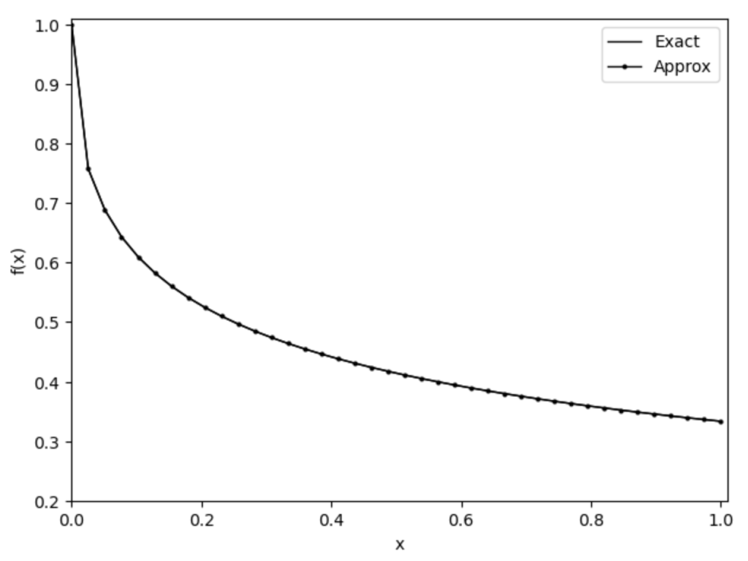
Figure 2.
Evolution of MSE and residual standard as a function of the total number of points considered.
Figure 2.
Evolution of MSE and residual standard as a function of the total number of points considered.
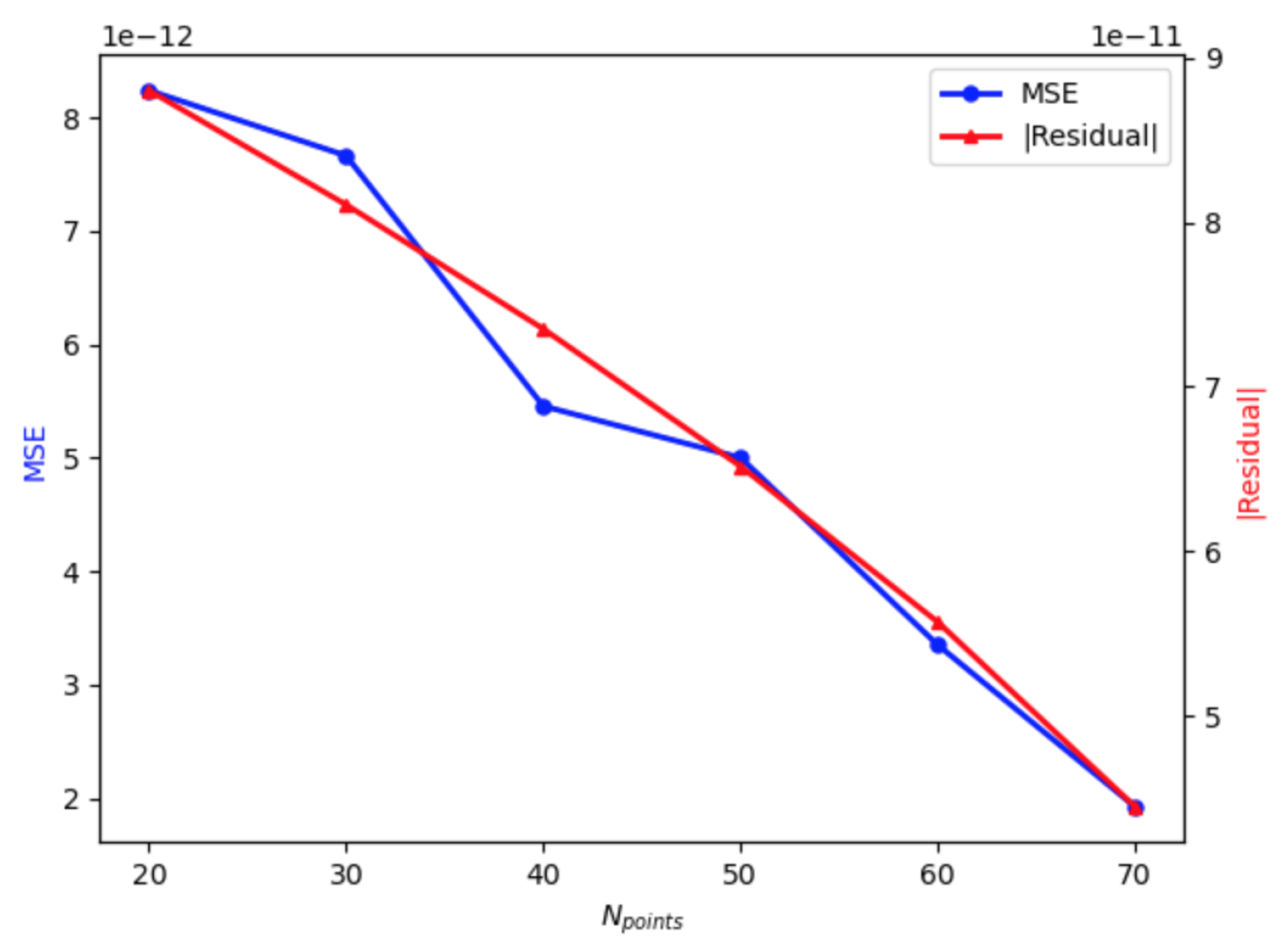
Figure 3.
Comparison of exact and approximate solutions with .
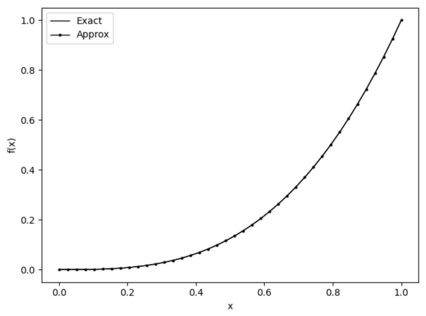
Figure 4.
Evolution of MSE and residual standard as a function of the total number of points considered.
Figure 4.
Evolution of MSE and residual standard as a function of the total number of points considered.


Table 1.
Comparison between our proposed method solution (Approx), collocation method, Legendre wavelet method and exact solution for example 1.
Table 1.
Comparison between our proposed method solution (Approx), collocation method, Legendre wavelet method and exact solution for example 1.
| x | Exact | Approx | Abs Err | Collocation [43] | Abs err | Wavelet [42] | Abs err |
|---|---|---|---|---|---|---|---|
| 0.1 | 0.612930 | 0.612933 | 0.608684 | 0.614358 | |||
| 0.2 | 0.528031 | 0.528032 | 0.527864 | 0.527519 | |||
| 0.3 | 0.477326 | 0.477325 | 0.477226 | 0.477342 | |||
| 0.4 | 0.441583 | 0.441582 | 0.441518 | 0.441461 | |||
| 0.5 | 0.414257 | 0.414255 | 0.414214 | 0.414252 | |||
| 0.6 | 0.392310 | 0.392309 | 0.392281 | 0.392246 | |||
| 0.7 | 0.374085 | 0.374083 | 0.374067 | 0.374108 | |||
| 0.8 | 0.358581 | 0.358583 | 0.358570 | 0.358509 | |||
| 0.9 | 0.345146 | 0.345145 | 0.345141 | 0.345250 | |||
| 1.0 | 0.333333 | 0.333333 | 0.333322 | 0.333251 |
Table 2.
Analysis of the performance and convergence metrics of the approximated solution for different values of for example 1.
Table 2.
Analysis of the performance and convergence metrics of the approximated solution for different values of for example 1.
| MSE | Max Abs Err | Runtime (s) | |
|---|---|---|---|
| 0.01 | 1.425 | ||
| 0.05 | 1.205 | ||
| 0.10 | 1.218 | ||
| 0.20 | 1.186 | ||
| 0.30 | 0.983 | ||
| 0.50 | 1.299 |
Table 3.
Analysis of the performance and convergence metrics of the approximated solution for different values of for example 1.
Table 3.
Analysis of the performance and convergence metrics of the approximated solution for different values of for example 1.
| MSE | Max Abs Err | Runtime (s) | |
|---|---|---|---|
| 1.0 | 1.660 | ||
| 5.0 | 1.726 | ||
| 10.0 | 2.222 | ||
| 15.0 | 2.472 | ||
| 20.0 | 2.165 | ||
| 30.0 | 1.730 |
Table 4.
Analysis of the performance and convergence metrics of the approximated solution for different values of C for example 1.
Table 4.
Analysis of the performance and convergence metrics of the approximated solution for different values of C for example 1.
| C | MSE | Max Abs Err | Runtime (s) |
|---|---|---|---|
| 1.0 | 1.084 | ||
| 5.0 | 1.006 | ||
| 10.0 | 1.913 | ||
| 15.0 | 1.296 | ||
| 20.0 | 1.735 | ||
| 30.0 | 2.030 |
Table 5.
Comparison between our proposed method solution (Approx), collocation method, Legendre wavelet method and exact solution for example 2.
Table 5.
Comparison between our proposed method solution (Approx), collocation method, Legendre wavelet method and exact solution for example 2.
| x | Exact | Approx | Abs Err | Collocation [43] | Abs err | Wavelet [42] | Abs err |
|---|---|---|---|---|---|---|---|
| 0.1 | 0.001017 | 0.001072 | 0.002087 | 0.000956 | |||
| 0.2 | 0.008061 | 0.008061 | 0.012741 | 0.007956 | |||
| 0.3 | 0.027123 | 0.027121 | 0.037091 | 0.026956 | |||
| 0.4 | 0.064189 | 0.064188 | 0.079570 | 0.063956 | |||
| 0.5 | 0.125247 | 0.125247 | 0.144281 | 0.124956 | |||
| 0.6 | 0.216285 | 0.216285 | 0.235123 | 0.215956 | |||
| 0.7 | 0.343291 | 0.343291 | 0.355847 | 0.342956 | |||
| 0.8 | 0.512254 | 0.512254 | 0.510098 | 0.511956 | |||
| 0.9 | 0.729161 | 0.729163 | 0.701431 | 0.728956 | |||
| 1.0 | 1.000000 | 0.999999 | 0.933333 | 0.999956 |
Table 6.
Analysis of the performance and convergence metrics of the approximated solution for different values of for example 2.
Table 6.
Analysis of the performance and convergence metrics of the approximated solution for different values of for example 2.
| MSE | Max Abs Err | Runtime (s) | |
|---|---|---|---|
| 0.01 | 1.839 | ||
| 0.05 | 0.768 | ||
| 0.10 | 0.970 | ||
| 0.20 | 0.860 | ||
| 0.30 | 0.922 | ||
| 0.50 | 1.181 |
Table 7.
Analysis of the performance and convergence metrics of the approximated solution for different values of C for example 2.
Table 7.
Analysis of the performance and convergence metrics of the approximated solution for different values of C for example 2.
| C | MSE | Max Abs Err | Runtime (s) |
|---|---|---|---|
| 1.0 | 1.396 | ||
| 5.0 | 0.952 | ||
| 10.0 | 1.608 | ||
| 15.0 | 1.351 | ||
| 20.0 | 0.809 | ||
| 30.0 | 1.915 |
Table 8.
Analysis of the performance and convergence metrics of the approximated solution for different values of for example 2.
Table 8.
Analysis of the performance and convergence metrics of the approximated solution for different values of for example 2.
| MSE | Max Abs Err | Runtime (s) | |
|---|---|---|---|
| 1.0 | 1.563 | ||
| 5.0 | 1.105 | ||
| 10.0 | 1.142 | ||
| 15.0 | 0.880 | ||
| 20.0 | 1.396 | ||
| 30.0 | 2.390 |
Disclaimer/Publisher’s Note: The statements, opinions and data contained in all publications are solely those of the individual author(s) and contributor(s) and not of MDPI and/or the editor(s). MDPI and/or the editor(s) disclaim responsibility for any injury to people or property resulting from any ideas, methods, instructions or products referred to in the content. |
© 2025 by the authors. Licensee MDPI, Basel, Switzerland. This article is an open access article distributed under the terms and conditions of the Creative Commons Attribution (CC BY) license (http://creativecommons.org/licenses/by/4.0/).
Copyright: This open access article is published under a Creative Commons CC BY 4.0 license, which permit the free download, distribution, and reuse, provided that the author and preprint are cited in any reuse.


