Submitted:
11 June 2025
Posted:
12 June 2025
You are already at the latest version
Abstract
A geodesic or geodetic line on a sphere is called the orthodrome. Research has shown that the orthodrome can be defined in a large number of ways. This article provides an overview of various definitions of the orthodrome. We recall the definitions of the orthodrome according to the greats of geodesy, such as Bessel (1826) and Helmert (1880). We derive the equation of the orthodrome in the geographic coordinate system and in the Cartesian spatial coordinate system. A geodesic on a surface is a curve for which the geodetic curvature is zero at every point. Equivalent expressions of this statement are that at every point of this curve the principal normal vector is collinear with the normal to the surface, i.e. it is a curve whose binormal at every point is perpendicular to the normal to the surface, and that it is a curve whose osculation plane contains the normal to the surface at every point. In this case, the well-known Clairaut equation of the geodesic in geodesy appears naturally. It turns out that this equation can be written in several different forms. Although differential equations for geodesics can be found in the literature, they are solved in this article, first, by taking the sphere as a special case of any surface, and then as a special case of a surface of rotation. At the end of this article, we apply calculus of variations to determine the equation of the orthodrome on the sphere, first in the Bessel way, and then by applying the Euler-Lagrange equation. All together the paper elaborates a dozen different approaches to orthodrome definitions.
Keywords:
orthodrome
; great circle
; sphere
; geodesic
; geodetic line
1. Introduction
The orthodrome or great circle is the intersection of a sphere and a plane passing through the centre of the sphere. Every arc of a great circle is a geodetic line or geodesic on the sphere, so great circles in spherical geometry are the natural analogue of lines in the plane. For any pair of distinct non-antipodal points on the sphere, there is a unique great circle that passes through both points. Every great circle through any point also passes through its antipodal point, so there are infinitely many great circles through two antipodal points. The shorter of two great circle arcs between two distinct points on the sphere is the shortest path between them on the sphere.
A great circle is the largest circle that exists on any sphere. Any diameter of any great circle coincides with the diameter of the sphere, and therefore every great circle is concentric with the sphere and has the same radius. Any other circle on a sphere is called a small circle and is the intersection of the sphere with a plane that does not pass through its centre.
Some examples of great circles on the celestial sphere are the celestial horizon, the celestial equator, and the ecliptic. Great circles are also used as approximation of geodesics on the Earth’s surface for air or sea navigation, as well as on spheroidal celestial bodies. The equator of an idealized Earth is a great circle, and each meridian and its opposite meridian form a great circle. A great circle divides the Earth into two hemispheres.
The easiest way to measure the distance between two points on a map is to draw a straight line connecting the two points. In this case, the straight line is taken to be the image of a great circle, i.e. an arc of a great circle. However, a line segment on small-scale maps is generally not an image of a great circle. The exception is the gnomonic projection. Therefore, distances and azimuths measured directly from the maps will not be accurate, so it is useful to determine the orthodromicity of a map projection. This refers to the degree of approximation of the image of the orthodrome on the map and the straight line connecting the endpoints. Orthodromicity depends on the properties of the projection and can be defined by the largest deviation of the image of the orthodrome from the direction and the difference between their length and azimuth [1].
Conformal map projections have an important property from the point of view of measuring distances and direction positions on maps. In these projections the arc of a great circle of a sphere is not mapped into a straight line. The properties of conformality and orthodromicity cannot be fulfilled simultaneously. In cases where the non-orthodromicity of a conformal projection is particularly pronounced, the accuracy of measuring straight lines and directions is significantly reduced [2]. The assessment of the deviation of a straight line from the image of the orthodrome is important when choosing the most suitable map projection for a given area.
Although we will encounter a large number of mathematical expressions and equations in the article, for those who find such an approach a little more difficult, let us say that the concept of an orthodrome can be described without mathematical relations. For example, let us take an orange as an approximate model of a sphere. If we put a thin rubber band on the orange so that it does not slip, it will take the shape of an orthodrome. Instead of the orange, we can use a tennis ball or any other object in the shape of a ball. In a similar way, using the equilibrium of an elastic band on a surface, Ljusternik [3] explains the geodesic. Consider the surface of a sphere. A rubber band stretched along a large circle will be in equilibrium and will describe a great circle. If we cut the sphere with a plane that does not pass through its centre, we will not be able to put the rubber band in equilibrium, it will slip, so the small circle is not an orthodrome [3].
To understand the following text, we will need basic knowledge of analytical, spherical and differential geometry. Spherical trigonometry formulas are applied in various areas, such as, astronomy, cartography or satellite geodesy. Classical versions of these formulas can be found in the literature (e.g. [4]).
However, the basic spherical trigonometry formulas can be obtained very easily using vector algebra, as demonstrated by Krilov [5]). Hence the idea to approach problems related to the orthodrome from the point of view of vector algebra as well, with a small extension with terms from differential geometry. Such an approach enables a simpler and clearer exposition, freeing the reader from the often clumsy expressions of spherical trigonometry.
Great circle navigation or orthodromic navigation (from the ancient Greek ορθός (orthós) ‘right angle’ and δρόμος (drómos) ‘road’) is the practice of navigating a vessel (ship or aircraft) along a great circle. Such routes give the shortest distance between two points on the Earth’s sphere [6]. Orthodrome properties are usually stated without proof. This gave the idea to consider different definitions of that curve on the sphere using a mathematical apparatus that is sometimes very simple and sometimes, perhaps at first glance, complicated.
In geodesy, a rotating ellipsoid is very often used for the Earth model. Geodesics on the ellipsoid are very well researched and there is a relatively extensive literature on them [7,8,9]. Sometimes a sphere is used instead of a rotating ellipsoid as a simpler model. A geodesic on a sphere as a special case of geodesic on the ellipsoid is called the orthodrome. Research has shown that the orthodrome can be defined in an unusually large number of ways. This is why this article deals with various definitions of orthodrome.
In the following sections, we recall the definitions of the great scientists, such as Bessel [7] and Helmert [8]. We derive the equation of the orthodrome in the geographic coordinate system and in the Cartesian spatial coordinate system. Since the orthodrome is a geodesic on a sphere, we recall the definition of a geodesic on a general surface. This definition states that it is a curve for which the geodetic curvature at every point is zero. Equivalent expressions of this statement are that at every point of this curve the principal normal vector is collinear with the normal to the surface, then that it is a curve whose binormal at every point is perpendicular to the normal to the surface, and that it is a curve whose osculation plane contains the normal to the surface at every point. This way, the well-known Clairaut theorem or Clairaut equation of a geodesic appears naturally. It turns out that this equation can be written in several different forms. Since the orthodrome is a geodesic, and for such curves, corresponding differential equations have been derived in the literature but seldom solved, they are solved in this article. First, by taking the sphere as a special case of any surface, and then as a special case of a surface of revolution. At the end of this article, we apply calculus of variations to determine the equation of the orthodrome on the sphere, first in the Bessel way, then by applying the Euler-Lagrange equation.
In all the following derivations, we assume without loss of generality, and for the sake of economy of writing, that the radius of the sphere is equal to 1.
2. Definition of the Orthodrome According to Helmert
Let us first consider how Helmert [8] approached the introduction of the concept of the orthodrome. Let us assume that all level surfaces are concentric spherical surfaces, and therefore all plumb lines are lines passing through a common centre. Any two plumb lines then have a common vertical plane, which intersects the physical surface of the Earth in a more or less wavy profile but intersects every level surface in a great circle.
The horizontal distance between two points also gives the shortest distance between the projections of both points on the corresponding level surface.
To prove this, let us divide the greatest circular arc P0Pn (Figure 1) between the projections marked P0 and Pn into infinitesimal segments P0P1, P1P2, P2P3, etc. and describe circles around P0 with radii P0P1, P1P2, P2P3, etc. These circles are small circles on the sphere, which are arranged in pairs at the same distance from each other. The shortest connection between P0 and Pn on the surface of the sphere is therefore the greatest circular arc itself, and not any other line P0P’1P’2P’3… Pn, because it alone follows the shortest distance between small spherical circles everywhere. In general,
P0P’1> P0P1, P’1P’2> P1P2, etc.
It is also
P0P’1P’2P’3… Pn> P0P1P2P3… Pn.
Figure 1.
Interpretation of the geodesic on the sphere, according to Helmert (1880).
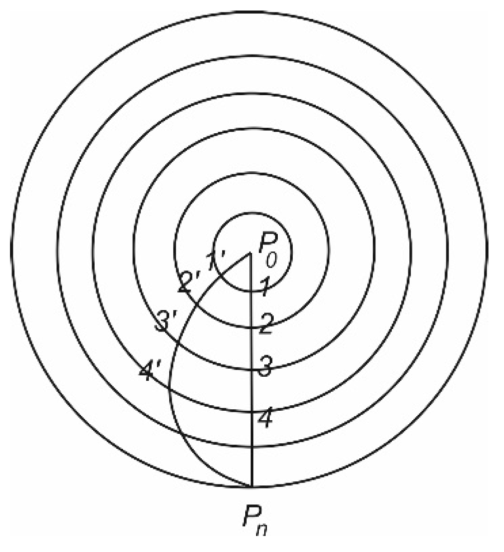
The exception occurs only for P0Pn > π. In that case, the shortest distance is equal to the circumference of the sphere minus P0Pn. Therefore, P0Pn is no longer a relative minimum, since every infinitely close connection between P0 and Pn is shorter on the small circle.
The plane of the greatest circular arc is the common vertical plane not only of the endpoints but also of all the intermediate points, because all radii are normal to the sphere and this plane passes through the centre of the sphere. It is therefore also the plane corresponding to the three infinitely close points of the greatest circular arc, i.e. the oscillating plane at the corresponding point is also a vertical plane. Because of this property of the greatest circular arc, it can also be called a geodesic on the sphere.
To explain this expression, let us imagine that the inhabitants of an arbitrarily curved surface, which is also a level surface, are given the task of drawing a straight line in terms of geodetic practice from point P0 in a given direction.
Then we will first lay a vertical plane from P0 in that direction and place a point P1 on the surface, then lay a vertical plane in P1 through P0 and place a point P2 in it (Figure 1), from P2 in the vertical plane through P1 place a new point P3, etc., where it is tacitly assumed that the adjacent points are so close to each other that there is no noticeable difference between the adjacent vertical planes, so that the three adjacent points lie in a plane, which at this point is the vertical plane of the surface (sphere).
From the above, we can conclude that in the previous sense, a geodetic line, or geodesic, has the described property in relation to its osculating plane.
3. The Orthodrome as the Intersection of a Plane Passing Through the Centre of a Sphere and the Sphere
Let a sphere of radius 1 centred at the origin of the coordinate system be defined by the geographic parameterization
where and are the latitude and longitude respectively, , .
X=cosφcosλ, Y=cosφsinλ, Z=sinφ,
Let us define the orthodrome as the intersection of a plane passing through the centre of a sphere and the sphere. Let us write the equation of the plane passing through the centre of the sphere given by (1):
In this equation, A, B and C are three real numbers. Let us insert the expressions for X, Y and Z from (1) into equation (2). We will obtain the equation of the orthodrome on the sphere in the geographic coordinate system in the form
Let us assume that . After dividing by , equation (3) becomes
If A and B are equal to zero, then equation (4) describes the equator, . Assume that at least one of A and B is not zero and divide (4) by . With the notations
equation (4) can be written in the form
Constants a and can be given a simple geometric interpretation. Namely, it is easy to see that is the longitude of the point where the orthodrome intersects the equator, while a is the cotangent of the angle between the orthodrome and the equator at their intersection. Furthermore, with the assumption , it is easy to obtain that the orthodrome has the highest and lowest point, vertices, whose geographical coordinates are determined by and .
If and , then , i.e. it is the equator.
If , the equation of the orthodrome (6) becomes
and the orthodrome is a meridian circle.
Let the great circle be given by its two points with geographic coordinates and . The unit vectors corresponding to these points are
and the normal vector to the plane to which the orthodrome belongs will be
where
We would arrive at the same result from the condition that three points with coordinates and lie in a plane.
Since the centre of such a circle coincides with the centre of the sphere, and therefore with the centre of the gnomonic projection, the great circle in that projection is mapped into a line. This important property can be used to determine individual points of the orthodrome and to transfer the orthodrome to a map made in any other projection.
4. Orthodrome in the Cartesian Spatial Coordinate System
In the textbook collection of solved problems in vector analysis [10], there is the equation of the orthodrome (which does not include meridian circles):
where , , . The following tasks are solved:
- a)
- Prove that the orthodrome (11) lies on the unit sphere.
- b)
- Prove that the orthodrome (11) lies in the plane passing through the origin, where
- c)
- If a point with geographic coordinates belongs to the great circle, then
- d)
- Show that
- e)
- Show that is the latitude of the point where the orthodrome (11) intersects the equator
- f)
- If and are two points of the orthodrome then
- g)
- Show that a is the cotangent of the angle between the orthodrome and the equator at their intersection.
- h)
- If and are two points of the orthodrome, then it is
- i)
- The angle between the orthodrome and the meridian passing through the point is determined by the relation
- j)
- Show that by appropriately rotating the spatial coordinate system around the origin, the equation of the orthodrome can be transformed into the formwhere and are two unit and mutually perpendicular vectors, .
5. Orthodrome as a Geodesic on a Sphere
Let the orthodrome be a geodesic on the sphere. A geodesic on a surface can be defined in several ways, e.g. it is
- a)
- a curve for which the geodetic curvature at every point is zero
- b)
- a straight line or curve where at every point the vector of its principal normal and the vector of the normal to the surface are collinear
- c)
- a straight line or curve whose binormal is perpendicular to the normal to the surface at every point
- d)
- a straight line or curve whose osculating plane contains the normal to the surface at every point.
Suppose we are looking for a curve on a sphere where at every point the vector of its principal normal and the vector of the normal to the surface are collinear, i.e. the following holds [11]:
It is obvious that there are no straight lines on a sphere, so we will look for such curves on the sphere for which (17) holds. The normal vector of the sphere at any point is equal to the radius vector of that point
If the curve is parameterized by the arc length s, then its normal vector is
If we insert from (18) and from (19) into (17) we get
Let us determine the parameter . Since is the radius vector of a point on a sphere of radius 1, it is obvious that
We differentiate (21) twice:
Since we have assumed that the curve is parameterized by the arc length s, it holds that
so it is
Multiplying (20) by and using (24) we get
This means that the differential equation of the orthodrome is
Equation (26) is a simple second-order differential equation whose solution is
where and are two constant vectors. Since the orthodrome is a curve on the sphere, (21) holds, and from there it follows that
Vectors and determine the plane that passes through the origin of the coordinate system, so we conclude that the orthodrome, as the intersection of a sphere and a plane through its centre, is a great circle on the sphere.
Now, starting from the differential equation (26), we will derive the equation of the orthodrome in the geographic coordinate system. Let a sphere of radius 1 with the centre at the origin of the coordinate system be defined by the geographic parameterization (1). Let us write (1) in vector form
Let the curve on the sphere be parameterized by the arc length s, i.e. let . Let us calculate the vectors
and
Inserting (30) and (31) into the differential equation of the orthodrome (26), we can write it in terms of the components
Since the last equation is a differential equation with only one unknown function , we will solve that equation first. Let us start by lowering the order, i.e., let us denote
and substitute in (34). After the separation of the variables and a little tidying up, we will get
Let us prepare the last equation for integration.
We integrate and get
where K is the constant of integration. From (38) it first follows
and then
From the last relation it follows
By substituting , , we obtain that
which after integration gives
where L is the constant of integration. From (43) it finally follows
if we choose , for . We can also express
which we will need later.
We still need to determine the function . To do this, multiply (32) by , (33) by and add these two equations. We get
where we marked as before , and since , this will be
Inserting the expressions for and into (46), we obtain after minor rearrangements
From there it follows to the sign
Finally we have
where denotes the additive constant. Instead of (50) we can write
or
If we compare (45) with (51) we see that
This is the equation of the orthodrome in the geographic coordinate system. Comparison with (6) gives the relationship between the constants
6. The Orthodrome as a Geodesic on a Sphere and the Clairaut Theorem
The geodetic curvature of the curve on the surface is defined at a particular point using the relation
where is the unit vector of the tangent to the curve, is the unit vector of the principal normal to the curve, and is the unit vector of the normal to the surface [11]. The mixed product can be written in the form
so , if the vectors and are collinear. We covered this in the previous section. However, due to the well-known property of the mixed product that it will not change if the vectors cyclically swap places, we can also write
where we also recognized that the vector product gives the binormal vector . Therefore, we can now say that , if the vectors and are perpendicular. It does not matter whether the two vectors are unit vectors or not. In this sense, we continue further.
Let a sphere of radius 1 with its centre at the origin of the coordinate system be defined by the geographic parameterization (1). Let us write (1) in vector form (29). The normal vector to the sphere will be
where the first partial derivatives are
Let us calculate second partial derivatives
Let be the equation of a curve on a sphere. Then for this curve we can write
and calculate vectors
The osculation plane is determined by the vectors and , so we can write for the binormal vector . The condition that the normal vector to the surface is perpendicular to the binormal vector can be written in the form
and this is identical to the expression
Let us calculate
Inserting it into (64) and assuming we get
Calculation gives
Substituting (67) and (68) into (65), after minor rearrangements we obtain
and then
and finally
i.e.
In geodesy, the last equation is called Clairaut’s theorem of the geodesic [12]. Alexis Claude Clairaut (1713 – 1765) was a French mathematician, astronomer and geophysicist. It is obvious that the value of the constant K must be in the range . The azimuth α is equal to zero when the orthodrome is equal to the meridian circle arc. In general, it will have the smallest value when the radius of the parallel takes the largest value, i.e. at the equator, when , so it holds
The largest value of angle α, i.e. , corresponds to the smallest value of , therefore
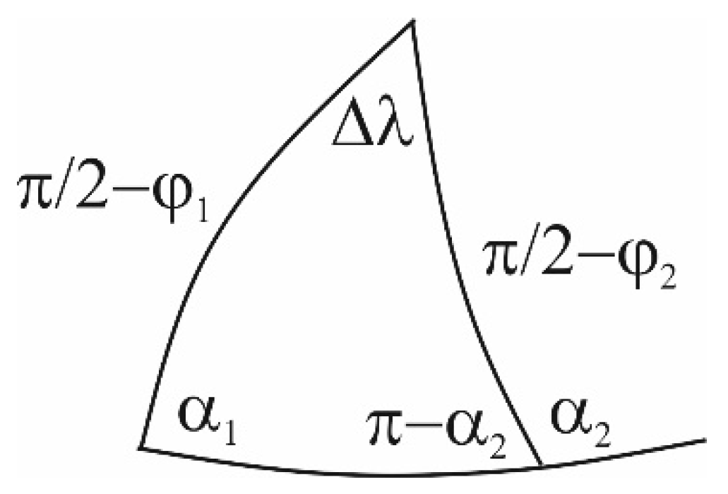
Therefore, the constant K in Clairaut’s theorem is equal to the radius of the northernmost and southernmost parallel that the orthodrome reaches. Clairaut’s theorem for the sphere is identical to the sine theorem in spherical trigonometry. Namely, the sine theorem can be written in the form (Figure 3)
Möhle [13] derived the equation of the geodesic for a surface of revolution in an analogous manner.
Let us also show that (72) is indeed the equation of an orthodrome on the unit sphere. For every curve on the sphere it holds (Figure 2)
If we divide (77) by (76) we get
Clairaut’s equation (72) gives
and then
Accordingly we can write
From there
where denotes the additive constant. From (82) it follows
or (52) or (6).
7. Different Forms of the Clairaut Theorem
The Clairaut theorem can be written in other forms:
Let us show the equivalence of the relations (84)-(87). For every curve on the sphere, (76) and (77) hold (Figure 2). Substituting (77) into (84) we obtain (85). Differentiating (85) with respect to s we obtain
From there
Considering (76) we get (86). If we insert from (77) into (86) we get
and from there (87) follows immediately. Since according to (90) it is
then because of (76) it is
Differentiating (77) with respect to s, we obtain
From the last two equations it follows
and this means that (84) holds. Since (84) follows (85), (85) follows (86), (86) follows (87), and (87) follows (84), it is shown that all four relations (84)-(87) are equivalent.
8. The Orthodrome as a Solution of Differential Equations of a Geodesic
In differential geometry, one can find differential equations for a geodesic on any surface [11,14]:
where , …, are Christoffel notations of the second kind, , , , , and s is the arc length. Elwin Bruno Christoffel (1829-1900) was a German mathematician and physicist. In addition, for any curve parametrized by the arc length,
where , and are first-order Gaussian quantities for the surface.
Let a sphere of radius 1 with the centre at the origin of the coordinate system be defined by the geographic parameterization (1). For this sphere, the first-order Gaussian quantities or the coefficients of the first differential form are equal to
so the first differential form (96) takes the form
The Christoffel notations of the second kind for a sphere have these values:
Substituting (99) into (95) we get
So, geodesics on the sphere will be obtained by solving differential equations (100) and (101) with the help of relation (99). One possibility is to express from relation (99) and include it in (100). This way, we would get a second-order differential equation with an unknown function , which we reduce to a first-order differential equation by lowering the order and then solve it in the usual way. We will describe a slightly shorter procedure.
Let us assume that it is
so we immediately get that the geodesics are meridians, , and then from (100) , , , where and are constants. If we want for , then we should take . If we also want for , we should take .
Let us now assume that
so when we divide (101) by we get
and then
and after integration
where is a constant. After the antilogarithm process (105) becomes
From relation (98) it follows
and then considering (106) it follows
and finally
From (111) it follows
and then
Now we can write according to (106) and (113)
where is the constant of integration. After integration we get
We can obtain a direct relationship between and as follows. From (112) and (113) it follows
while from (116) we get (50) and from there
Finally, from (117) and (119) we obtain (6).
We note another interesting consequence of (101), known as the Clairaut theorem. Note that equation (101) can be written as
From there it follows
and
which is the famous Clairaut theorem.
9. The Orthodrome as a Solution of Differential Equations of a Geodesic on a Surface of Revolution
In differential geometry, differential equations for a geodesic on any surface can be found [11,15]. If it is a surface of revolution, its equation can be written in the form
X=f(φ)cosλ, Y=f(φ)sinλ, Z=gφ.
The differential equations of the geodesic on such a surface read:
where the notation for derivatives was introduced
Since for a sphere defined by geographic parameterization
it is
so the differential equations of geodesics on the sphere (120) and (121) pass into
and these are differential equations (100) and (101) from the previous section, so they can be solved in the same way as they were solved there.
10. The Orthodrome as the Shortest Arc Length of a Curve on a Sphere Connecting Two Points According to Bessel
Let there be two points A and B on a surface. We ask ourselves what is the shortest connection between these points on the surface? For some simpler cases, it is possible to give a necessary condition. Geodesics have the local minimum property: they are curves that are the shortest connections between two points on the surface. In other words, a geodesic is the shortest connection between two sufficiently close points on the surface [11].
The problem of a geodesic as the shortest path between two points on a given surface was addressed by many scientists as early as the 18th century. Bessel provides a concise description of the work of several authors who dealt with this topic, such as Clairaut, Euler, du Séjour, Legendre, and Oriani [9].
Let us take two points A and B on the surface of the ellipsoid of revolution connected by a certain curve. Consider two adjacent points on the curve with latitudes and and longitudes relative to A of and (measured east). Let the distance between them be ds, the azimuth of the line directed towards A be (measured clockwise from north), the radius of the parallel corresponding to the latitude r, and the radius of curvature of the meridian R; then we find
which gives
If we put
then we have
The distance along the curve between two points A and B is therefore
where the integration is from A to B. In order for the curve to be geodesic or the shortest one, the relation between and must be such that the value of the integral is minimal. If we slightly change that relation by replacing with , where is an arbitrary function of that vanishes at the end points (because those points lie on both curves), then the slightly changed length
must be longer than s for each . Let us expand in a Taylor series. We will get
and therefore we have
where we explicitly introduced terms only up to the first order of . For s to be a minimum, it should be
for all . Since this must also hold if is replaced by −, and since we can take so small that the first-order terms are greater than the sum of all other higher-order terms (unless the first-order terms vanish), it follows that the condition for a minimum of s is equal to
Partial integration of the second integral gives
and remembering that vanishes at the endpoints we get
Since the integral should vanish for arbitrary , it must be
or by multiplying by
which, integrating with respect to λ, gives
By substituting we get
which is the well-known characteristic equation of a geodesic. The Bessel derivative shown applies to an ellipsoid of revolution. If we are talking about a unit sphere, then , , so the last equation becomes
where we recognize the Clairaut theorem for the sphere.
11. The Orthodrome as a Solution to the Euler-Lagrange Equation
The brachistochrone is one of many problems in which we want to determine a function y(x) that minimizes or maximizes an integral [16]:
Leonhard Euler was the first to devise a systematic method for solving such problems. Consider, for example, two points, A and B, on a sphere of radius 1 centred at the origin. We want to connect A and B by the shortest, continuously differentiable curve lying on the sphere.
Let the sphere of radius 1 centred at the origin of the coordinate system be defined by the geographic parameterization (1). The first differential form of the mapping (1) is
From there we have
Assume that . Searching for the curve that minimizes the length of the arc between the points and is reduced to finding the function that minimizes the integral
with boundary conditions
Leonhard Euler was the first person to systematize the study of variational problems. His 1744 work [17], Method for Finding Curved Lines Enjoying the Properties of Maximums or Minimums, or the Solution of Isoperimetric Problems in the Widest Sense, is a collection of 100 special problems. The book also contains a general method for solving such problems. Euler abandoned his method in favour of Lagrange’s more elegant “method of variations” after receiving Lagrange’s letter (12 August 1755). Euler also named the subject the calculus of variations in Lagrange’s honour.
This variational derivative has the same role for functionals as the partial derivative has for functions. For a relative (or local) minimum, we expect the derivative to vanish at each point, leaving us with the Euler-Lagrange equation
The Euler-Lagrange equation is only a necessary condition, in the same sense that f’(x) = 0 is a necessary but insufficient condition in mathematical analysis. For general surfaces, the resulting Euler-Lagrange equation is quite complicated [24]. Fortunately, the Euler-Lagrange equation simplifies for some surfaces. The most important special case is the one for surfaces of revolution, i.e., surfaces obtained by rotating a plane curve about an axis. For example, the Euler-Lagrange equation for the unit sphere simplifies to
From there it follows
If we solve the last equation in terms of and integrate, we will get (82) and then (83), (52) or (6).
12. Conclusions
This article provides an overview of the various definitions of the orthodrome, as research has shown that this curve can be approached in about a dozen different ways, which is not common in defining technical terms in geodesy and related fields. Geodesics have been studied and are still studied by many scientists today. A geodesic on a surface is a curve for which the geodetic curvature is zero at every point. Equivalent expressions of this statement are that at every point of this curve the vector of the principal normal is collinear with the normal to the surface, that it is a curve whose binormal at every point is perpendicular to the normal to the surface, and that it is a curve whose osculation plane contains the normal to the surface at every point. In this case, the well-known Clairaut equation of a geodesic naturally appears in geodesy. It is shown that this equation can be written in several different forms. Since corresponding differential equations for geodesics can be found in the literature, but usually without a solution, they are solved in this article. In addition, the orthodrome can also be approached using the calculus of variations, since it is a question of finding the minimum length of an arc.
The article contains a large number of mathematical expressions. To understand the text, basic knowledge of analytical, spherical and differential geometry and the calculus of variations is sufficient. The simplest derivation is using analytical geometry, in which the orthodrome is defined as the intersection of a sphere and a plane passing through its centre. The shortest derivation is using the calculus of variations, but this requires knowledge of the basics of this part of mathematics that is usually not taught in the study of geodesy.
Funding
This research received no external funding.
Data Availability Statement
No new data were created or analyzed in this study. Data sharing is not applicable to this article.
Conflicts of Interest
The author declares no conflicts of interest.
References
- Malinin S. P. Issledovanie kartograficheskih proekcij na ortodromichnost’. Geodezija i kartografija, 1966, No. 6. 61-67.
- Kavrayskiy A. V. O kolichestvennoj ocenke iskazhenija ortodromij v ravnougol’nih proekcijah. Geodezija i kartografija, 1976, No. 1, 61-63.
- Ljusternik L. A. Kratchajshie linii, Varijacionnye zadachi, Gosudarstvennoe izdatel’stvo tehniko-teoreticheskoj literaturi, Moscow, 1965.
- Sigl R. Ebene und sphärische Trigonometrie mit Anwendungen aud Kartographie, Geodäsie und Astronomie. Herbert Wichmann Verlag, Karlsruhe, 1977.
- Krilov V. I. Vivod osnovnih formul sfericheskoj trigonometrii na osnove vektornoj algebri. Izvestija visshih uchebnih zavedenij, Geodezija i aerofotos’emka, 1987, vip. 4, 48-53.
- ret-circle navigation. Available online: https://en.wikipedia.org/wiki/Great-circle_navigation (accessed on 12 November 2024).
- Bessel W. Über die Berechnung der geographischen Längen und Breiten aus geodätischen Vermessungen. Astronomische Nachrichten, Altona, 1826, Band 4, Nr. 86, 241-254. The paper also appears in Abhandlungen von Friedrich Wilhelm Bessel, Vol. 3 (W. Engelmann, Leipzig, 1876). The transcription of Astronomische Nachrichten doi:10.1002/asna.18260041601 has been edited by Charles F. F. Karney and Rodney E. Deakin. The text follows the original; however the mathematical notation has been updated to conform to current conventions. Several errors have been corrected, and the tables have been recomputed. An English translation of this paper with valuable remarks is available at arXiv:0908.1824.
- Helmert F. R. Die mathematischen und physikalischen Theorieen der Höheren Geodäsie, Einleitung und 1. Teil, 1880, Zweiten Auflage, 1962, B. G. Teubner Verlagsgeselschaft. Leipzig.
- Karney Ch. F. F. Geodesics on an ellipsoid of revolution, arXiv:1102.1215v1 [physics.geo-ph] 7 Feb 2011, Link. Available online: http://geographiclib.sourceforge.net/geod.html.
- Lapaine M. Vektorska analiza, Zbirka riješenih zadataka, Geodetski fakultet Sveučilišta u Zagrebu, 2006.
- Lipschutz M. M. Differential Geometry, Schaum’s Outline Series, McGraw Hill Book Company, New York, 1969.
- Clairaut A. C. Determination géometrique de la perpendiculaire a la meridienne tracé par M. Cassini; Avec plusieurs méthodes d’en tirer la grandeur & la figure de laTerre. Mémoire de l’Academie Royal des Sciences de Paris 1733, 406–416 (1735).
- Möhle A. Die Gleichung von Clairaut für geodätische Linien auf Umdrehunsflächen, Differentialgeometrischer Beweis der Gleichung. Zeitschrift für Vermessungswesen, 1938, Heft 4, Band 67, 129-131.
- Christoffel E. B. Allgemeine Theorie der geodätischen Dreiecke, Berlin: Buchdruckeri der Königlichen Akademie der Wissenschaften (G. Vogt), 1869: in Commission bei F. Dümmlers Verlags-Buchhandlung, ETH Library, Rar 15068.
- Carmo M. P. do Differential Geometry of Curves and Surfaces, Prentice-Hall Inc., Englewood Cliffs, New Jersey, 1976.
- Kot M. A First Course in the Calculus of Variations, Americal Mathematical Society, Providence, 2014.
- Euler L. Methodus inveniendi lineas curvas maximi minimive proprietate gaudentes, sive solutio problematis isoperimetrici lattissimo sensu accepti, Opera Omnia, 1744, Series 1, Volume 24, pp.1-308. Available online: https://scholarlycommons.pacific.edu/euler-works/65/ (accessed on 26 January 2025).
Figure 2.
Infinitesimal triangle on the unit sphere. The differential of the arc length of the curve is ds, the differential of the arc length of the meridian is , and the differential of the arc length of the parallel is .
Figure 2.
Infinitesimal triangle on the unit sphere. The differential of the arc length of the curve is ds, the differential of the arc length of the meridian is , and the differential of the arc length of the parallel is .
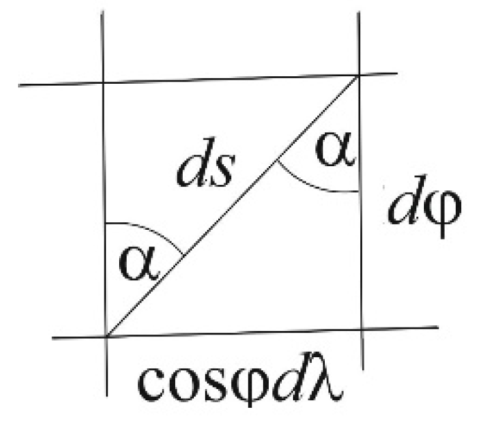
Figure 3.
Polar spherical triangle illustrating the sine and the Clairaut theorems.
Disclaimer/Publisher’s Note: The statements, opinions and data contained in all publications are solely those of the individual author(s) and contributor(s) and not of MDPI and/or the editor(s). MDPI and/or the editor(s) disclaim responsibility for any injury to people or property resulting from any ideas, methods, instructions or products referred to in the content. |
© 2025 by the author. Licensee MDPI, Basel, Switzerland. This article is an open access article distributed under the terms and conditions of the Creative Commons Attribution (CC BY) license (https://creativecommons.org/licenses/by/4.0/).
Copyright: This open access article is published under a Creative Commons CC BY 4.0 license, which permit the free download, distribution, and reuse, provided that the author and preprint are cited in any reuse.


