
Submitted:
10 June 2025
Posted:
12 June 2025
You are already at the latest version
Abstract
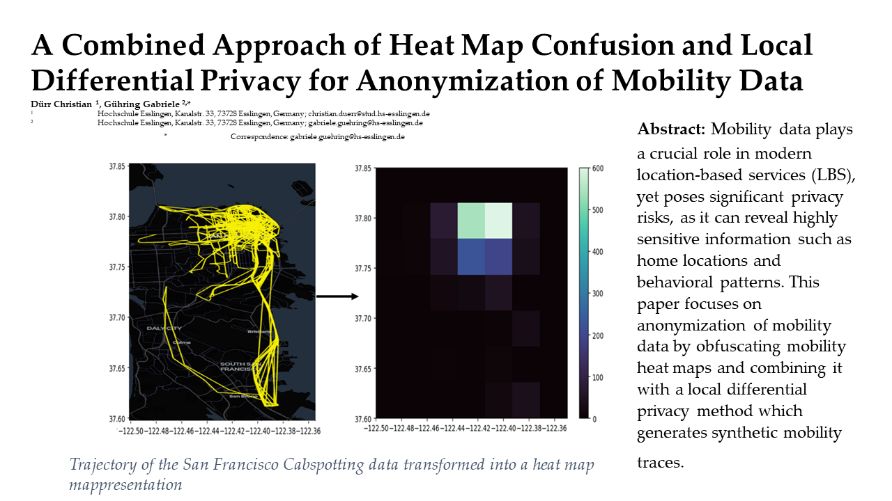
Mobility data plays a crucial role in modern location-based services (LBS), yet poses significant privacy risks, as it can reveal highly sensitive information such as home locations and behavioral patterns. This paper focuses on anonymization of mobility data by obfuscating mobility heat maps and combining it with a local differential privacy method which generates synthetic mobility traces. Using the San Francisco Cabspotting dataset, we compare the effectiveness of the combined approach against reidentification attacks. Our results show that mobility traces treated with both a heat map confusion and local differential privacy are less likely to be re-identified than those anonymized solely with heat map confusion. This two-tiered anonymization process balances the trade-off between privacy and data utility, providing a robust defense against reidentification while preserving data accuracy for practical applications. The findings suggest that the integration of synthetic trace generation with heat map-based obfuscation can significantly enhance the protection of mobility data, offering a stronger solution for privacy-preserving data sharing.
Keywords:
mobility data anonymization
; Heat Map Confusion
; Location Privacy Protection Mechanism
; reidentification attacks
; synthetic mobility traces
1. Introduction
With the rapid advancement of mobile technology, the collection of mobility data has become an integral part of urban planning, transportation systems, and various Location-Based Services (LBS). This data, detailing users' precise movements and locations, offers deep insights but simultaneously poses significant privacy risks [1,2]. Personal information, such as home addresses, workplaces, or even behavioral patterns, can be gathered from mobility data, raising substantial concerns about user privacy [3].
To address these concerns, Location Privacy Protection Mechanisms (LPPMs) have been developed, with the aim to anonymize mobility data while preserving its utility for analysis. Standard LPPMs such as differential privacy [4] and k-anonymity focus on masking individual locations or clustering data points to obfuscate users' identities [2]. However, these techniques often focus on only protecting specific mobility features like the removal of Points of Interest (POIs) to prevent POI-based attacks or the obfuscation of transition probabilities between locations in Markov Chain-based mobility patterns, leaving users vulnerable to in-depth reidentification attacks that leverage comprehensive movement patterns [5].
Heat Map Confusion (HMC) [2,8], which was first suggested by Maouche et. al. [2], is a LPPM that obfuscates mobility traces by transforming them into generalized heat maps, capturing both frequently visited locations and overall movement patterns. HMC protects against reidentification attacks by modifying user profiles to resemble, but not replicate, the profiles of other users. By using these altered heat maps, HMC ensures a balance between maintaining data utility and enhancing privacy protection. The integration of Local Differential Privacy (LDP) [6,7,9] through LDPTrace, as defined in the trajectory synthesis framework [4,7] , enhances the ability of HMC to protect against reidentification attacks.
This paper compares the effectiveness of HMC alone and in combination with LDPTrace (HMC + LDPTrace) against an Aggregate Privacy Attack (AP-Attack) scenario, as defined in section 5. An AP-Attack tries to uncover personal information by analyzing patterns in combined mobility data, like heat maps. To anonymize mobility data via heat maps is a common method explored in the literature, see [10].
While HMC focuses on obfuscating mobility patterns through heat map alterations, LDP adds a layer of differential privacy by introducing controlled randomness, ensuring that individual data points remain unidentifiable even in aggregated datasets. Using the San Francisco Cabspotting dataset, which includes detailed taxi movement records, we evaluate both HMC and HMC plus LDPTrace, assessing their ability to protect user privacy without sacrificing the quality and utility of the data.
This paper provides new insights into how combined anonymization methods can address the increasing challenges of privacy protection in mobility data:
- It utilizes a combined approach using HMC and LDP to address vulnerabilities in mobility data anonymization, which has not been explored together before.
- It integrates LDP through LDPTrace to enhance HMC’s resistance against Aggregate Privacy (AP-Attacks), a novel improvement over using HMC alone.
- The approach emphasizes preserving both individual privacy and utility of aggregate mobility data, achieving a balance not previously demonstrated in comparable methods.
2. Heat Map Confusion
Heat Map Confusion (HMC) [1,2,8] is used to anonymize mobility traces. HMC is an LPPM designed to protect users' mobility data from reidentification attacks by using detailed heat map representations of movement patterns. Unlike standard LPPMs that mainly focus on small-scale mobility data, such as single location points, HMC works with broader mobility features. It transforms user data into heat maps that show frequently visited places and overall movement trends (see Figure 1) as suggested by [2].
Main Principles of HMC
- Heat Map Creation: The first step in the HMC process is to turn a user’s mobility trace . A mobility Trace of length is a sequence of latitude, longitude and timestamp: into a heat map . The heat map creation step involves dividing a specific geographical area into a grid of squares, where each cell represents a location. The intensity of each cell shows how often a specific user has visited that spot (see Figure 1). This approach makes raw GPS data more general, creating a wider view of movement patterns and hiding precise location details.
- Heat Map Alteration: To anonymize the data, HMC changes each user’s heat map by comparing and merging it with the heat map of a similar user from a reference set . This step ensures that the final heat map does not show unique patterns of the original user. To calculate the similarity of two different heat maps, the Topsøe Divergence is used.
The Topsøe Divergence is a metric used to measure the dissimilarity between two heat maps and [2] and [11].
Here, and represent the probabilities at cell (,) in the specific heatmap. The metric combines two terms: the first measures how diverges from , while the second evaluates how diverges from . A value close to zero indicates high similarity between the distributions, whereas larger values mean greater dissimilarity. The Topsøe divergence is asymmetric version of the Kullback-Leibler divergence and has therefore a range between and , see Table 1 and Table 2.
The merging process works step-by-step and starts with an original heat map that needs to be obfuscated. For this process, two additional heat maps are selected from the entirety of known user profiles : , the heat map that is the most similar to , determined by selecting the profile with the lowest Topsøe divergence, and , the heat map that has the highest utility, determined by the most overlapping visited cells, which is defined as Area Coverage [2].
Area Coverage (AC) is a metric used to compare two mobility traces, and , by checking how similar the areas they cover are. This metric is important because it helps to determine how well an anonymized mobility trace keeps the useful patterns of the original one. AC includes three components: precision, recall, and F-score.
The Area Coverage Precision measures how much of the reconstructed trace T′ overlaps with the original trace T.
Here, represents the set of all cells visited in , and is the set of all cells visited in .
The Area Coverage Recall measures the proportion of cells in the original trace T that are preserved in .
Finally, the Area Coverage F-Score combines precision and recall into a single metric. It is computed as the mean of precision and recall as depicted in Equation 4:
ensures that the reconstructed mobility trace achieves both high precision and recall, reflecting a balance between retaining relevant details from the original trace and minimizing unnecessary noise.
The process of modifying the heat map begins by identifying , the most similar heat map according to Topsøe Divergence, and , the heat map with the best overlap in visited areas, i.e. the best Area Coverage F-Score [2]. An area is defined as a single cell of a given heat map , where . is considered visited when there is at least one record in the mobility trace such that . Overlap between two heat maps consists of all cells , which are visited in both heat maps simultaneously.
If and belong to different users, is returned unchanged. In other cases, is iteratively altered by blending it with . In each iteration step, the values in overlapping cells between and are increased, while values in non-overlapping cells are reduced, creating an altered heat map [2]. The strength of this alteration is determined by an obfuscation factor . This process continues until becomes more similar to than to, or the maximum number of iterations is reached. If no suitable solution is found, is used as the final heat map [2].
For example, in a scenario where has high activity in cells and . Heat map has activity in cells and , while heat map shows activity in cells and . The algorithm will iteratively reduce activity in cell and increase it in cell . At the same time, it keeps some overlap in cell to maintain general movement trends. The result is a new heat map that protects privacy but still keeps the overall movement patterns useful for analysis.
- 3.
- Mobility Trace Reconstruction: After the heat map is modified into the obfuscated heat map , the next step is to reconstruct an anonymized mobility trace that corresponds to . The process is described in detail in [2].
Mobility Trace Reconstruction results in the reconstructed mobility trace following the general patterns of movement seen in the original trace , such as frequent visits to certain areas and realistic travel routes [2]. However, the exact details of the original movements are altered to prevent reidentification.
The entire process of HMC is displayed in Figure 2.
HMC is especially effective in protecting against reidentification attacks, such as the AP-Attack, as defined in section 5, which uses combined heat map data to identify users. By changing heat maps to hide specific user patterns, HMC reduces the uniqueness of mobility traces. Thus, it protects up to 87% of users against reidentification, with minimal loss of data utility [2].
3. Local Differential Privacy
To ensure robust privacy protection for mobility data, the concept of ε-Differential Privacy is frequently used. It guarantees that the inclusion or exclusion of any single data entry in a database does not significantly alter the results of queries, thereby protecting individual user information [9]. Formally (see Equation 5), an algorithm satisfies ε-Differential Privacy if for all databases and , differing by at most one element, and any possible outcome of , the following condition holds:
In this formula, represents the privacy budget, which controls the balance between privacy and data utility [9]. A smaller value means stronger privacy guarantees because more noise is added to the data, making it harder to infer individual user details. However, this also reduces the usefulness of the data for analytical purposes. Conversely, a larger offers higher data accuracy but weaker privacy [9]. When applied to mobility data, this balance is particularly critical as even slight inaccuracies can disrupt transportation models or infrastructure planning. Thus, selecting an appropriate ϵ value depends on the specific application and the sensitivity of the data. [6,7,9]
Unlike traditional differential privacy that requires a trusted data curator, LDP ensures privacy by allowing users to perturb their own data before sharing it. This protects individual trajectory data by guaranteeing that even if data is intercepted or analyzed, the original patterns remain private.
In [4], LDPTrace, a concept for -Local Differential Privacy for mobility data is implemented. As HMC, LDPTrace works on a grid of rectangular cells covering the examined area. In order to implement LDPTrace the following steps are performed:
- Feature Extraction: LDPTrace extracts three main features from individual users trajectories and obfuscates them with a privacy budget :
- Intra-trajectory Transitions: The movement between consecutive cells in a grid of a trajectory, capturing local movement behavior.
- Start and End Points: Virtual markers indicating where trajectories begin and terminate, which help in preserving trajectory structures.
- Trajectory Length: With the obfuscated trajectory length of each trajectory a probability distribution of trajectory lengths is determined by a central data curator.
- 2.
- Frequency Estimation: To estimate frequencies for trajectory synthesis, Optimized Unary Encoding (OUE) is used for each of the features extracted. OUE represents each feature as a binary vector of length equaling the maximal value of the feature, where at the index which equals the feature value and zero otherwise. OUE adds noise to binary data to protect privacy before combining the data [3]. As depicted in Equation 6, the probability of a perturbed vector at index i being 1 is defined as:
Here, represents the privacy budget, with smaller values ensuring stronger privacy at the cost of higher noise. This mechanism ensures that reconstructed trajectories retain key statistical properties, such as region transitions and visit frequencies, while safeguarding individual user data.
- 3.
- Adaptive Synthesis Process: The framework builds a probabilistic model using these extracted features, allowing it to generate synthetic trajectories that mimic real movement patterns [12]. The synthesis process is adaptive, meaning it selects transitions and trajectory lengths based on learned distributions without needing exact user data, thus enhancing privacy.
Trajectory synthesis under Local Differential Privacy ensures that user mobility patterns can be anonymized without sacrificing their statistical utility. In [3] a Markov-chain-based model is used to probabilistically synthesize trajectories. In [9] a graph-based model offers the possibility to use more flexible grids. LDPTrace models transitions between regions, as well as the distribution of start and end points, to replicate realistic mobility behavior. By utilizing these probabilistic distributions, LDPTrace preserves the overall structure of the mobility data while effectively anonymizing individual details.
LDPTrace offers several benefits over traditional trajectory anonymization methods:
- Enhanced Privacy Protection: By employing local differential privacy, LDPTrace reduces the risk associated with data aggregation and central storage, ensuring that users' real movement data is not exposed [4].
- Improved Utility: The framework maintains high data utility, as synthetic trajectories generated by LDPTrace closely match real-world movement patterns [4]. This is particularly beneficial for analyses that depend on aggregated mobility trends rather than specific individual behaviors.
- Low Computational Cost: Unlike older methods that rely on intensive computations, such as linear programming or external data integration, LDPTrace simplifies the synthesis process, making it feasible for use on devices with limited resources [4].
- Resistance to Attacks: The method is designed to withstand common location-based attacks, such as reidentification and outlier analysis. By generating trajectories that do not closely mirror any specific user’s data, LDPTrace effectively minimizes vulnerabilities [4].
4. Combination of HMC and LDPTrace
HMC and LDPTrace focus on different aspects of privacy and data utility in mobility data. HMC is designed to protect large-scale mobility patterns by creating and modifying heat maps that represent user traces. It changes these heat maps to look similar to those of other users, which helps protect overall mobility trends and frequently visited areas. This makes HMC effective against attacks that try to identify users based on their general movement behavior. However, it does not focus on protecting individual data points.
On the other hand, LDPTrace uses ε-Differential Privacy to anonymize data at a more detailed level. It adds noise to individual data features and uses probabilistic models to preserve patterns like region transitions and trajectory statistics. This makes LDPTrace better for applications that need detailed data, as it balances privacy and accuracy for each point. While HMC works well for protecting general mobility trends, LDPTrace provides stronger protection for specific data points.
In this paper, we combine HMC with LDP and in particular with LDPTrace. We thus utilize the strength of each method. This is done in the following sequential approach:
- Synthetic Trajectory Generation with LDPTrace: First, LDPTrace creates synthetic mobility traces based on real mobility data from the San Francisco taxi dataset. These synthetic trajectories simulate movement patterns without directly revealing actual user locations. By introducing randomness in location data, LDPTrace makes it harder to link specific movements to real individuals while maintaining patterns that resemble real-world data.
- Heat Map Confusion on Synthetic Data: Once the synthetic trajectories are generated, HMC further anonymizes the data. HMC creates heat maps from these synthetic traces and then alters them by merging similar patterns. This step reduces the likelihood of reidentification based on movement patterns, as individual traces are grouped into less specific patterns. By transforming synthetic data into altered heat maps, this combined approach provides additional protection for individual locations and routes.
5. Aggregate Privacy Attack
An AP-Attack (Aggregate Privacy Attack) [2,8] is a reidentification method that aims to identify users by analyzing their movement patterns as shown in aggregated heat maps. This attack uses frequent locations and movement trends from aggregated heat maps to match individual known mobility profiles [8]. By examining how often a user visits different areas, the AP-Attack compares anonymized data to known patterns. This approach is especially effective on datasets where general movement trends are still visible, as it focuses on commonly visited areas rather than specific locations [2,8].
Figure 3 shows the process of reidentifying users based on their mobility data by carrying out an AP-Attack. The process is divided into two main parts: the training phase and the reidentification phase.
In the training phase [8], mobility data from a set of known users is collected. This data contains their movement traces , which shows where and how these users moved over time. For each user , a mobility profile is created. Each profile abstracts individual movement patterns of the mobility traces into a heat map.
In the reidentification phase [8], a separate set of anonymized data is used. This anonymized data contains movement traces from users whose identities are unknown. For each trace, a profile is created in the same way as in the training phase. These anonymized profiles are then compared to the known user profiles using a distance metric. This metric calculates how similar the two profiles are. In the context of this paper, the Topsøe Divergence is used as a distance metric. The anonymized trace is then matched to the known profile that is most similar.
6. Experimental Evaluation
The Heat Map Confusion (HMC) method and the evaluation of the reidentification rate using AP-Attack are implemented using Python programming language with Visual Studio Code. The following Python libraries are used to conduct the experiments:
NumPy (version 1.26.4): This library is used for numerical operations and handling large datasets, especially for creating and modifying the heat maps.
Pandas (version 2.2.2): Pandas is used for data manipulation, especially for processing the taxi mobility traces and managing time-stamped data.
Matplotlib (version 3.8.4): This library is used to create and visualize heat maps and to plot the results of the experiments.
Scikit-learn (version 1.5.0): It is used for clustering algorithms like KMeans to preprocess the mobility data during the Heat Map Alteration step.
6.1. Dataset
The publicly available San Francisco Cabspotting dataset is used in this study. It includes the GPS traces of 536 taxis collected over a period of 23 days. Each trace includes the latitude, longitude, timestamp, and the occupancy status of a taxi. The San Francisco Cabspotting dataset is a commonly used publicly available dataset. It therefore serves as a benchmark for several anonymization algorithms, see [1,2,4,7,8]. The dataset is processed to convert the raw GPS data into heat maps. All data used in this study can be accessed publicly for replication [12].
To simulate the training and reidentification phases effectively, it is necessary to partition the mobility data sets. The splitting process involves dividing the trajectories of each taxi randomly to ensure variability and avoid bias into a 50 % training and a 50 % reidentification data set.
As in [2] we divide the geographical area into an 8x8 grid of squares of the metro area of San Francisco, each bin roughly 800 meters of height and length. Each cell in the heat map shows how often a single taxi visits a specific location, see Figure 1.
The coordinates used as area are Latitude: 37.60–37.85, Longitude: -122.50–-122.35.
6.2. Evaluation with Aggregate Privacy Attack
To test how well HMC and LDPTrace protect data, we apply an AP-Attack in two steps:
- AP-Attack on unaltered Heat Maps: The AP-Attack is first applied to the original heat maps, which have not been anonymized with HMC. This provides a baseline reidentification rate, showing how easily a taxi can be reidentified without any further anonymization.
- AP-Attack on obfuscated Heat Maps: The AP-Attack is applied to the heat maps after the HMC anonymization process. Comparing the reidentification rates from the original and altered maps shows whether the HMC process is effective. A lower reidentification rate indicates successful anonymization.
In both cases, tests are conducted with synthesized (created with LDPTrace, based on the San Francisco Cabspotting dataset) and non-synthesized trajectories (the original trajectories from the San Francisco Cabspotting dataset). This allows us to compare how well the different approaches perform under varying circumstances.
The results of the AP-Attacks performed on the San Francisco Cabspotting dataset are presented in Table 1 and Table 2 for the non-obfuscated baseline data and the data processed with HMC. In contrast, Table 3 and Table 4 display the outcomes when using synthesized trajectories generated by LDPTrace. While Table 1, Table 2, Table 3 and Table 4 summarize the average values and standard deviations across all trials, Table 5, Table 6, Table 7 and Table 8 in the Appendix provide a detailed breakdown of nine individual trials.
To maintain consistency, randomness is controlled by setting nine pre-defined NumPy np.random seeds, which ensure that the same random trajectories are used across trials. Each scenario is conducted over nine separate trials, ensuring consistent and reliable results by reducing the influence of random variations in the data partitioning process.
The following terms explain the metrics used in the results tables:
- (Non-)Reidentified Total: Refers to the total number of (un-)successful reidentifications.
- (Non-)Reidentified (%): Refers to the percentage of (un-)successful reidentifications.
- Seed: NumPy seed set with np.random. It influences how the data sets are partitioned into train and test data sets.
- Average Distance: The average minimum distance determined by calculating Topsøe Divergence, see Equation 1, over all 536 data sets.
Table 1 provides an overview of the non-obfuscated dataset, summarizing key metrics across all trials. It includes the average reidentification rate (19.2%) and its standard deviation 6.12, along with the corresponding non-reidentification rate (80.8%). The mean Topsøe Divergence is 0.034, and its standard deviation 0.014. These values function as the baseline for comparing the effectiveness of the obfuscation process.
The detailed results as shown in Table 5 exhibit a Reidentified (%) rate ranging from 8.40% to 28.36%. This highlights the significant risk associated with sharing raw mobility data, as nearly one in five mobility traces can be successfully reidentified without any privacy protection measures. The Average Distance measured as a Topsøe Divergence shows some variance with values ranging from 0.02 to 0.07.
In contrast, the HMC-obfuscated dataset, as shown in Table 2 and Table 6, achieves a substantial reduction in reidentification rates. Compared to Table 1, the average reidentification rate decreases from 19.2% to 1.76%, demonstrating the effectiveness of HMC in enhancing privacy protection. The corresponding non-reidentification rate increases from 80.8% in the non-obfuscated dataset to 98.24% in the HMC-obfuscated dataset.
The Reidentified (%) rate in HMC (Table 6) ranges from 0.56% to 2.5%, with an average significantly lower than in the non-obfuscated dataset. The lowest reidentification rate appears in Trial 4 (0.56%), while the highest (2.5%) occurs in Trial 1and Trial 6. The Average Distance (Topsøe Divergence) values for the HMC dataset range from 0.05 to 0.10, which is a bit over the value of the non-obfuscated dataset. This suggests that HMC alone effectively increases anonymity and reduces the likelihood of reidentification.
In contrast, the HMC-obfuscated synthetic dataset, shown in Table 3 and Table 7, achieves an even greater reduction in reidentification rates. Compared to Table 1, the average reidentification rate drops from 19.2% in the non-obfuscated dataset to just 0.15% to 0.33% in the HMC-obfuscated synthetic dataset depending on the used. The non-reidentification rate increases correspondingly from 99.85% to 99.67%, indicating that the combination of HMC and LDPTrace provides strong privacy protection.
The Reidentified (%) rates in these trials range from 0% in multiple trials (e.g., Trial 2, 3, and 6) to a maximum of 0.37% in several trials, depending on the ε value used.
The parameter is called a privacy budget, it controls the trade-off between privacy and data utility. A smaller ε means stronger privacy protection. However, a lower ε might also results in a higher utility metric i.e. Topsøe Divergence. This is because a lower ε introduces more random noise to the data, making individual traces harder to distinguish but also increasing the overall distortion of mobility patterns [4]. Conversely, larger ε values allow for better data utility, but may increase the risk of reidentification.
In this case, the combined approach results in higher Topsøe Divergence values, particularly for ε = 1, where the average distance reaches 0.16 with a standard deviation of 0.016. This demonstrates a strong level of data protection, significantly enhancing privacy. In comparison, higher values of reduce the Topsøe Divergence.
In comparison, the reidentification rate and average distance of mobility traces obfuscated only with LDPTrace (Table 4) is 0.31% and 0.16 for = 1 respectively. This is significantly lower than the reidentification rate of 19.20% and average distance of 0.034 observed in the non-obfuscated dataset (Table 1). However, when both HMC and LDPTrace are applied (Table 3), for = 1 the reidentification rate drops further to 0.19%, and the average distance increases to 0.162, highlighting the enhanced privacy protection achieved by combining both anonymization techniques.
7. Conclusions
The results indicate that in general the higher the level of privacy, the greater the average distance measured with the Topsøe Divergence.
However, the comparison between using HMC alone and combining it with LDPTrace gives several important insights:
- HMC alone is effective at lowering Reidentified (%) rates, with average distances from 0.05 to 0.10, as shown in Table 6. This indicates that HMC can offer privacy protection while keeping data reasonably useful.
- HMC combined with LDPTrace provides stronger privacy, as shown by the lower Reidentified (%) rates between 0% and 0.37% in Table 7, and larger average distances up to 0.20. This demonstrates that the additional application of HMC further strengthens anonymization.
While LDPTrace alone increases Topsøe Divergence nearly tenfold, reflecting its strong anonymization effect, adding HMC does not significantly increase this distance further. Instead, it provides a substantial additional drop in reidentification rates, implying that HMC complements LDPTrace effectively by improving anonymization without further distorting the data.
On the whole, we manage to show that the synthesized trajectories created with the LDPTrace algorithm can be further anonymized and made inaccessible by attacks by adding HMC anonymization.
To enhance the balance between privacy and data utility, future research should focus on:
- Application-specific studies: Analyzing how different data modification levels impact specific applications or use cases, i.e. environmental pollution or traffic simulations
- Including other utility metrics: Creating or utilizing other metrics beyond average distance, such as checking for time-based consistency and the accuracy of points of interest (POI), can offer a clearer view of data usability.
- Experiments with other attacks: To strengthen the robustness of privacy protection methods and ensure comprehensive evaluation, future work should focus on testing additional attack scenarios and analyzing their impact on reidentification rates and data utility. This could include exploring attacks such as outlier detection, POI (Point of Interest)-based attacks, and PIT (Point-in-Time)-based attacks, see [2].
Achieving strong privacy protection while maintaining data utility is crucial for practical applications. The fact that HMC enhances LDPTrace’s anonymization without introducing additional distortion makes this combined approach especially promising.
Author Contributions
Conceptualization, Writing – review & editing, Gühring Gabriele; Software, Writing – original draft, Dürr Christian.
Funding
This research was funded by the German Federal Ministry of Research, Technology and Space (BMFTR), grant number 16KISA046K.
Appendix A

Table 5.
Non-Obfuscated Normal Data Set – Complete.
| Metrics | Trial 1 | Trial 2 | Trial 3 | Trial 4 | Trial 5 | Trial 6 | Trial 7 | Trial 8 | Trial 9 | |
|---|---|---|---|---|---|---|---|---|---|---|
| #Taxi Id | 536 | 536 | 536 | 536 | 536 | 536 | 536 | 536 | 536 | |
| Reidentified Total | 152 | 82 | 141 | 45 | 140 | 83 | 90 | 96 | 97 | |
| Non-Reidentified Total | 384 | 454 | 395 | 491 | 396 | 453 | 446 | 440 | 439 | |
| Reidentified (%) | 28.36 | 15.30 | 26.31 | 8.40 | 26.12 | 15.49 | 16.79 | 17.91 | 18.10 | |
| Non-Reidentified (%) | 71.64 | 84.70 | 73.69 | 91.60 | 73.88 | 84.51 | 83.21 | 82.09 | 81.90 | |
| Seed | 845 | 286 | 742 | 301 | 87 | 123 | 581 | 445 | 4 | |
| ⌀ Topsøe Divergence | 0.02 | 0.03 | 0.03 | 0.07 | 0.03 | 0.03 | 0.04 | 0.03 | 0.03 |
Table 6.
HMC Obfuscated Normal Data Set – Complete.
| Metrics | Trial 1 | Trial 2 | Trial 3 | Trial 4 | Trial 5 | Trial 6 | Trial 7 | Trial 8 | Trial 9 | |
|---|---|---|---|---|---|---|---|---|---|---|
| #Taxi Id | 536 | 536 | 536 | 536 | 536 | 536 | 536 | 536 | 536 | |
| Reidentified Total | 11 | 12 | 10 | 3 | 9 | 11 | 7 | 12 | 5 | |
| Non-Reidentified Total | 525 | 524 | 526 | 533 | 527 | 525 | 529 | 524 | 531 | |
| Reidentified (%) | 2.50 | 2.24 | 1.87 | 0.56 | 1.68 | 2.50 | 1.31 | 2.24 | 0.93 | |
| Non-Reidentified (%) | 97.50 | 97.76 | 98.13 | 99.44 | 98.32 | 97.50 | 98.69 | 97.76 | 99.07 | |
| Seed | 845 | 286 | 742 | 301 | 87 | 123 | 581 | 445 | 4 | |
| ⌀ Topsøe Divergence | 0.08 | 0.05 | 0.10 | 0,09 | 0,08 | 0.06 | 0,07 | 0,05 | 0.05 |
Table 7.
HMC-Obfuscated Synthetic Data Set - Complete.
| Metrics | Trial 1 | Trial 2 | Trial 3 | Trial 4 | Trial 5 | Trial 6 | Trial 7 | Trial 8 | Trial 9 | |||||
|---|---|---|---|---|---|---|---|---|---|---|---|---|---|---|
| #Taxi Id | 536 | 536 | 536 | 536 | 536 | 536 | 536 | 536 | 536 | |||||
|
Reidentified Total |
1 | 1 | 1 | 1 | 2 | 1 | 0 | 1 | 1 | 1 | ||||
| 1.5 | 2 | 2 | 1 | 1 | 2 | 2 | 2 | 2 | 2 | |||||
| 22 | 1 | 0 | 0 | 1 | 1 | 1 | 1 | 1 | 1 | |||||
| Non-Reidentified Total | 1 | 535 | 535 | 535 | 534 | 535 | 536 | 535 | 535 | 535 | ||||
| 1.5 | 534 | 534 | 535 | 535 | 534 | 534 | 534 | 534 | 534 | |||||
| 2 | 535 | 536 | 536 | 535 | 535 | 535 | 535 | 535 | 535 | |||||
| Reidentified (%) | 1 | 0.19 | 0.19 | 0.19 | 0.37 | 0.19 | 0 | 0.19 | 0.19 | 0.19 | ||||
| 1.5 | 0.37 | 0.37 | 0.19 | 0.19 | 0.37 | 0.37 | 0.37 | 0.37 | 0.37 | |||||
| 2 | 0.19 | 0 | 0 | 0.19 | 0.19 | 0.19 | 0.19 | 0.19 | 0.19 | |||||
| Non-Reidentified (%) | 1 | 99.81 | 99.81 | 99.81 | 99.63 | 99.81 | 100 | 99.81 | 99.81 | 99.81 | ||||
| 1.5 | 99.63 | 99.63 | 99.81 | 99.81 | 99.63 | 99.63 | 99.63 | 99.63 | 99.63 | |||||
| 2 | 99.81 | 100 | 100 | 99.81 | 99.81 | 99.81 | 99.81 | 99.81 | 99.81 | |||||
| Seed | 845 | 286 | 742 | 301 | 87 | 123 | 581 | 445 | 4 | |||||
| ⌀ Topsoe Divergence | 1 | 0.15 | 0.15 | 0.16 | 0.2 | 0.16 | 0.15 | 0.17 | 0.16 | 0.16 | ||||
| 1.5 | 0.13 | 0.14 | 0.15 | 0.18 | 0.14 | 0.13 | 0.15 | 0.14 | 0.14 | |||||
| 2 | 0.13 | 0.13 | 0.14 | 0.18 | 0.13 | 0.13 | 0.14 | 0.13 | 0.14 | |||||
Table 8.
Non-Obfuscated Synthetic Data Set - Complete.
| Metrics | Trial 1 | Trial 2 | Trial 3 | Trial 4 | Trial 5 | Trial 6 | Trial 7 | Trial 8 | Trial 9 | |||||
|---|---|---|---|---|---|---|---|---|---|---|---|---|---|---|
| #Taxi Id | 536 | 536 | 536 | 536 | 536 | 536 | 536 | 536 | 536 | |||||
|
Reidentified Total |
1 | 2 | 2 | 1 | 2 | 1 | 2 | 1 | 3 | 1 | ||||
| 1.5 | 2 | 3 | 2 | 2 | 2 | 3 | 3 | 4 | 2 | |||||
| 22 | 1 | 1 | 2 | 1 | 2 | 2 | 1 | 1 | 1 | |||||
| Non-Reidentified Total | 1 | 534 | 534 | 535 | 534 | 535 | 534 | 535 | 533 | 535 | ||||
| 1.5 | 534 | 533 | 534 | 534 | 534 | 533 | 533 | 531 | 534 | |||||
| 2 | 535 | 535 | 534 | 535 | 534 | 534 | 535 | 535 | 535 | |||||
| Reidentified (%) | 1 | 0.37 | 0.37 | 0.19 | 0.37 | 0.19 | 0.37 | 0.19 | 0.56 | 0.19 | ||||
| 1.5 | 0.37 | 0.56 | 0.37 | 0.37 | 0.37 | 0.56 | 0.56 | 0.75 | 0.37 | |||||
| 2 | 0.19 | 0.19 | 0.37 | 0.19 | 0.37 | 0.37 | 0.19 | 0.19 | 0.1 | |||||
| Non-Reidentified (%) | 1 | 99.63 | 99.63 | 99.81 | 99.63 | 99.81 | 99.63 | 99.81 | 99.44 | 99.81 | ||||
| 1.5 | 99.63 | 99.44 | 99.63 | 99.63 | 99.63 | 99.44 | 99.44 | 99.25 | 99.63 | |||||
| 2 | 99.81 | 99.81 | 99.63 | 99.81 | 99.63 | 99.63 | 99.81 | 99.81 | 99.81 | |||||
| Seed | 845 | 286 | 742 | 301 | 87 | 123 | 581 | 445 | 4 | |||||
| ⌀ Topsoe Divergence | 1 | 0.15 | 0.15 | 0.16 | 0.2 | 0.16 | 0.15 | 0.17 | 0.15 | 0.16 | ||||
| 1.5 | 0.13 | 0.13 | 0.14 | 0.18 | 0.14 | 0.13 | 0.15 | 0.14 | 0.14 | |||||
| 2 | 0.12 | 0.13 | 0.14 | 0.18 | 0.13 | 0.13 | 0.14 | 0.13 | 0.14 | |||||
References
- Khalfoun, B.; Maouche, M.; Ben Mokhtar, S.; Bouchenak, S. MooD: MObility Data Privacy as Orphan Disease – Experimentation and Deployment Paper. Proc. ACM/IFIP/USENIX Int. Middleware Conf., 2019, Davis, CA, USA.
- Maouche, M.; Ben Mokhtar, S.; Bouchenak, S. HMC: Robust Privacy Protection of Mobility Data against Multiple Re-Identification Attacks. Proc. ACM Interact. Mob. Wearable Ubiquitous Technol. 2018, 2, 1–25. [Google Scholar] [CrossRef]
- Gatzert, N.; Knorre, S.; Müller-Peters, H.; Wagner, F.; Jost, T. Big Data in der Mobilität: Akteure, Geschäftsmodelle und Nutzenpotenziale für die Welt von morgen. Springer Gabler, Wiesbaden, Deutschland, 2023.
- Du, Y.; Hu, Y.; Zhang, Z.; Fang, Z.; Chen, L.; Zheng, B.; Gao, Y. LDPTrace: Locally Differentially Private Trajectory Synthesis. Proc. VLDB Endow. 2023, 16. [Google Scholar] [CrossRef]
- Xu, F.; Tu, Z.; Li, Y.; Zhang, P.; Fu, X.; Jin, D. Trajectory Recovery from Ash: User Privacy is NOT Preserved in Aggregated Mobility Data. Proc. 26th Int. World Wide Web Conf., 2017, Perth, Australia.
- Buchholz, E.; Abuadbba, A.; Wang, S.; Nepal, S.; Kanhere, S.S. SoK: Can Trajectory Generation Combine Privacy and Utility? Proc. Privacy Enhancing Technologies Symposium, 2024, 3, 75–93. [Google Scholar] [CrossRef]
- Primault, V.; Ben Mokhtar, S.; Lauradoux, C.; Brunie, L. Differentially Private Location Privacy in Practice. Transactions on Data Privacy, 2023, 16.
- Maouche, M.; Ben Mokhtar, S.; Bouchenak, S. AP-Attack: A Novel User Re-identification Attack on Mobility Datasets. Proc. 14th EAI Int. Conf. Mobile and Ubiquitous Systems: Computing, Networking and Services (MobiQuitous 2017), Melbourne, Australia, Nov 2017.
- Walter, P., Efremidis, A., & Gühring, G. Anonymization of Mobility Data and its Meta Information using Local Differential Privacy in Combination with Bidirectional Graphs. IEEE Transactions on Dependable and Secure Computing, preprint 2025.
- Kapp, A., Nuñez von Voigt, S., Mihaljević, H., Tschorsch, F., Towards mobility reports with user-level privacy. Journal of Location Based Services, 2023, 17(2), 95–121. [CrossRef]
- Topsøe, F. Some inequalities for information divergence and related measures of discrimination. In: IEEE Transactions on Information Theory 46.4 (2000), pp. 1602–1609. [CrossRef]
- Abul, O.; Bonchi, F.; Nanni, M. Anonymization of Moving Objects Databases by Clustering and Perturbation. Information Systems, 2010, 35, 884–910.
- Piorkowski, M., Sarafijanovic‐Djukic, N., & Grossglauser, M. (2022). CRAWDAD epfl/mobility. IEEE Dataport. [CrossRef]
Figure 1.
Trajectory of the San Francisco Cabspotting data transformed into a heat map mappresentation [8]. Single data points transformed into a heat map representation [8].
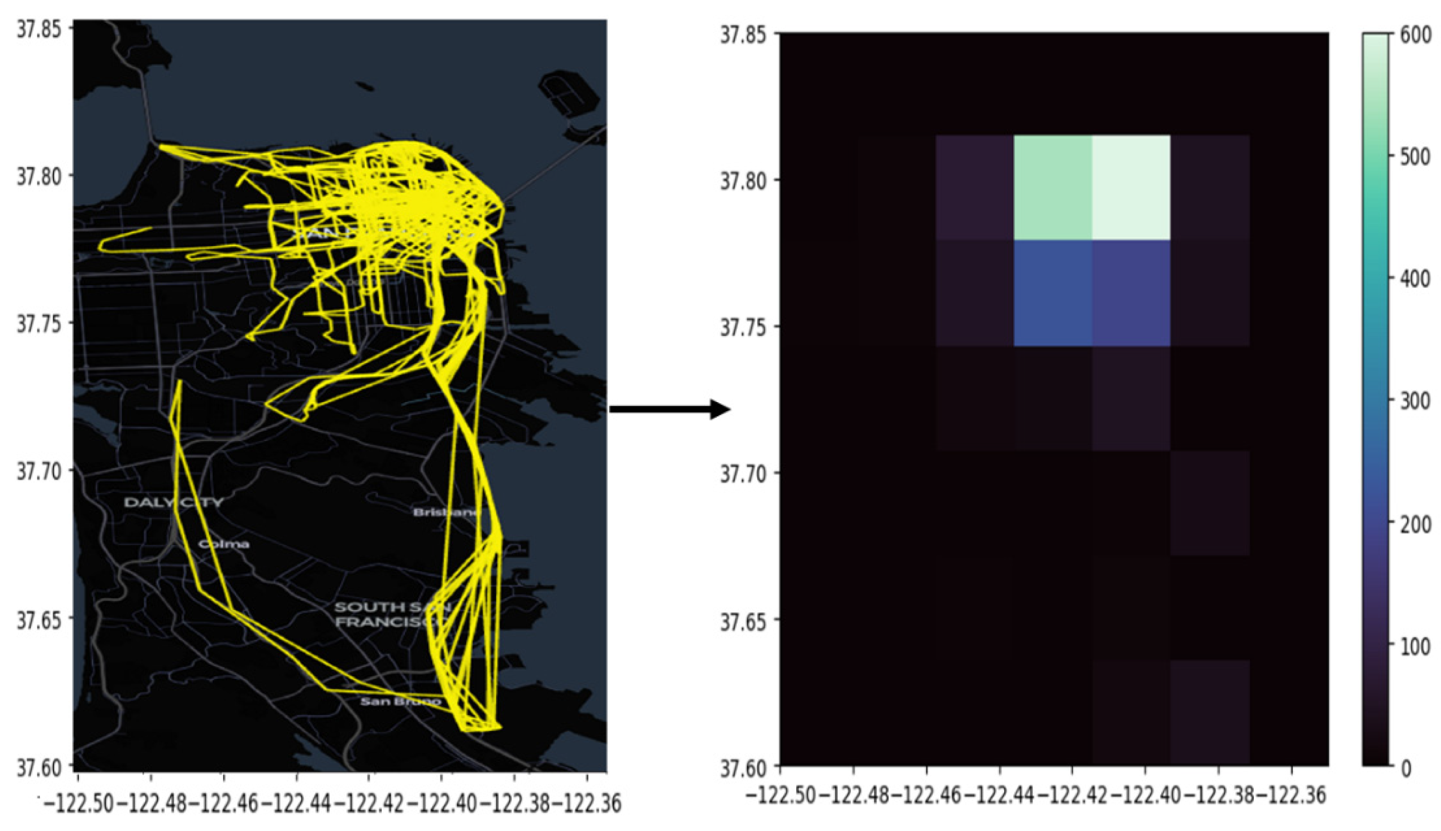
Figure 2.
Heat Map Confusion – Overview [2].
Figure 2.
Heat Map Confusion – Overview [2].
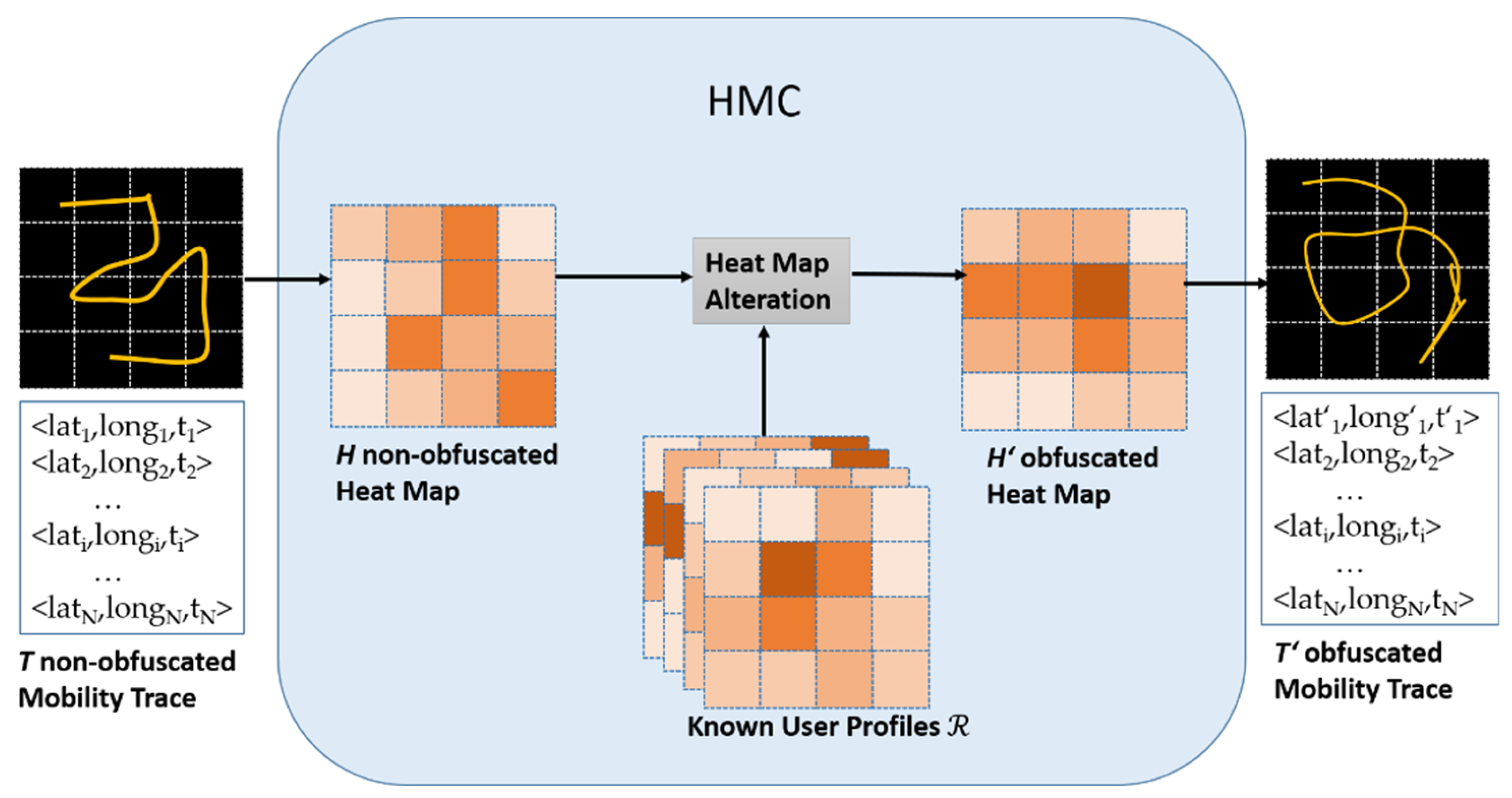
Figure 3.
AP-Attack – Overview [8].
Figure 3.
AP-Attack – Overview [8].
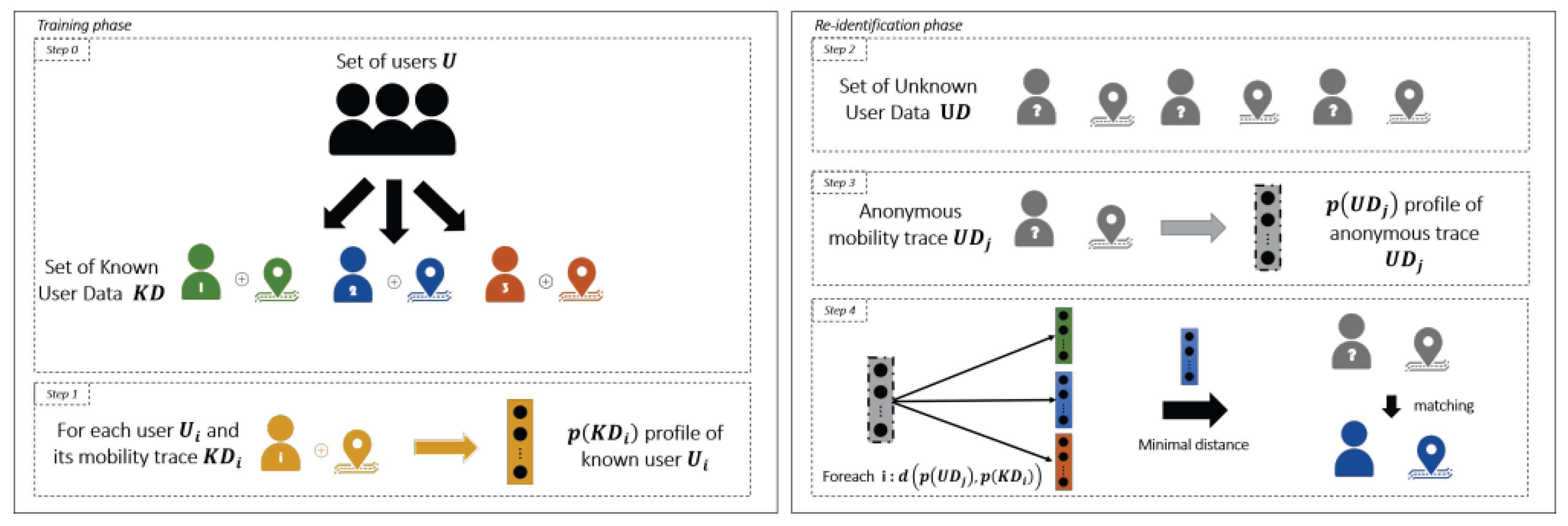
Table 1.
Non-Obfuscated Normal Data Set - Overview.
| Metrics | Mean | Standard Deviation | |
|---|---|---|---|
| Reidentified Total | 103 | 32.784 | |
| Non-Reidentified Total | 433 | ||
| Reidentified (%) | 19.20 | 6.116 | |
| Non-Reidentified (%) | 80.80 | ||
| Average Distance (Topsøe Divergence) |
0.034 | 0.014 |
Table 2.
HMC Obfuscated Normal Data Set – Overview.
| Metrics | Mean | Standard Deviation |
|---|---|---|
| Reidentified Total | 9 | 3.035 |
| Non-Reidentified Total | 527 | |
| Reidentified (%) | 1.76 | 0.659 |
| Non-Reidentified (%) | 98.24 | |
| Average Distance (Topsøe Divergence) |
0.070 | 0.019 |
Table 3.
HMC-Obfuscated Synthetic Data Set - Overview.
| Metrics | Mean | Standard Deviation | |||
|---|---|---|---|---|---|
| Reidentified Total | 1 | 1 | 0.5 | ||
| 1.5 | 1.78 | 0.44 | |||
| 2 | 0.78 | 0.44 | |||
| Non-Reidentified Total | 1 | 535 | 0.5 | ||
| 1.5 | 534.22 | 0.44 | |||
| 2 | 535.22 | 0.44 | |||
| Reidentified (%) | 1 | 0.19 | 0.09 | ||
| 1.5 | 0.33 | 0.08 | |||
| 2 | 0.15 | 0.08 | |||
| Non-Reidentified (%) | 1 | 99.81 | 0.09 | ||
| 1.5 | 99.67 | 0.08 | |||
| 2 | 99.85 | 0.08 | |||
| Average Distance | 1 | 0.162 | 0.016 | ||
| (Topsøe Div.) | 1.5 | 0.144 | 0.015 | ||
| 2 | 0.139 | 0.016 | |||
Table 4.
Non-Obfuscated Synthetic Data Set - Overview.
| Metrics | Mean | Standard Deviation | |||
|---|---|---|---|---|---|
| Reidentified Total | 1 | 1.67 | 0.71 | ||
| 1.5 | 2.56 | 0.73 | |||
| 2 | 1.33 | 0.5 | |||
| Non-Reidentified Total | 1 | 534,33 | 0.71 | ||
| 1.5 | 533.33 | 0.73 | |||
| 2 | 534.67 | 0.5 | |||
| Reidentified (%) | 1 | 0.31 | 0.13 | ||
| 1.5 | 0.48 | 0.14 | |||
| 2 | 0.24 | 0.1 | |||
| Non-Reidentified (%) | 1 | 99.69 | 0.13 | ||
| 1.5 | 99.52 | 0.14 | |||
| 2 | 99.75 | 0.1 | |||
| Average Distance | 1 | 0.161 | 0.016 | ||
| (Topsøe Div.) | 1.5 | 0.142 | 0.016 | ||
| 2 | 0.138 | 0.017 | |||
Disclaimer/Publisher’s Note: The statements, opinions and data contained in all publications are solely those of the individual author(s) and contributor(s) and not of MDPI and/or the editor(s). MDPI and/or the editor(s) disclaim responsibility for any injury to people or property resulting from any ideas, methods, instructions or products referred to in the content. |
© 2025 by the authors. Licensee MDPI, Basel, Switzerland. This article is an open access article distributed under the terms and conditions of the Creative Commons Attribution (CC BY) license (http://creativecommons.org/licenses/by/4.0/).
Copyright: This open access article is published under a Creative Commons CC BY 4.0 license, which permit the free download, distribution, and reuse, provided that the author and preprint are cited in any reuse.


