Submitted:
09 June 2025
Posted:
10 June 2025
You are already at the latest version
Abstract
This study proposes an adaptive refinement method based on feature recognition to achieve rapid solution of the Reynolds equation. Leveraging an isogeometric analysis (IGA) solution framework supporting local refinement, three natural refinement features tailored for solving the Reynolds equation in fluid lubrication including two physical features, pressure value and pressure gradient and an element size feature for discretization are introduced firstly to identify mesh elements. Then a neural network model is trained on feature data to predict element classifications effectively. Finally, this model is integrated into the adaptive refinement solution framework and validated through simulations. Comparative validation was conducted on two distinct Reynolds equation instances, with results demonstrating that the proposed algorithm can effectively evaluate refinement regions globally, avoiding issues such as mesh non-conformity often caused by conventional independent element marking algorithms. The distribution of degrees of freedom is more rational, and the parallel prediction model enhances the speed of the refinement solution.
Keywords:
adaptive refinement
; Reynolds equation
; feature recognition
; neural network
1. Introduction
The Reynolds equation is a fundamental equation in the field of fluid lubrication, derived from the Navier-Stokes equations under specific lubrication conditions[1], and is extensively applied in the analysis and design of lubrication systems. However, fluid lubrication problems typically exhibit unsteady characteristics, such as time-dependent terms[2], dynamic loads[3], and multi-field parameter coupling[4]. Consequently, lubrication analysis or the design of related components often necessitates multiple computations of the Reynolds equation (e.g., for time-varying unsteady problems) or iterative computations (e.g., for multi-field coupling problems). Although current methods for solving the Reynolds equation are relatively mature, including the finite difference method (FDM) [5], finite element method (FEM) [6], finite volume method (FVM) [7], and the increasingly popular IGA[8], the computational efficiency of a single solution process remains a critical concern when addressing repeated solving demands. Improvements in solving efficiency for coupled or time-varying problems can generally be approached from two perspectives: optimizing the solution of the Reynolds equation itself[9] or enhancing the computation of coupled solutions[10]. Clearly, improvements in the former are more universally applicable and can also support the latter.
In Yang, H., various numerical algorithms for solving the Reynolds equation are comprehensively discussed[11], highlighting that the IGA method is particularly well-suited for solving simplified forms of the Reynolds equation. For instance, the normalized computational domain is relatively regular[12], facilitating discretization, while the unrestricted order of IGA basis functions[13] is especially valuable for solving partial differential equations, particularly those with variable coefficients. Consequently, researchers have successfully adapted IGA for the Reynolds equation[14], demonstrating its advantages in this context. In fact, the IGA method closely resembles the finite element method (FEM) in its overall process, and efficiency improvements can similarly be approached from three aspects: discretization quality of the computational domain (meshing), coefficient matrix computation (stiffness matrix assembly), and equation system solving. Among these, the meshing process significantly impacts both solution accuracy and computational time[15]. Generally, mesh size directly correlates with computational time, while mesh layout affects solution accuracy. Therefore, optimizing mesh layout can enhance computational efficiency. In FEM, adaptive refinement techniques[16] control mesh size by allocating denser or higher-quality elements only in regions with larger computational errors, achieving the accuracy of large-scale global refinement with a reduced mesh size. This approach minimizes mesh size while maintaining accuracy, thereby reducing computational time and improving efficiency[17]. IGA can adopt a similar strategy to enhance computational efficiency. Our previous work has explored this approach, yielding promising results.
It is worth noting that most existing adaptive refinement algorithms rely on threshold-based criteria, confining their scope to specific elements or fields[18]. This approach presents two limitations: firstly, thresholds restrict applicability across varying operating conditions, parameter adjustments, or coupling relationships; secondly, effective mesh layout optimization requires both local adjustments to specific elements and global considerations across the computational domain[19]. Compounding these issues, the pronounced nonlinearity of the Reynolds equation[20] renders conventional error estimation algorithms inadequate for accurately capturing errors in complex flows. This stems from a priori and a posteriori error estimation relying on theoretical models[21], which is undermined by continuously varying equation coefficients (e.g., viscosity and pressure), leading to error estimates highly sensitive to convergence point distributions and exhibiting poor stability[22], particularly under significant spatial or temporal variations[23]. To overcome these limitations, this paper proposes classifying mesh elements using natural refinement features, thereby eliminating threshold-related constraints. Furthermore, by employing a neural network model for global-level element recognition and classification within the computational domain, the proposed method enhances mesh layout optimization efficiency while supplanting computationally intensive error calibration techniques.
This paper is structured as follows: Initially, leveraging an IGA framework, three natural refinement features are introduced to classify mesh elements. Subsequently, a neural network model is trained with feature data to predict element categories across the computational domain. This model is then incorporated into an adaptive refinement framework, establishing a feature recognition-based adaptive refinement algorithm. Finally, the algorithm’s effectiveness is validated through simulations and comparative analysis.
2. PHT-Based IGA and Neural Network Feature Recognition
To facilitate understanding of the feature-based refinement process, we briefly outline the IGA refinement approach utilizing PHT and the neural network-driven feature recognition method.
2.1. PHT-Based IGA Refinement
Various methods exist for solving the Reynolds equation, including finite difference methods, finite volume methods, and IGA, each with its own advantages. However, IGA, which combines the high accuracy of finite element methods with the geometric precision of NURBS (Non-Uniform Rational B-Splines)[24], not only efficiently handles complex fluid dynamics problems but also maintains continuity and consistency in the geometric model during mesh generation. In particular, IGA based on PHT splines[25] stands out, as it retains high accuracy and geometric precision while offering local refinement capabilities when solving partial differential equations. When paired with appropriate refinement strategies, the algorithm's efficiency can be further improved. For detailed information on PHT splines, refer to Wen, Z.[26]. The following section briefly introduces the refinement process of PHT splines using a two-dimensional problem as an example.
Figure 1.
PHT Refinement Mesh (a) Initial Mesh Refinement (b) Intra-Element Refinement (c) Adjacent Element Refinement and Deeper-Level Refinement.
Figure 1.
PHT Refinement Mesh (a) Initial Mesh Refinement (b) Intra-Element Refinement (c) Adjacent Element Refinement and Deeper-Level Refinement.
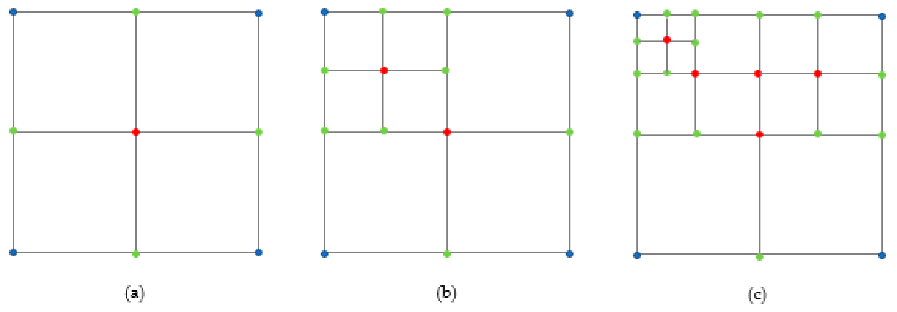
The above figure is an example of local refinement using PHT in IGA, featuring three colored points divided into two categories: interior points and exterior points. Blue points are exterior points, while green and red points are interior points, with interior points further classified as cross points (red points) and T-points (green points). In practice, the PHT method involves inserting a cross at the center of the current element to divide a parent element into four child elements.
The following provides a PHT-based IGA refinement process:
Figure 2.
IGA (PHT) Refinement Steps.

During the refinement process, leveraging the properties of PHT splines, it is only necessary to mark the elements to be refined according to the strategy to reconstruct the parametric domain and complete the refinement process in the physical domain. It should be noted that the IGA method is essentially a parameterized finite element approach, and the PHT-based IGA method by default maps the physical domain to .
2.2. Neural Network-Based Feature Recognition
From the preceding refinement process, it is evident that an appropriate element marking algorithm is critical for optimizing mesh layout. Numerous existing methods enable element marking for region recognition or local refinement[27]. However, these methods often exhibit low efficiency and lack a global perspective, making it challenging to achieve effective adaptability in complex geometric and physical problems. Moreover, they typically permit adjustments only within confined regions, failing to respond effectively to large-scale variations, particularly in handling complex variable-coefficient problems[28], where comprehensive optimization is often unattainable. Most critically, the majority of these algorithms rely on threshold-based specific refinement rules, which impose significant limitations on their applicability.
To address these limitations, employing feature recognition to identify elements for refinement provides an effective solution. Feature recognition methods overcome the constraints of local computation by analyzing key attributes or patterns in data to perform pattern classification and prediction. Currently, mainstream feature recognition methods, represented by machine learning[29], involve algorithms that learn patterns from data to make predictions or decisions. Unlike traditional threshold-based algorithms, machine learning does not rely on explicitly defined rules but adapts models by extracting features and patterns from data. Among various machine learning approaches, neural networks[30] are a particularly popular method. This study employs neural networks for feature recognition, utilizing supervised learning, although other machine learning methods are also applicable.
3. Adaptive Refinement Algorithm Based on Neural Network Feature Recognition
To effectively recognize elements for refinement and achieve the refinement process, this study builds on prior research by first proposing three natural refinement features for solving the Reynolds equation in fluid lubrication: pressure values and pressure gradients as physical characteristics, and element scale features for discrete representation. After extracting these element features, traditional sorting and computational classification are performed on each mesh element, assigning refinement labels based on specific refinement criteria. Subsequently, a neural network model is trained using the existing feature data and corresponding labels, enabling accurate classification and prediction of all mesh elements in the current discrete solution domain. Finally, this model is integrated into an adaptive refinement framework.
This approach considers both local and global perspectives: locally, it calculates feature information, such as physical properties of sampling points within each element and element scale representations (e.g., parametric element area); globally, it defines labels for each element through data processing and classification criteria, marking elements and defining refinement based on label classification. This feature-based refinement approach circumvents threshold constraints, while the introduction of neural networks replaces cumbersome iterative sorting computations, enhancing refinement efficiency and robustness.
3.1. Definition of Element Feature Information
To effectively align with the natural characteristics of lubrication problems, this study adopts physical characteristics (e.g., pressure and pressure gradients) and geometric features (e.g., element size) as evaluation criteria for marking refinement regions. These physical quantities not only possess clear physical significance but also intuitively reflect the impact of different regions on the solution results[31]. Through feature recognition[32], the refinement process extends beyond local optimization, enabling rational judgments based on physical features across the global domain.
The feature information in this study is categorized into physical features and geometric features. Physical feature information, including pressure and pressure gradients, reflects the physical properties of sampling points within each element. Geometric feature information, represented by the absolute size of elements, pertains to regional information.
Considering the correlation between element size and physical information, this study integrates physical and geometric information to propose the concept of relative element scale, aiding in the global assessment of elements.
In summary, the four types of element feature information are shown in the table below.

Table 1.
Element feature information.
| Parameter | Component structure | Definition |
| Pressure | ||
| Pressure gradient | ||
| Element absolute scale | ||
| Element relative scale |
Here, represents the number of Gauss quadrature points.
When extracting feature information, the method of selecting Gauss quadrature points is used to arrange sampling points within the element. In IGA, the numerical solution of the physical field to be solved (Taking the two-dimensional Reynolds equation as an example) at any parametric point position can be expressed as:
Here, represents the spline basis function, and denotes the solution coefficient corresponding to the basis function. are parametric coordinates obtained after geometric mapping of the physical domain. Furthermore, the pressure gradient can be calculated using the following expression.
The pressure gradients in the x-direction (u-direction) and y-direction (v-direction) can be expressed as:
Here, denotes the physical domain,, and represents the derivative vector of the basis function, directly computed from the spline function definition. Similarly, is a 2×2 Jacobian matrix:
Specifically, the Jacobian matrix becomes an identity matrix I in the mapping from physical space to parametric space after PHT discretization, primarily because the derivation of the Reynolds equation involves a regularization of the solution domain that produces a normalization-like effect.
For the geometric feature information , this paper uses the parametric element area, which can be calculated from the coordinates of the element’s four vertices.
The relative scale integrates geometric and physical feature information by multiplying the element pressure value by the element’s absolute scale. Here, the element pressure value , representing the pressure integral over the element domain, can be expressed as:
Here, and represent the pressure value and integration weight calculated at the internal integration points of the element, respectively, while denotes the Jacobian determinant corresponding to the Gaussian integration points, after mapping, it becomes an identity matrix, and the determinant has a value of 1. Assuming all elements adopt the same sampling rule, can be regarded as a constant coefficient, identical for all elements.
approximates the pressure integral of the physical domain, representing the total pressure contribution of the element, which is influenced by the element area . Therefore, the concept of relative scale () is proposed to represent the pressure contribution of the element area.
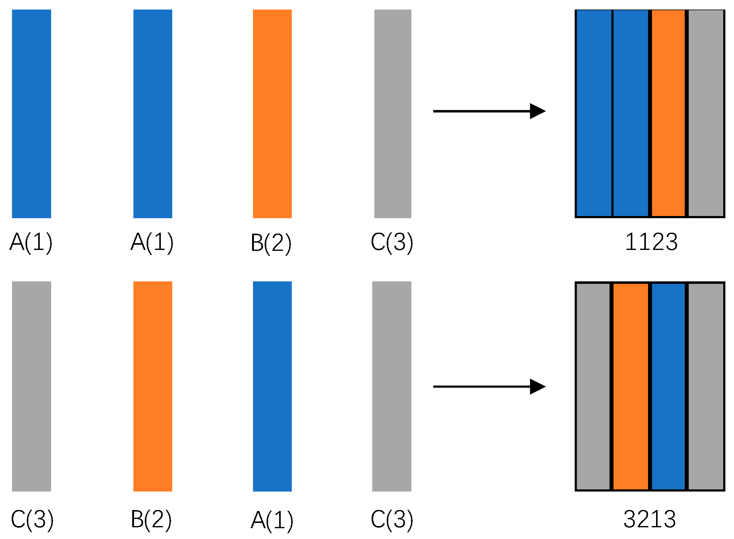
As shown in Figure 3, under the same solution distribution, the physical and geometric features of Element 1 remain unchanged across both discretization scenarios. However, in Scenario 2, the refinement features of Element 1 become more pronounced. This paper enhances the refinement features of Element 1 in Scenario 2 by introducing the element pressure value into the absolute scale to construct a relative scale.
The element feature information can be organized into a set of element feature vectors as shown in Equation (6), providing a basis for subsequent element classification and foundational data for neural network training.
In the equation, denotes the element index.
3.2. Refinement Method Based on Feature Information
This section primarily introduces the process of defining labels for each feature of elements based on element feature data, marking elements for refinement according to a unified refinement classification criterion, and thereby achieving adaptive refinement. Furthermore, a neural network is introduced to perform learning and training on the existing element data and labels, enabling the classification and recognition of element refinement features.
3.2.1 Defining labels for feature information
, , and belong to different data types and exhibit significant differences in magnitude; therefore, they should be standardized[33] separately by category before label definition. Within , and are also standardized individually due to directional differences. The absolute scale is obtained from the mapped parametric coordinates and does not require further standardization. This paper adopts the Z-score standardization method, although other methods may also be applied. The general expression for Z-score is:
In Equation (7), represents the standardized value, is the raw data value, is the mean of the raw data, and is the standard deviation of the raw data. After standardization, the Z-scores for most data points fall within the range of [-3, 3].
After processing the feature information, the element feature vector can be obtained.
It should be particularly noted that the pressure and pressure gradient in the feature information are multidimensional data, whereas the scale information is one-dimensional data. To ensure consistency of standards and enhance the generalization performance of subsequent neural network training, the pressure and pressure gradient data are transformed into one-dimensional data using a method similar to Equation (5), and a new gradient magnitude is introduced as follows:
However, Z-score normalization assumes that the data distribution is approximately normal and only performs linear scaling of relative differences between features, which cannot effectively amplify the differences of certain key features, particularly when the data distribution is asymmetric or contains extreme values. Therefore, before applying Z-score normalization, a nonlinear piecewise transformation based on the median is employed here to preprocess the one-dimensional pressure and pressure gradient data, enhancing their differences and facilitating feature recognition.
Equation (8) represents the basic formula for the nonlinear piecewise transformation based on the median, where is the transformed value, is the original data, and is the median of the data.
After undergoing nonlinear piecewise transformation based on the median and standardization, the feature information of the element is used to obtain the element feature vector for classification. The elements are classified based on three aspects: pressure, pressure gradient, and element scale. First, labels are assigned based on the three types of element features—pressure, pressure gradient, absolute scale, and relative scale. Accordingly, the labels are divided into four categories, which must reflect the characteristic properties of the elements. In brief, larger feature values should correspond to larger label values, while smaller feature values should correspond to smaller label values. To this end, the features need to be classified first. However, the pressure and pressure gradient of an element are random and may exhibit extreme or minimal values, making accurate classification challenging. Dividing them into only "large" and "small" categories is insufficient to fully characterize the features, while dividing them into too many categories, although improving precision, significantly increases workload and may lead to classification redundancy. In contrast, the scale features of the element are easier to define: the absolute scale exhibits regularity, and through refinement, the absolute scale of sub-elements will not exceed that of the parent element; the relative scale implicitly reflects the pressure characteristics of the element, aiding in highlighting pressure features. Therefore, considering the above factors comprehensively, each type of feature is divided into three categories.
This study employs a hierarchical agglomerative clustering method. The Cityblock metric is used as the similarity measure between data points, and the Complete linkage criterion is applied as the inter-cluster connection rule. The dendrogram is divided into three clusters (K=3), and the cluster labels are remapped to 1 (small), 2 (medium), and 3 (large) based on the ascending order of cluster means to reflect the relative magnitude of pressure values. Compared to standard statistical methods (e.g., quantile partitioning), this approach offers greater robustness in handling skewed distributions and outliers, enabling more accurate highlighting of differences in key features.
Due to the binary refinement used in PHT-based IGA elements, the scale relationship between sub-elements and the parent element is 1/4^n, and as shown in Figure 2, the method maps the physical domain to the parametric domain. Therefore, the absolute scale node values of the subdivided elements are fixed values (0.0625, 0.015625), allowing the absolute scale to be directly divided into three categories without requiring the aforementioned clustering method for classification and label definition.
Ultimately, through the above methods, labels corresponding to the four types of feature information of the element can be obtained. These four labels are combined, as shown in Figure 4, to form a four-digit label, which serves as the final feature label for the element.
Figure 6.
Examples of Final Element Feature Labels.
3.2.2. Element Type Definition and Refinement Criteria
Once the feature labels of the element are determined, the elements are classified based on these labels, and those requiring further refinement are explicitly identified to provide a basis for refinement recognition in the neural network. During the classification process, attention must be paid not only to the final feature labels of the elements but also to a comprehensive evaluation incorporating refinement criteria to ensure the accuracy of classification and the rationality of refinement. The core principle of refinement prioritizes scale, with pressure and pressure gradient as supplementary factors. The refinement criteria are as follows:
First, when the absolute scale label of an element is 1 (or 3), regardless of the values of other feature labels, the element must not be subdivided (or must be subdivided). When the absolute scale label is 2, the refinement decision is no longer determined solely by scale but is supplemented by the collective strength of the feature labels. When two or more feature labels or the final label have a value of 3 (i.e., at the upper limit of feature intensity), the element is considered to exhibit high nonlinearity or significant gradient changes across multiple dimensions, indicating pronounced non-uniformity and instability, and thus a high necessity for refinement. Therefore, under the condition of S=2, if the number of “3” labels among the other feature labels is greater than or equal to 2, the element is deemed to require refinement (refinement state m=1); otherwise, it is not subdivided (refinement state m=0).
The classification table is summarized as follows:
Table 2.
Mesh Element Classification.
| () | Final Label (L) | Category (F) | Refinement State (m) | |||
| 3 | 1(2,3) | 1(2,3) | 1(2,3) | 3111(……) | 1 | 1 |
| 1 | 1(2,3) | 1(2,3) | 1(2,3) | 1111(……) | 2 | 0 |
| 2 | 2(3) | 2(3) | 2(3) | 2222(……) | 3 | 1 |
| 2 | 1 | 1(2) | 1(2) | 2111(……) | 4 | 0 |
| 2 | 3 | 1 | 1 | 2311 | 5 | 0 |
| 2 | 3 | 2 | 1 | 2321 | 6 | 1 |
| 2 | 3 | 1 | 2 | 2312 | 7 | 1 |
| 2 | 2 | 1 | 1 | 2211 | 8 | 0 |
| 2 | 2 | 2 | 1 | 2221 | 9 | 0 |
| 2 | 2 | 1 | 2 | 2212 | 10 | 0 |
| 2 | 1 | 3 | 1 | 2131 | 11 | 0 |
| 2 | 1 | 3 | 2 | 2132 | 12 | 1 |
| 2 | 1 | 3 | 3 | 2133 | 13 | 1 |
| 2 | 2 | 1 | 1 | 2211 | 14 | 0 |
| 2 | 2 | 1 | 2 | 2212 | 15 | 0 |
| 2 | 2 | 1 | 3 | 2213 | 16 | 1 |
Ultimately, all elements are classified into 16 categories, with corresponding refinement results for each category (0 indicating no refinement, 1 indicating refinement). The number of categories can be expanded or adjusted as needed. The entire framework for defining labels and classification is structured as shown in the figure below:
Figure 5.
Flowchart for Defining Element Labels and Classification.
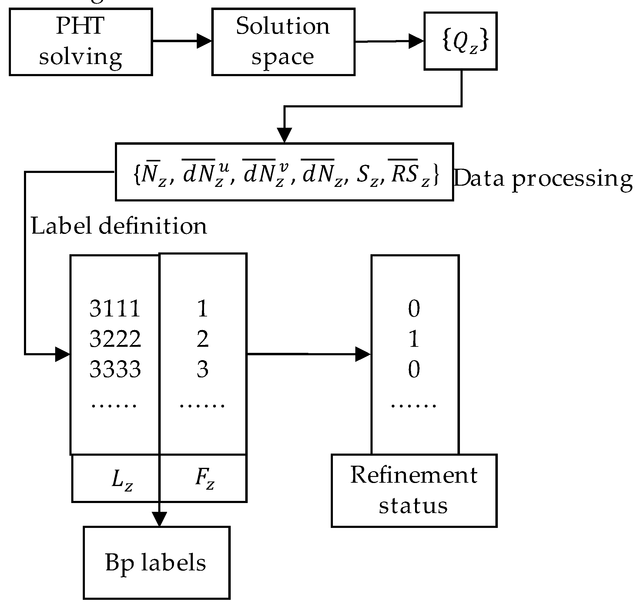
The current solution space is computed using the PHT method, followed by the extraction of feature information for element points and overall element feature information using Gaussian quadrature point techniques. These feature data are then integrated into a set of element feature vectors , which undergo standardization and other processing to generate an optimized group of element feature vectors. Finally, feature labels are defined, and element categories, feature labels, and refinement decisions are determined based on specific refinement criteria. Thus, a feature-based refinement method is fully established.
3.3. Parameter Optimization for Nonlinear Transformation and Clustering Methods
In the aforementioned process, the selection of nonlinear transformation and clustering methods directly impacts the effectiveness of element classification and refinement. Therefore, their specific selection requires systematic analysis and validation. The following elaborates on the methodology and scientific basis for the selection to further demonstrate its rationality.
First, using the hydrostatic sliding bearing model data as an example, the hierarchical clustering parameters are fixed as 'ward' and 'euclidean,' and different nonlinear transformation methods are employed for analysis and validation.
Table 3.
Parameter Settings for Nonlinear Transformation and Hierarchical Clustering.
| Simulation Group | Nonlinear Transformation Method | Hierarchical Clustering Method | Hierarchical Clustering Distance Metric |
| 1 | Median-Based Nonlinear Piecewise Transformation | Ward | Euclidean |
| 2 | Atan-Based Nonlinear Transformation | Ward | Euclidean |
| 3 | Sinh-Based Nonlinear Transformation | Ward | Euclidean |
Figure 6.
The Effect of Three Nonlinear Transformation Methods on the S Value
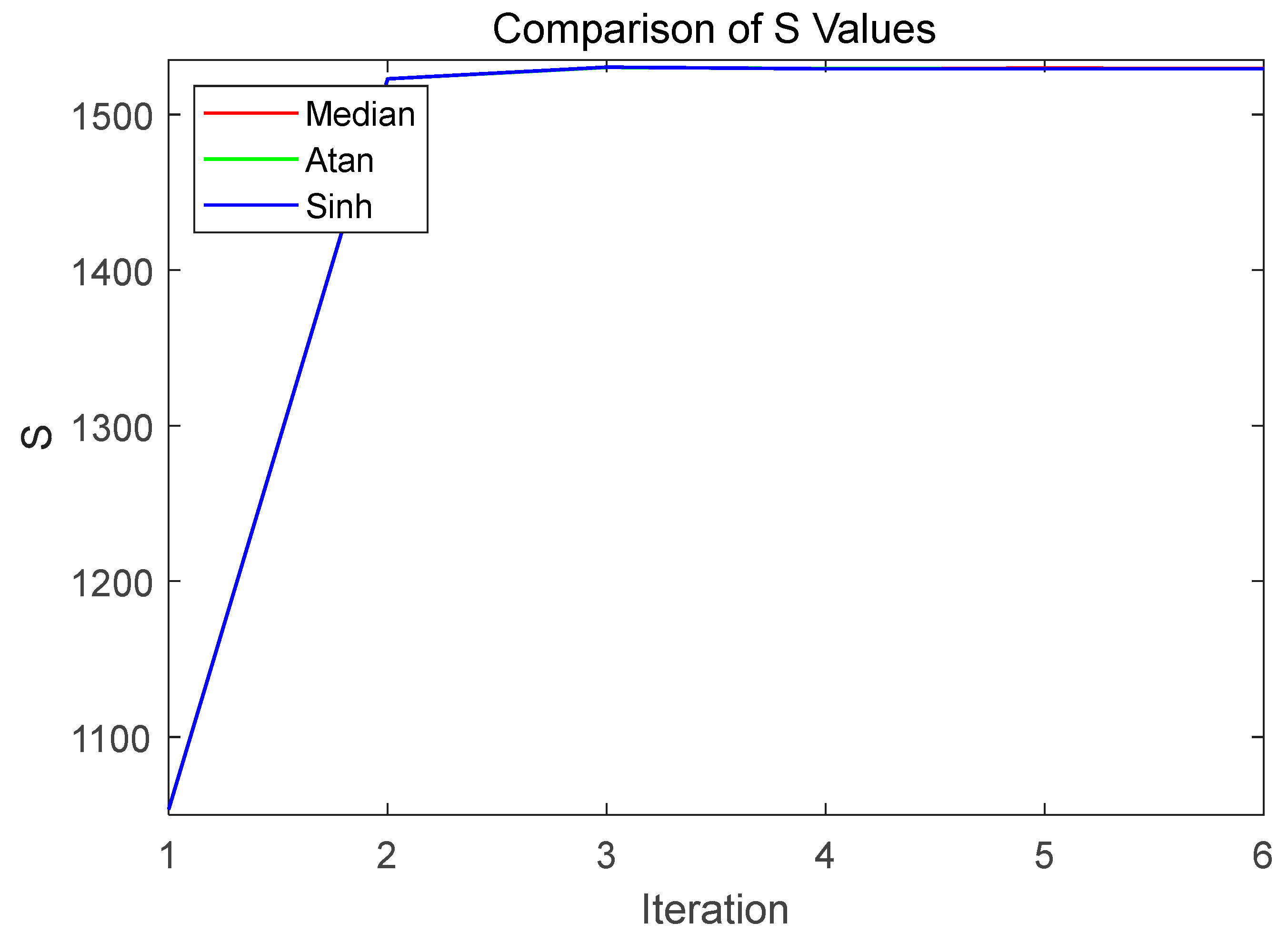
Figure 7.
The Effect of Three Nonlinear Transformation Methods on the DOFS Value
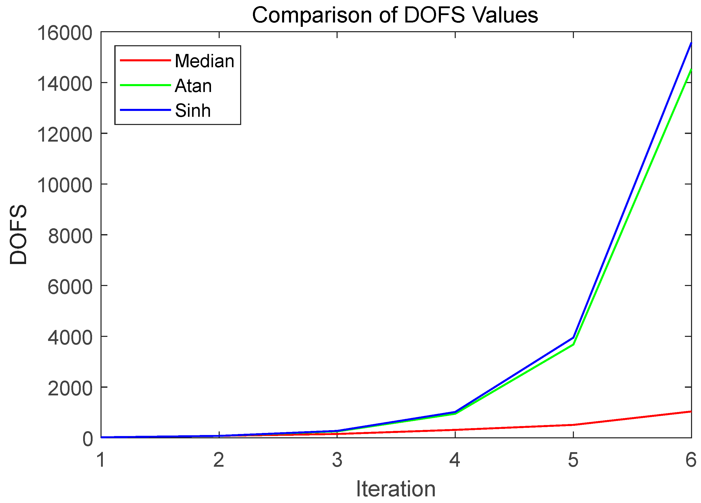
Figure 8.
Iterative Results of Mesh Refinement for Three Nonlinear Transformation Methods.
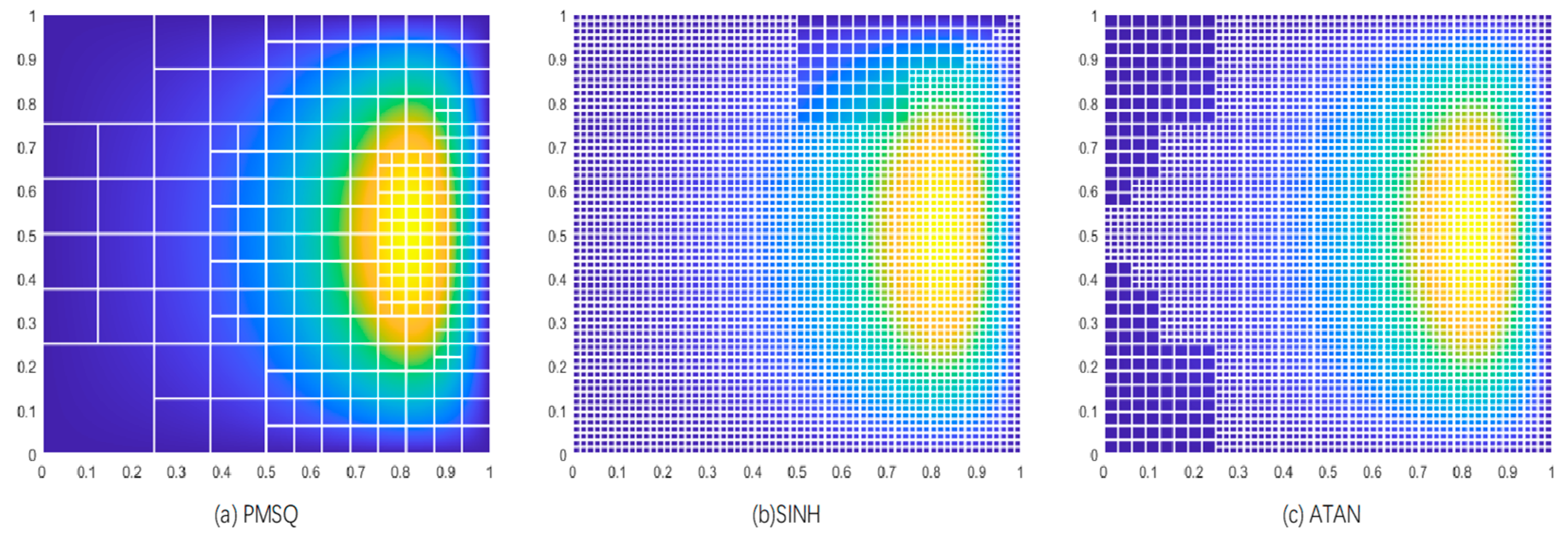
From the first two comparison figures, it is evident that the three methods (Median or PMSQ, ATAN, and SINH) exhibit similar performance in approaching the optimal pressure solution, but they differ significantly in the number of degrees of freedom used. The nonlinear piecewise transformation method based on the median achieves the optimal solution with fewer degrees of freedom, demonstrating higher efficiency and resource utilization. In contrast, while the ATAN and SINH methods can also approach the optimal solution, they require more degrees of freedom, with SINH showing a sharp increase in degrees of freedom in the later stages. The third figure compares the iterative results of mesh refinement, clearly indicating that the ATAN and SINH methods lead to excessive mesh refinement, failing to effectively target critical elements for refined processing. This results in significant resource waste and reduced refinement efficiency. In comparison, the PMSQ (Piecewise Median Square) method prioritizes the refinement of critical elements, with well-defined element hierarchies and high resource utilization efficiency. This suggests that the nonlinear piecewise transformation method based on the median offers superior performance in the refinement process, thereby identifying it as the optimal nonlinear transformation method.
Building on this nonlinear transformation method, fixed hierarchical clustering parameters are no longer used. Instead, different hierarchical clustering parameters are explored to investigate their impact on clustering performance while maintaining consistent cluster settings. By comparing performance metrics under different clustering methods and distance measures, the superiority of the method can be more comprehensively evaluated, ensuring the robustness and adaptability of the results.
Table 4.
Settings of Different Hierarchical Clustering Parameters.
| Simulation Group | Nonlinear Transformation Method | Hierarchical Clustering Method | Hierarchical Clustering Distance Metric |
| 4 | Median-Based Nonlinear Piecewise Transformation | Ward | Euclidean |
| 5 | Median-Based Nonlinear Piecewise Transformation | Complete | Euclidean |
| 6 | Median-Based Nonlinear Piecewise Transformation | Ward | Cityblock |
| 7 | Median-Based Nonlinear Piecewise Transformation | Complete | Cityblock |
Figure 9.
The Effect of Different Hierarchical Clustering Parameters on the S Value
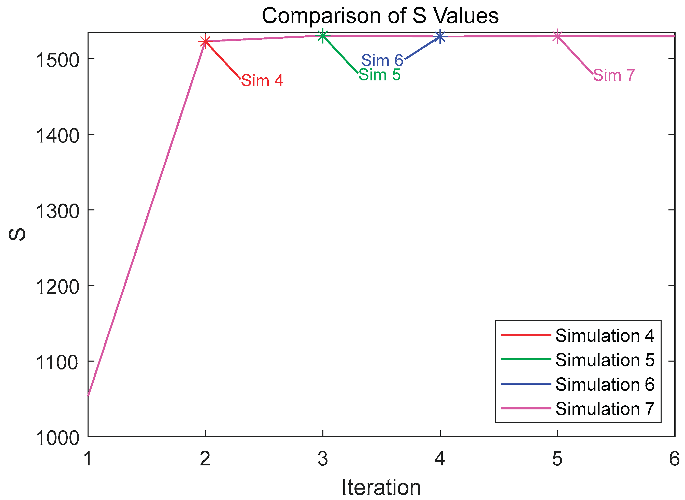
Figure 10.
The Effect of Different Hierarchical Clustering Parameters on the DOFS Value
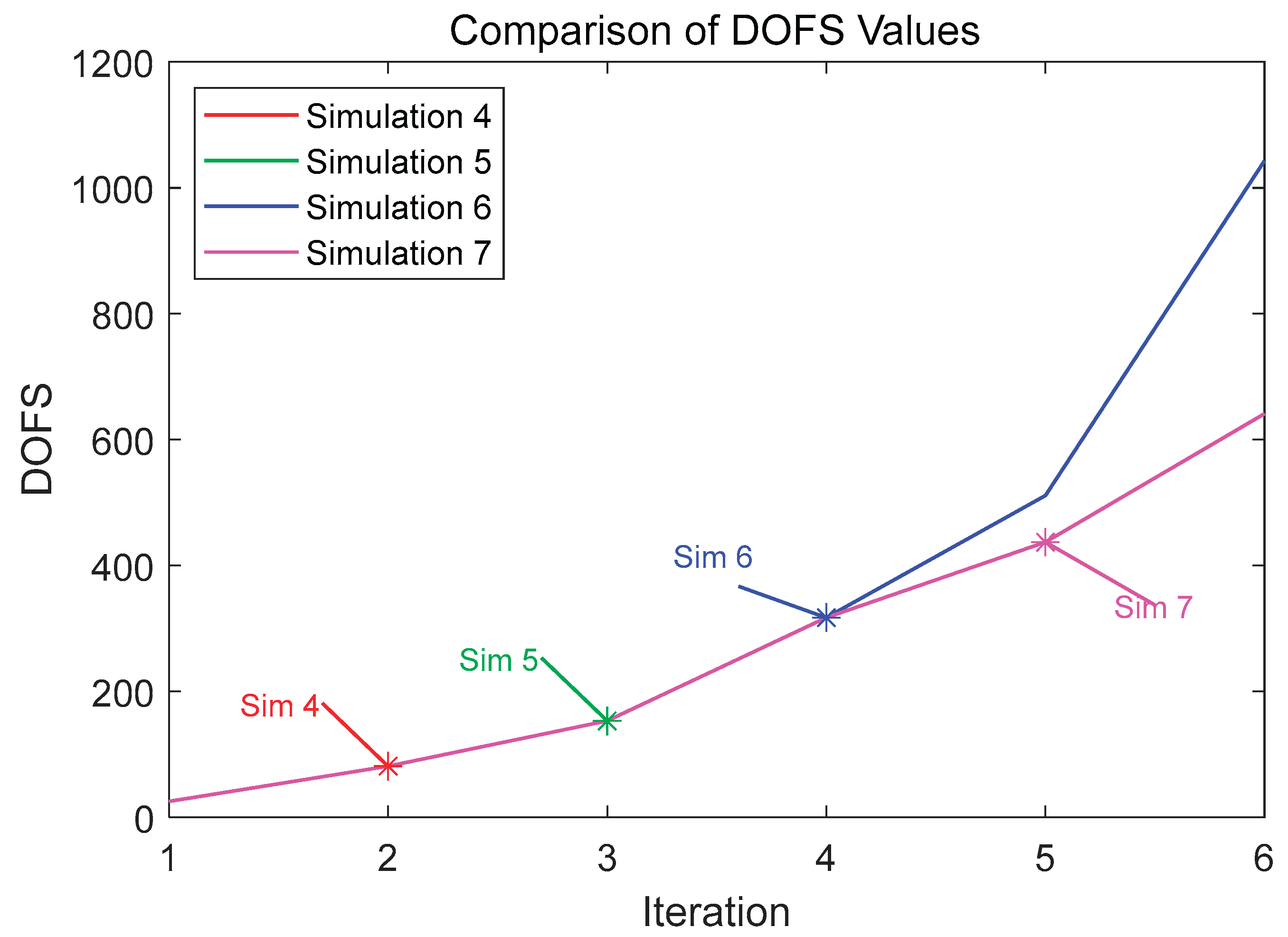
Figure 11.
Iterative Results of Mesh Refinement for Four Simulation Groups.
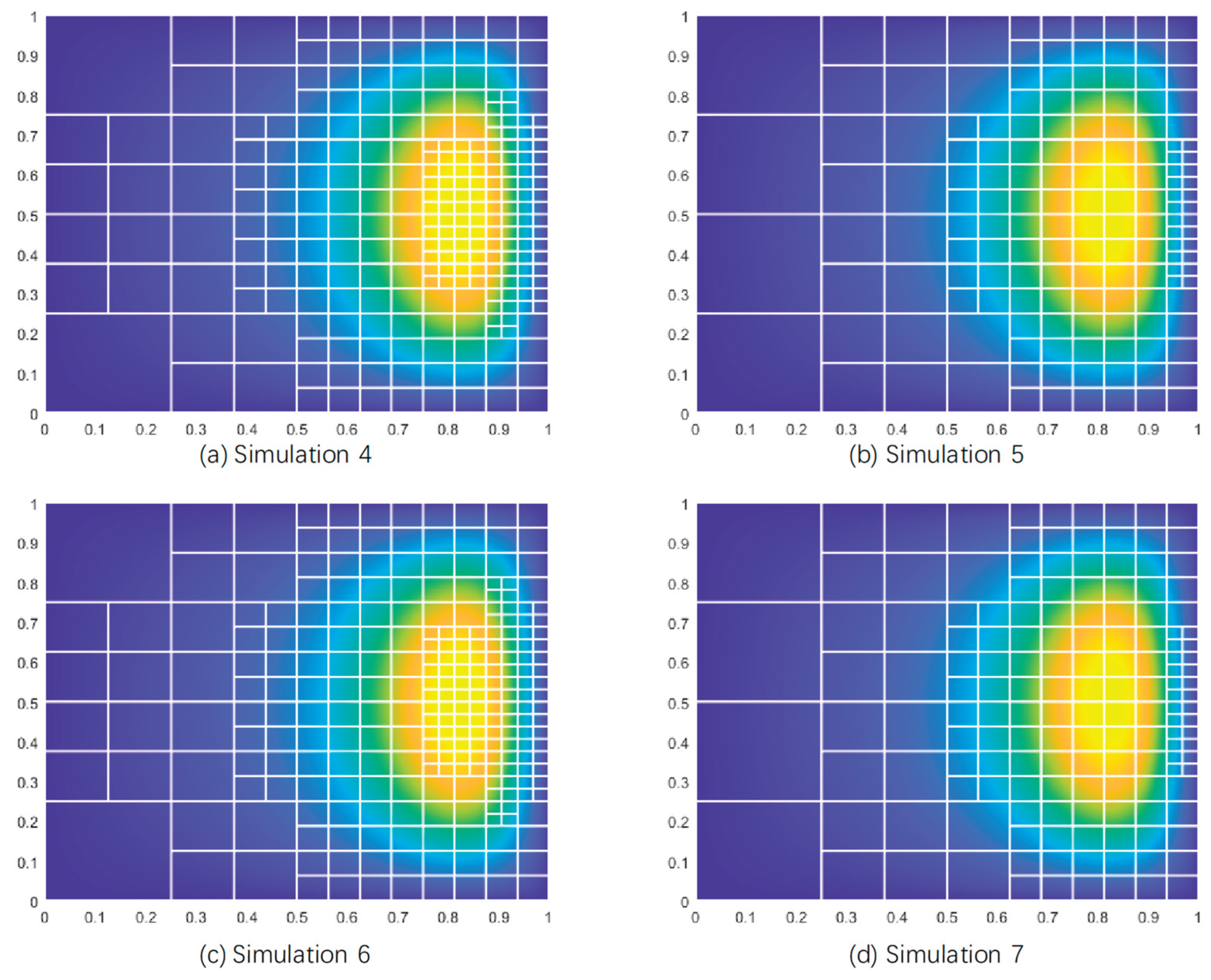
From the first two figures, it can be observed that the optimal pressure solutions achieved by different parameter combinations are approximately consistent, indicating that different parameter combinations have minimal impact on the optimal pressure solution but significantly affect the degrees of freedom. Comparison reveals that Simulation 7 requires the fewest degrees of freedom to approach the optimal pressure solution, closely followed by Simulation 5, with the hierarchical clustering method being the most influential parameter affecting the degrees of freedom. The third figure shows that all methods achieve prioritized refinement of critical elements, and the refinement results correspond to the DOFS values. Therefore, parameter settings with fewer degrees of freedom, such as those in Simulations 5 and 7, are preferred. This study selects the parameter settings of Simulation 7 as the optimal configuration.
Different clustering methods also directly impact classification results and refinement efficiency. K-means and hierarchical clustering are commonly used clustering methods. The advantages of K-means include fast computation speed, suitability for large-scale datasets, and ease of implementation, as it quickly converges by dividing data into a fixed number of clusters. Hierarchical clustering, on the other hand, does not require a predefined number of clusters and can reveal the hierarchical structure of data, making it suitable for complex datasets. Therefore, two groups of comparative simulations were conducted to evaluate the results, with hierarchical clustering parameters set according to Simulation 7, K-means using the squared Euclidean distance metric, and cluster settings kept consistent.
Table 5.
Comparison of Different Clustering Methods.
| Simulation Group | Clustering Methods |
| 8 | hierarchical clustering |
| 9 | K-means |
Figure 12.
The Effect of Different Clustering Methods on the S Value
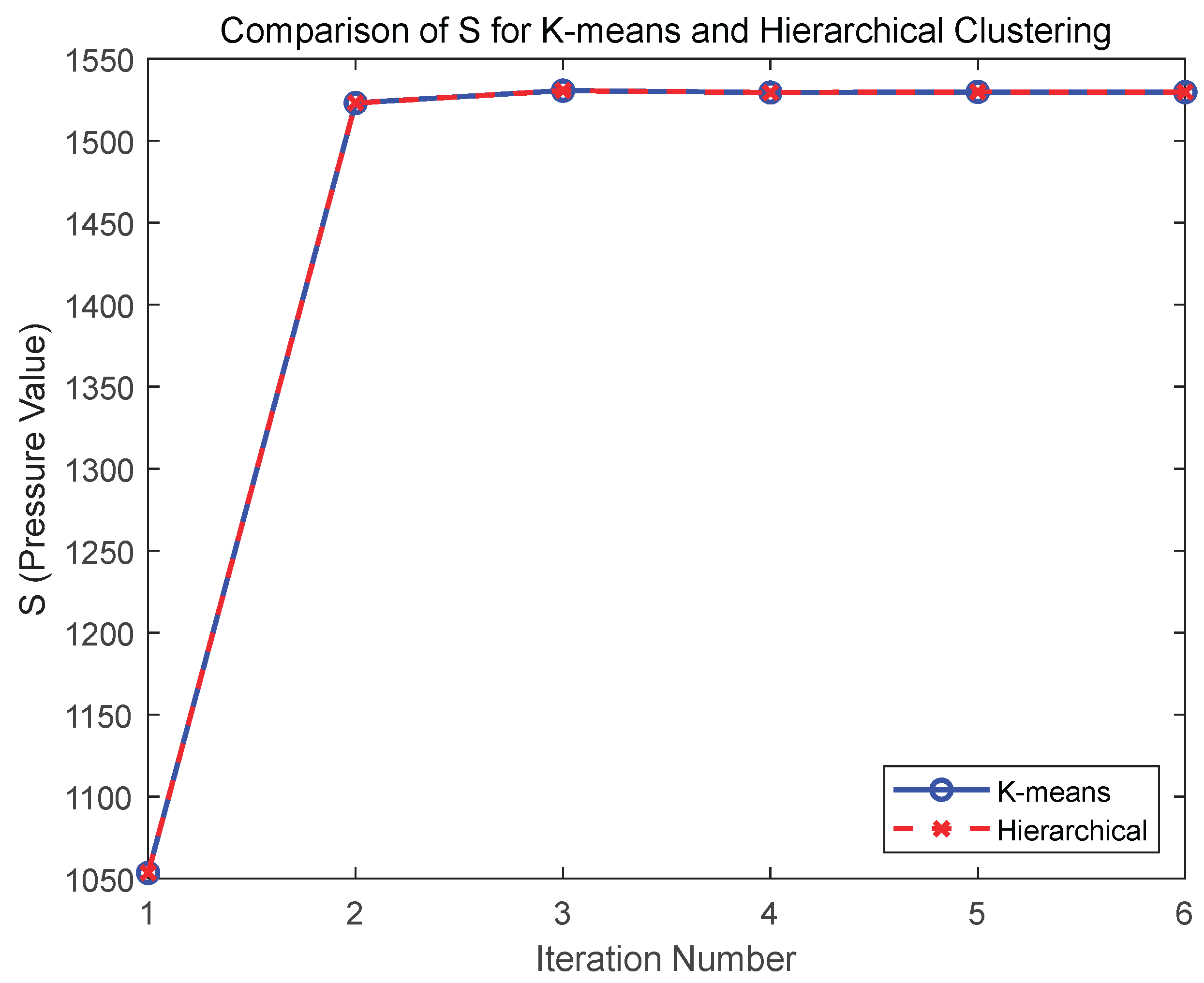
Figure 13.
The Effect of Different Clustering Methods on the DOFS Value
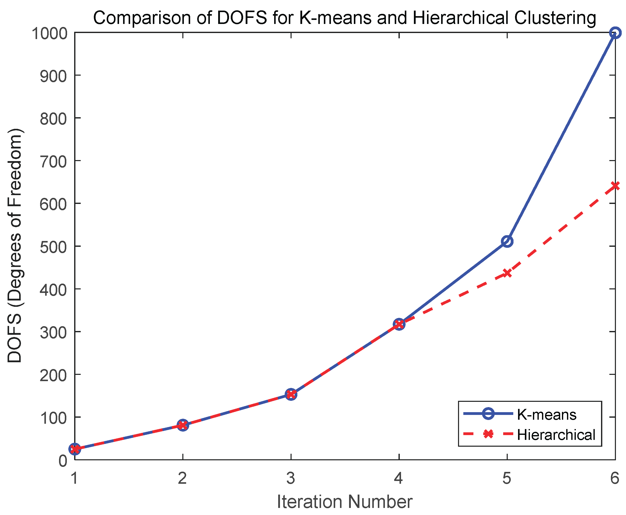
Figure 14.
Iterative Results of Mesh Refinement for Different Clustering Methods.
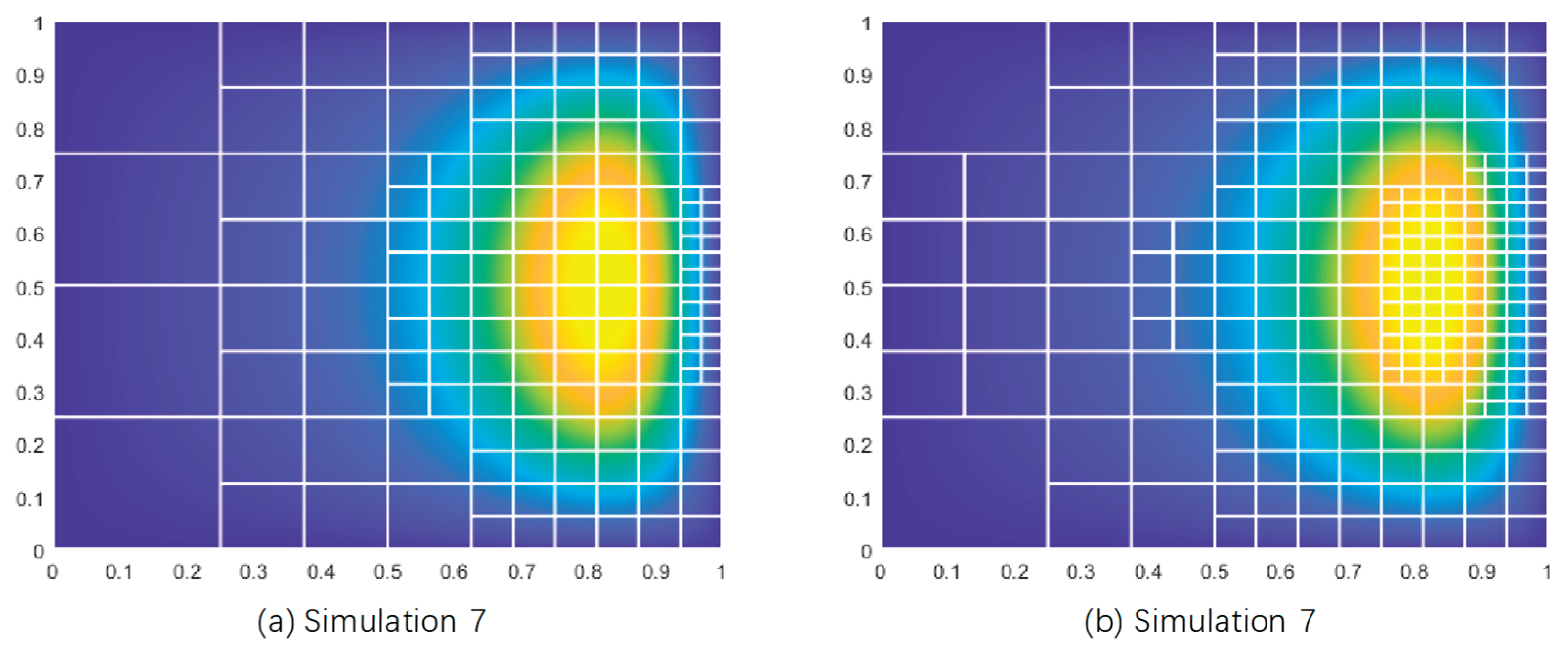
Analysis of the first two figures indicates that both K-means and hierarchical clustering methods converge toward a similar optimal pressure solution (S) over six iterations, with minimal deviation (e.g., the difference between the fifth and sixth iterations is less than 0.2%). Notably, hierarchical clustering requires significantly fewer degrees of freedom (DOFS) to achieve this solution—437 versus 511 in the fifth iteration and 641 versus 999 in the sixth iteration—demonstrating superior resource utilization efficiency. In the third figure, the iterative mesh refinement results for both methods show that they effectively target critical elements for refinement with negligible differences. Consequently, the hierarchical clustering method, which requires fewer degrees of freedom, is selected as the preferred approach.
Through systematic data analysis and validation, a processing scheme combining nonlinear piecewise transformation based on the median with hierarchical clustering (optimal parameter combination: Complete linkage criterion and Cityblock distance metric) has been established, achieving optimized element classification and significantly improved efficiency. However, it should be emphasized that this parameter combination is not universally applicable, as its effectiveness is closely tied to the distribution characteristics of the input data. In practical applications, it is recommended to repeat the above analysis and validation process based on the statistical properties of specific datasets to ensure the adaptability and robustness of the parameter selection.
For the training data of the neural network, standardization is theoretically required again to facilitate learning and training. However, the aforementioned process already incorporates standardization. An alternative approach could involve introducing two sets of physical field data, standardizing each set individually, and then combining and re-standardizing them before inputting into the neural network for training. Specifically, data from the piston-cylinder system model are used, with physical field data varied by adjusting model parameters (using pressure data). The two datasets (each containing 16 element data points) are presented in the following table:
Table 6.
Element Pressure Data.
| Group | Element Number | Element Pressure Data | Element Absolute Scale |
| Group 1 | 1 | 8345.58 | 0.0625 |
| 2 | 8006.12 | ||
| 3 | 28253.74 | ||
| 4 | 26791.08 | ||
| 5 | 6843.65 | ||
| 6 | 3360.44 | ||
| 7 | 22306.58 | ||
| 8 | 10443.86 | ||
| 9 | 50587.60 | ||
| 10 | 47296.49 | ||
| 11 | 44740.59 | ||
| 12 | 40974.75 | ||
| 13 | 38420.35 | ||
| 14 | 17523.46 | ||
| 15 | 32276.93 | ||
| 16 | 14657.69 | ||
| Group 2 | 17 | 8366.28 | 0.0625 |
| 18 | 8023.26 | 0.0625 | |
| 19 | 28342.90 | 0.0625 | |
| 20 | 26862.18 | 0.0625 | |
| 21 | 6854.91 | 0.0625 | |
| 22 | 3364.72 | 0.0625 | |
| 23 | 22348.69 | 0.0625 | |
| 24 | 10460.20 | 0.0625 | |
| 25 | 32396.93 | 0.0625 | |
| 26 | 11508.25 | 0.015625 | |
| 27 | 11355.72 | 0.015625 | |
| 28 | 14138.73 | 0.015625 | |
| 29 | 13917.93 | 0.015625 | |
| 30 | 11024.15 | 0.015625 | |
| 31 | 10441.03 | 0.015625 | |
| 32 | 13447.59 | 0.015625 |
Data from different physical fields are first standardized individually and then combined for hierarchical clustering analysis. The combined dataset is standardized again, followed by a second hierarchical clustering analysis. The results are shown in the figure below:
Figure 15.
Comparison of Classification Results between Single and Double Standardization.
The results indicate that the classification outcomes remain unchanged after a dataset undergoes both the first and second standardization processes. This suggests that the two standardization processes have no impact on the classification positions of the data, with highly consistent classification results. Therefore, in the context of this study, the first standardization is sufficient to meet the requirements for data consistency and classification, and the second standardization does not provide additional improvements in classification. Consequently, secondary standardization is unnecessary.
Through the above process, the optimal nonlinear transformation method and clustering method were ultimately determined, forming a complete feature-based refinement method. However, refinement based on labeled methods has the drawback of low efficiency, as it requires computing element data and defining and classifying labels for each element in every iteration. If raw natural features could be directly input for refinement decisions, the refinement efficiency could be significantly improved. Neural networks align with this approach and can serve as an efficient tool to accelerate the implementation of refinement decisions.
3.4. Neural Network-Based Feature Recognition Algorithm
The entire refinement process of IGA is executed sequentially, meaning that whenever the physical field or parameters change, a new algorithm must be redesigned for classification and refinement, resulting in low efficiency. While adopting parallel processing can improve computational efficiency, parallel methods have poor generalizability, and adjustments to the algorithm are still required whenever parameters or conditions change. To address this issue, machine learning methods can effectively replace traditional labeling and classification processes. Regardless of changes in the physical field or parameters, machine learning methods can automatically perform element refinement decisions by extracting standardized element feature data. This not only simplifies the entire process but also significantly enhances processing efficiency through CPU computation, resolving the flexibility and efficiency bottlenecks of traditional methods.
Among machine learning methods, neural networks are widely adopted due to their superior performance in classification and prediction tasks. In particular, neural networks introduce nonlinearity through activation functions such as Sigmoid[34], enabling effective fitting of complex nonlinear relationships and extraction of key features or patterns from high-dimensional data. Their multi-layer structure allows adaptive learning of complex patterns, capturing underlying regularities through nonlinear transformations without requiring manual feature engineering. The deep architecture excels at extracting hierarchical features, making it suitable for complex data such as images and text. Backpropagation and gradient descent algorithms enable efficient parameter tuning, adapting to diverse data distributions and achieving high prediction accuracy with sufficient data. This study selects neural networks as the primary model, though other machine learning methods are also applicable, and subsequent example validations will compare their performance.
During neural network training, the element information initially used consists of element information from the same physical field, with three key feature information of the element serving as the neural network input. To enhance algorithm efficiency, the input data is no longer the entire element data generated by interpolation but is instead composed of a column vector , formed by the pressure values at several Gauss quadrature points of a single element, the pressure gradient values in the x and y directions, and the absolute scale of the element. All elements are combined to form the dataset .
During neural network training, the element information used initially pertains to the same physical field, with three major element feature data as inputs to the neural network. To improve algorithmic efficiency, the input data are no longer the entire element data generated by interpolation but instead consist of column vectors formed by the pressure values at several Gaussian quadrature points of a single element, the pressure gradient values in the x and y directions, and the absolute scale of the element.
The neural network is trained using data generated by the method of element refinement based on feature labels. Additionally, to enhance the generalization of the neural network model, the model parameters are adjusted to incorporate element information from various physical fields for training.
Figure 16.
Neural Network Training Process.
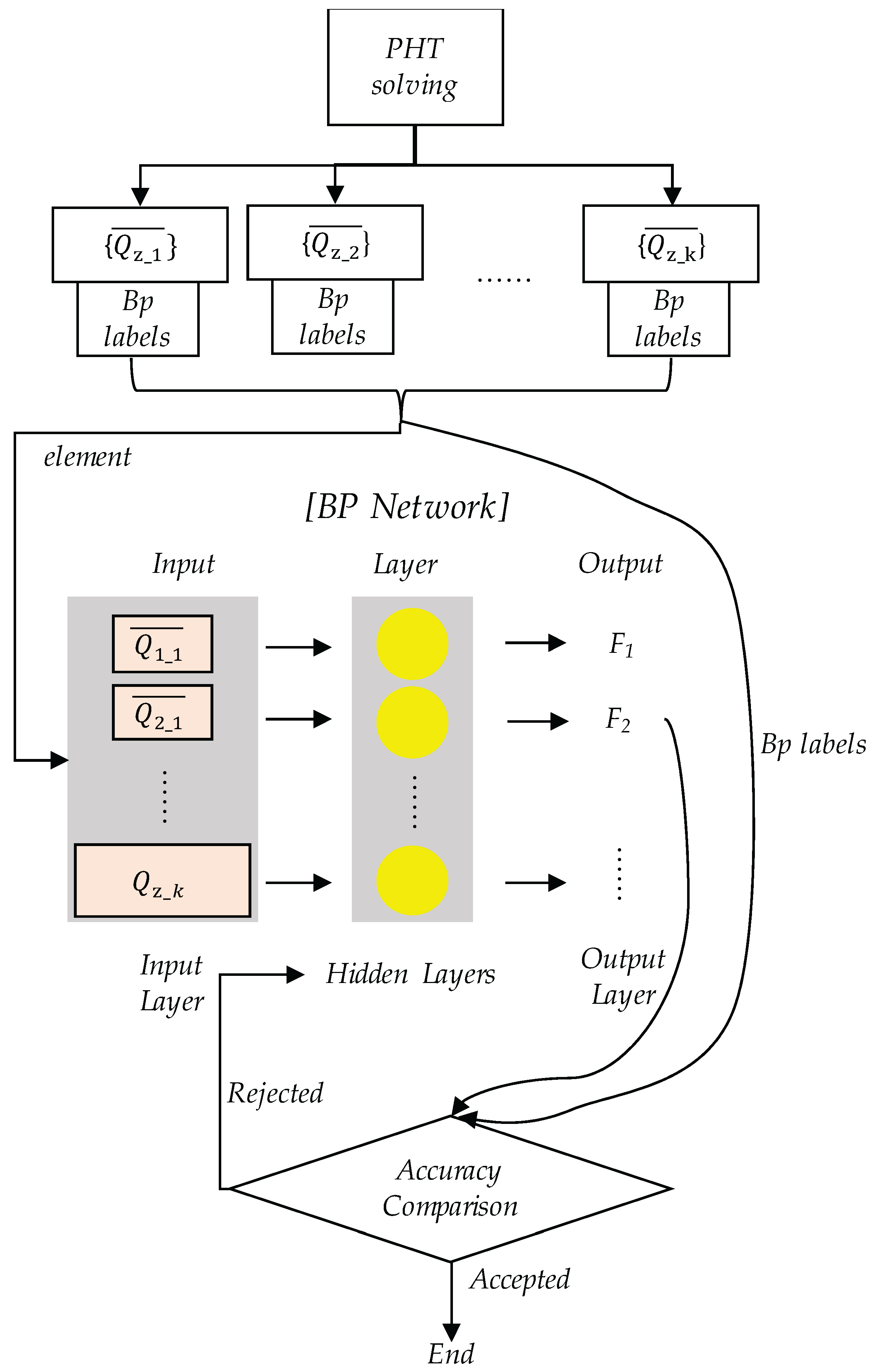
In the figure, F represents the element category, and k (k = 1, 2, 3, …) denotes different physical fields. By modifying model parameters to alter the physical field and following the process shown in Figure 5, element feature vectors under different conditions can be obtained. These vectors serve as inputs to train the neural network model, enhancing its applicability and accuracy.
Once the neural network achieves the desired training performance, it can be integrated into the algorithm as shown in the flowchart below.
In the figure, the refinement results for the physical domain and parameter domain are merely illustrative and do not represent actual results. The flowchart in Figure 17 outlines the overall process of feature recognition based on neural networks. After inputting feature data into the neural network, the BP (backpropagation) neural network can predict the categories of all elements, thereby determining the corresponding refinement decisions. Compared to Figure 5, the neural network effectively replaces the classification and labeling processes.
The results of element refinement are shown in Figure 18:
In Figure 18, (a) shows a two-dimensional refinement result of a physical field element, and (b) shows a three-dimensional result. The closer to the yellow region, the higher the element pressure value, indicating that the highest refinement level should be in the yellow region, while the lowest refinement level should be in the dark blue region on the left. In the refinement result shown in (a), this logic is satisfied, demonstrating the rationality of the refinement logic. Similarly, in areas with significant pressure changes, i.e., regions with large pressure gradients, refinement is also required. In the three-dimensional refinement result shown in (b), it is clear that elements with x-direction scales in the range [0.5, 0.8] exhibit significant pressure gradient changes in the x-direction, necessitating refinement. The result in (b) also aligns with this logic, further confirming the rationality of the refinement logic.
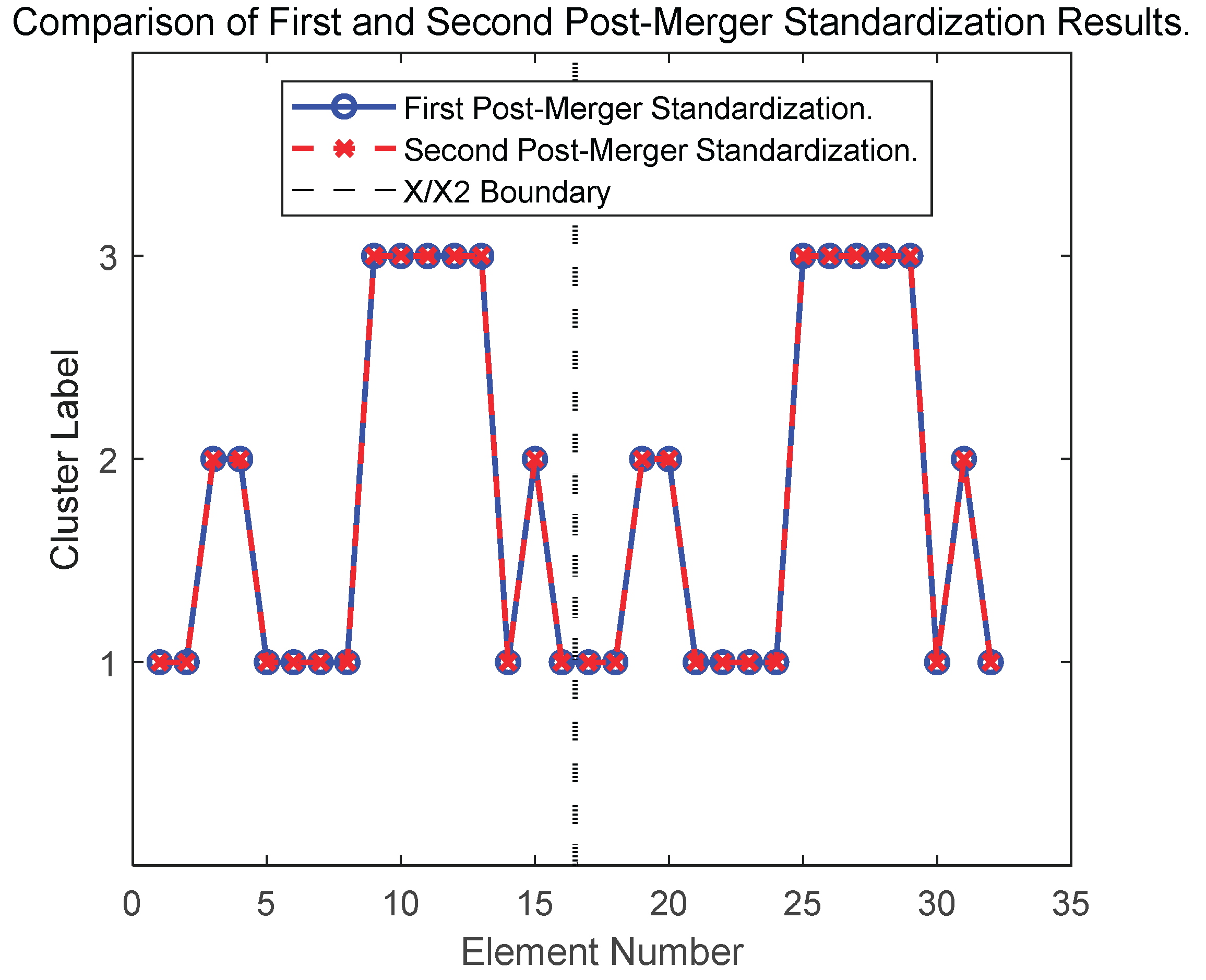
After verifying the rationality of the refinement logic of the feature recognition algorithm based on neural networks, the feature classification-based refinement method is applied to the same physical field element, and the refinement results of both methods are compared to validate the correctness of the algorithm. To ensure a fair comparison, both methods use the same number of refinements. The refinement results based on feature classification are shown in Figure 19. Comparing Figure 18 and Figure 19, it is evident that the refinement results of both methods are highly consistent, confirming the correctness of the neural network model.
Next, a complete refinement process is implemented using the feature recognition algorithm based on neural networks, with the results shown in the figure below:
The algorithm underwent nine iterations, clearly demonstrating that the neural network-based feature recognition algorithm can efficiently and accurately identify critical elements. The results show that the neural network model exhibits stable performance across multiple refinements, successfully identifying critical features in the target mesh elements, with the recognition results of each iteration highly consistent with expectations. This not only validates the correctness and reliability of the algorithm in the task of identifying critical elements but also lays a solid foundation for subsequent algorithm optimization and its application in similar scenarios.
3.4.1. Neural Network Model Parameter Selection and Adaptive Tuning
The performance of neural network models heavily depends on the selection of model parameters, including network architecture, optimizer, learning rate, regularization strategy, and batch size, among other key factors. The network architecture, typically determined by the number of hidden layers and their neuron counts, directly affects the model’s ability to capture data features. The optimizer (e.g., Adam, SGDM, or RMSProp) dictates the weight update strategy, influencing convergence speed and stability. The learning rate controls the step size of parameter updates, requiring a balance between convergence speed and training stability. Additionally, regularization methods (e.g., L2 regularization) and batch size play critical roles in the model’s generalization ability and training efficiency. Properly configuring these parameters is essential for enhancing the predictive accuracy and generalization capability of neural networks.
First, a baseline model (Model 1) is established with the following parameter configuration: 2 hidden layers with 16 and 8 neurons, respectively, a learning rate of 0.001, a batch size of 40, the Adam optimizer, an L2 regularization coefficient of 0, and a dataset split of 70%/10%/20%. The input data consists of 28-dimensional row vectors. The two-layer hidden structure, with 16 neurons in the first layer, effectively extracts key features from the 28-dimensional input, while the second layer with 8 neurons further compresses information, reducing the risk of overfitting while maintaining moderate model complexity. A learning rate of 0.001 is a commonly used initial value, and a batch size of 40 balances training efficiency and gradient stability. The Adam optimizer, leveraging the advantages of momentum and RMSProp, ensures fast and stable convergence. The dataset split of 70% for training, 10% for validation, and 20% for testing follows standard practice, with 70% ensuring sufficient training, 10% for parameter tuning, and 20% for evaluating generalization, providing a reliable baseline. Based on this, five groups of neural network models with different parameter configurations are compared to systematically evaluate the impact of each parameter on model performance, thereby selecting a more optimal parameter setting.
Table 7.
Settings of Neural Network Models with Different Parameter Configurations.
| Model | Number of Hidden Layers | Number of Neurons per Layer | Learning Rate | Batch Size | Optimizer | L2 Regularization Coefficient | Dataset Split |
| Model 1 | 2 | 16,8 | 0.001 | 40 | Adam | 0 | 70%/10%/20% |
| Model 2 | 3 | 32,24,16 | 0.01 | 80 | SGD with Momentum | 0.001 | 60%/20%/20% |
| Model 3 | 1 | 48 | 0.0001 | 20 | RMSProp | 0 | 80%/10%/10% |
| Model 4 | 4 | 64,32,16,8 | 0.001 | 160 | Adam | 0.01 | 70%/10%/20% |
| Model 5 | 2 | 24,12 | 0.1 | 40 | SGD with Momentum | 0 | 60%/20%/20% |
The models are comprehensively evaluated based on the root mean square error (RMSE) of the training and validation sets and the prediction accuracy of the test set output. The results are shown in the figure below:
Figure 21.
Root Mean Square Error of the Training Set
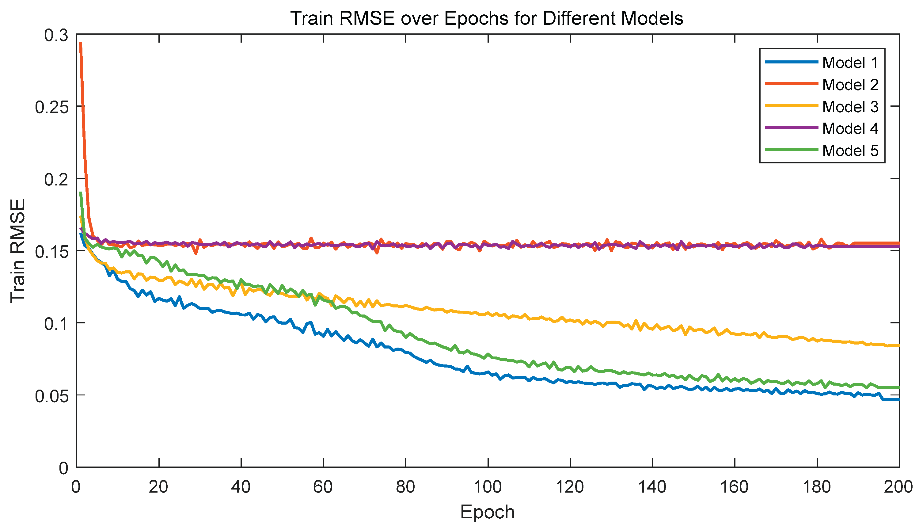
Figure 22.
Root Mean Square Error of the Validation Set.
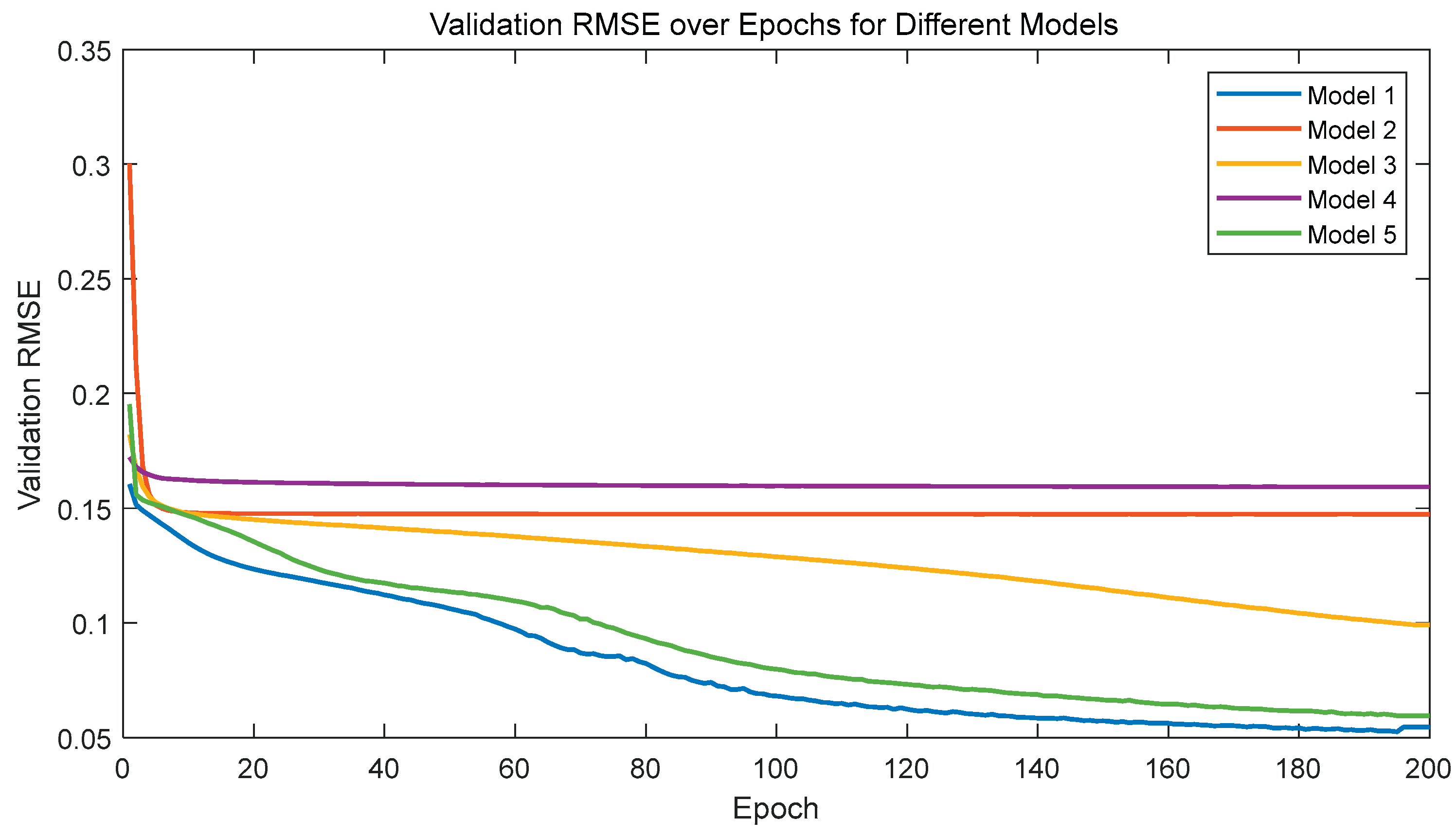
Figure 23.
Output Accuracy of Models with Different Parameter Configurations.
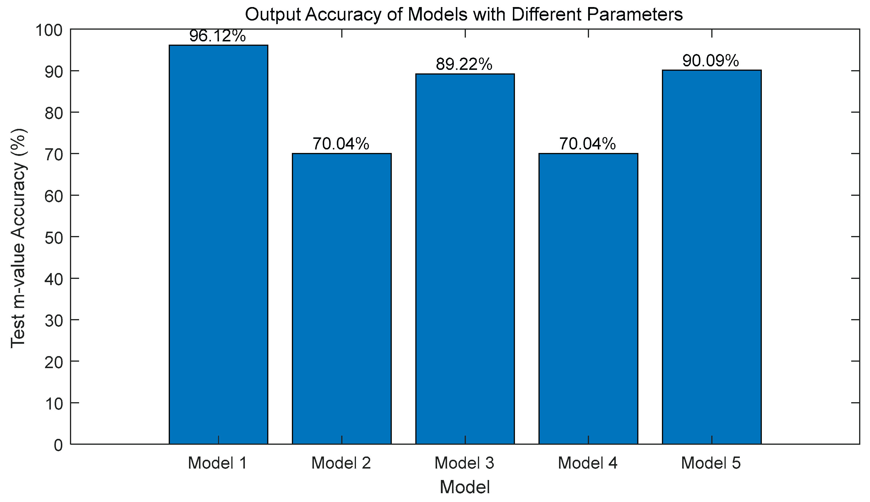
Analysis of the above figures reveals that Model 1 (2-layer network, Adam optimizer, learning rate of 0.001) performs exceptionally well across all metrics, with the lowest training RMSE, a validation RMSE of approximately 0.05, and a test set output accuracy of up to 96.12%, significantly outperforming other models.
In addition to the above parameters, batch normalization is a critical technique in neural network architecture design, effectively enhancing training stability and prediction accuracy. Therefore, a batch normalization layer is introduced during the neural network construction process to further optimize model performance. By comparing the differences in refinement results between models with and without batch normalization, the specific impact of batch normalization on model accuracy can be systematically evaluated.
Figure 24.
Comparison of the Impact of Batch Normalization on Element Refinement Results in Neural Networks.
Figure 24.
Comparison of the Impact of Batch Normalization on Element Refinement Results in Neural Networks.
In the figure, the left column displays the element refinement results predicted by the neural network model without batch normalization, while the right column shows the results predicted by the neural network model with batch normalization. A comparison of the refinement result figures indicates that the two are highly similar, suggesting that batch normalization has a limited impact on the predictive performance and element refinement results of the current neural network. However, the refinement results in the left column are structurally more standardized and rational. Therefore, based on the performance of the current model, batch normalization is not used.
Ultimately, the preliminary comparative analysis provides key references for subsequent parameter optimization. However, relying solely on the comparison of five model configurations may limit the results to locally optimal parameter combinations, making it difficult to further enhance model performance. Therefore, an adaptive approach is adopted to design a neural network algorithm capable of autonomously adjusting hyperparameters, as shown below, to explore a broader range of parameter combinations and gradually approach the globally optimal model.
Table 8.
Neural Network Refinement Algorithm for Autonomous Hyperparameter Adjustment.
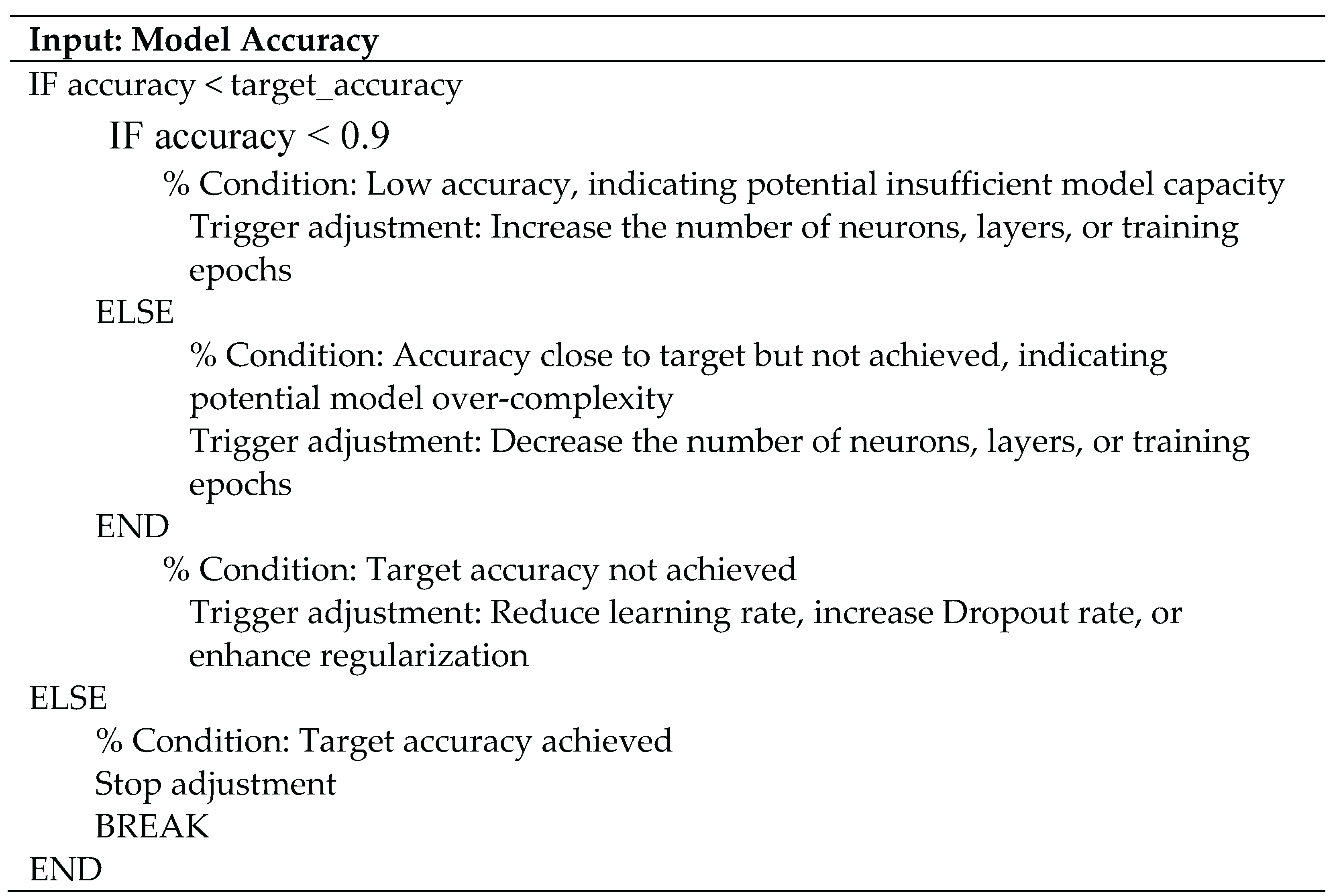
By evaluating model accuracy (whether the predicted element label values match the defined element label values), key neural network parameters are adaptively adjusted to obtain the optimal model. However, the process of tuning neural network parameters is complex and nearly infinite. Traversing all parameter combinations to find the globally optimal model requires extensive iterative computations, resulting in a substantial workload. Given that the preliminary design of this study has achieved a high model accuracy (96.12%), Model 1 already meets practical requirements. If a more optimal model is needed, further improvements can be made following the aforementioned algorithm.
Therefore, certain parameters of the neural network model in this study are set according to Model 1, followed by additional generalization training in accordance with the neural network training process. Subsequently, appropriate parameter tuning is conducted to obtain a neural network model with higher accuracy.
4. Algorithm Application
Through the aforementioned steps, a neural network model can be successfully constructed and trained to accurately perform feature recognition of element information and predict element categories. To validate the accuracy and robustness of the proposed algorithm, two independent neural network models (BP-1 and BP-2) were trained using the lubrication model of the piston-cylinder system and the hydrostatic sliding bearing model, respectively, for performance evaluation. To further investigate the generalization ability and cross-scenario adaptability of neural networks in refinement tasks for different lubrication problems, BP-1 was used to predict element categories for the hydrostatic sliding bearing model, and BP-2 was similarly used to predict element categories for the piston-cylinder system lubrication model, with model prediction accuracy and refinement results compared. Additionally, the data from both lubrication models were combined into a single dataset to train a new neural network model (BP-3). Generalization validation results demonstrate that BP-3, as a single model, can directly adapt to refinement tasks for various lubrication problems without requiring scenario-specific data preparation or dedicated model training, thereby significantly enhancing the model's versatility and application efficiency.
4.1. Lubrication Model of Piston-Cylinder System
Figure (a) shows the piston-cylinder liner configuration, and Figure (b) illustrates the oil film lubrication. denotes the crank radius; and denote the distances between the center of the piston skirt and the cylinder liner axis at the top and bottom of the skirt, respectively. denotes the piston skirt length.
Figure 25.
Schematic of Piston-Cylinder System and Lubrication Regions.
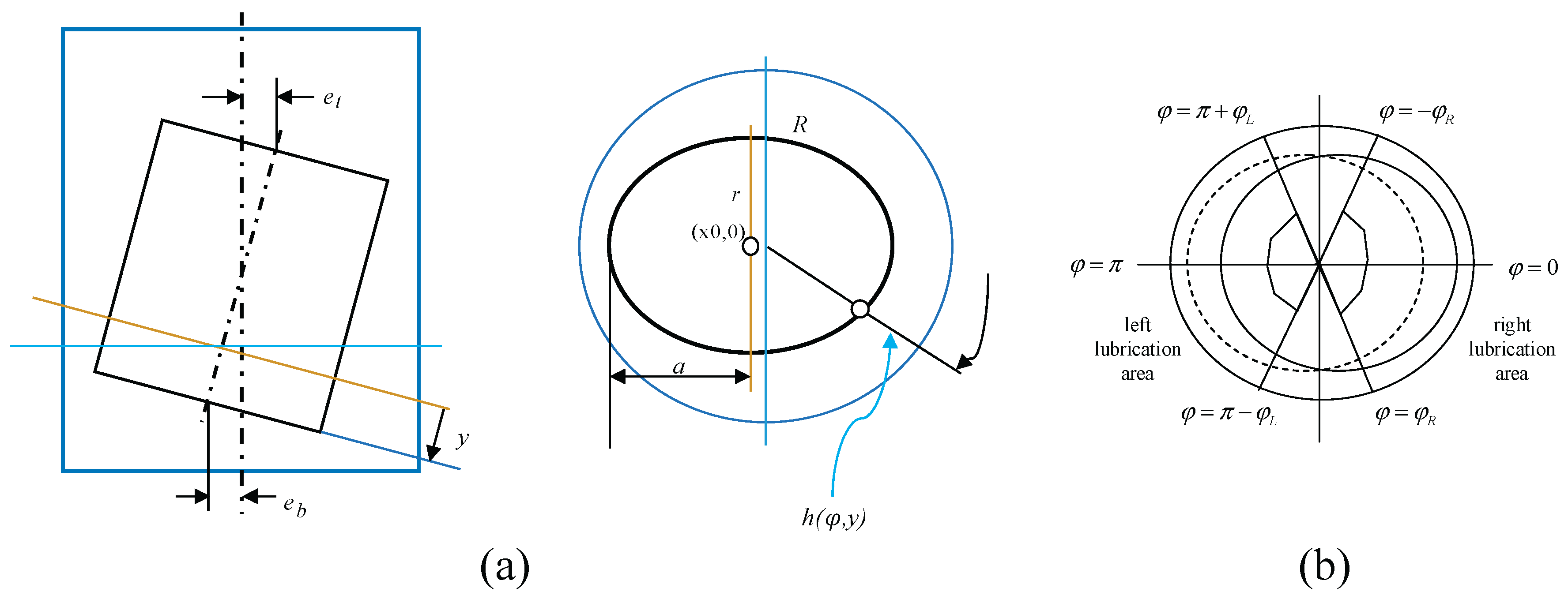
The morphology diagram in Figure 25a is obtained by solving a specific simplified Reynolds equation[35] based on the Navier-Stokes equations and the continuity equation.
In Equation (9), denotes time, denotes oil film pressure, denotes dynamic viscosity, and denote the circumferential velocities of the oil film on the piston and cylinder liner, respectively, and denote the axial velocities of the oil film on the piston and cylinder liner, respectively, denotes oil film thickness, and denotes lubricant density.
Figure 25b presents a simplified representation of the oil film lubrication region, divided into left and right lubrication zones, symmetric about the plane . Equation (9) is further simplified by assuming constant and , and neglecting leakage[36].
Take,,=,
The domain is mapped to the unit square using the following transformations (example shown for the right side):
The oil film thickness in Equation (11) can be calculated using an elliptical equation, such as Equation (12).
However, the IGA solution process requires a regular geometric domain, necessitating a transformation of the oil film lubrication region into a rectangular domain.
First, the piston-cylinder system with secondary piston motion is taken as an example, using the Reynolds boundary conditions[37]. Other boundary conditions are treated similarly, and the dynamic calculations are omitted for brevity. The input parameters, based on a specific single-cylinder gasoline engine, are listed in Table 9[38].
Figure 26.
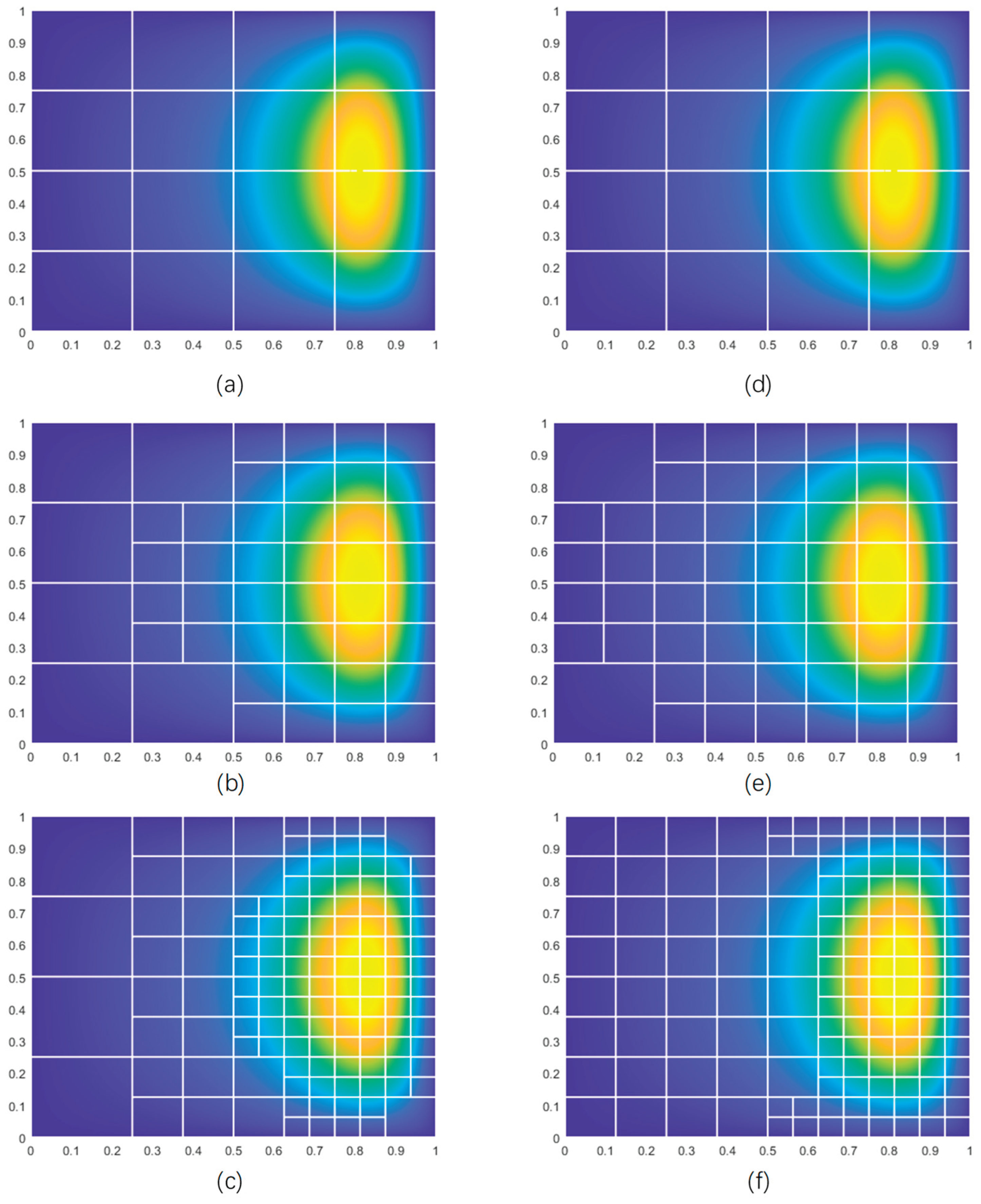
Comparison of feature classification before and after data processing.
The left column of the figure shows the feature classification results before data processing, and the right column shows the results after processing. (a) to (c) represent successive refinement steps, similarly for the right column.
From the figures, it can be observed that the method without data processing, from (a) to (c), performs large-scale refinement based on the previous level, failing to effectively identify critical elements. However, the method with data processing prioritizes the recognition and refinement of critical elements in each iteration, gradually expanding outward. This validates the necessity of data processing (here referring to standardization and differential amplification processing) as described in Section 3.2.
Table 10.
Comparison of Degrees of Freedom, Pressure Values, and Refinement Time for the Two Cases.
| Number of Refinements | Without Data Processing | With Data Processing | ||||||
| DOFs | Pressure(N) | Time(s) | DOFs | Pressure(N) | Time(s) | |||
| 3 | 217 | 183.3025 | 3.1273 | 217 | 183.3025 | 2.3790 | ||
| 4 | 769 | 183.5318 | 4.3321 | 727 | 183.5213 | 3.4891 | ||
| 5 | 2825 | 183.5509 | 6.1079 | 919 | 183.5328 | 4.7209 | ||
| 6 | 3829 | 183.5515 | 24.7455 | 1281 | 183.5443 | 6.1425 | ||
| 7 | 11703 | 183.5529 | 31.1459 | 1841 | 183.5499 | 7.8066 | ||
| 8 | 12869 | 183.5532 | 40.8508 | 2181 | 183.5510 | 9.5794 | ||
As shown in Table 6, the pressure value solutions obtained by the two refinement methods are similar. However, the method with data processing achieves comparable pressure value solutions with fewer degrees of freedom, indicating higher efficiency. Moreover, as the number of refinements increases, the time consumed by the method without data processing grows significantly, reaching approximately four times that of the method with data processing by the eighth refinement, which substantially reduces refinement efficiency.
In comparing these two methods, the input parameter , while other parameters remained consistent with Table 9. In Figure 27, the left column shows the 2D refinement results, and the right column shows the corresponding 3D results. (a) and (b) are the results using the PHT-IGA method; (c) and (d) are the results using the feature classification-based method. Figure (a) and (c) show that in areas with a large pressure gradient, the local method does not refine the region sufficiently, and for areas with high pressure, the local method's refinement is insufficient.
Table 11.
Comparison of Data Results.
| Number of Refinements | Without Data Processing | With Data Processing | ||||||
| DOFs | Pressure(N) | Time(s) | DOFs | Pressure(N) | Time(s) | |||
| 1 | 25 | 178.5365 | 0.0414 | 25 | 162.5501 | 0.0394 | ||
| 2 | 81 | 181.1382 | 1.9617 | 81 | 180.7430 | 1.6458 | ||
| 3 | 189 | 181.2513 | 3.2149 | 217 | 183.3025 | 2.3790 | ||
| 4 | 287 | 181.2525 | 4.3925 | 727 | 183.5213 | 3.4891 | ||
From the table, it can be observed that, under the same number of refinements, the feature classification-based method achieves a solution closer to the optimal pressure value and requires relatively less time per refinement. In comparison, the neural network-based feature recognition method demonstrates superior refinement performance.
Next, when comparing the feature classification method and the neural network-based feature recognition method, new feature data are directly used as input to the neural network to predict refinement results and conduct a comparison.
Figure 28.
Results of the Sixth Refinement for the Feature classification-Based Method and the Neural Network-Based Feature Recognition Method.
Figure 28.
Results of the Sixth Refinement for the Feature classification-Based Method and the Neural Network-Based Feature Recognition Method.
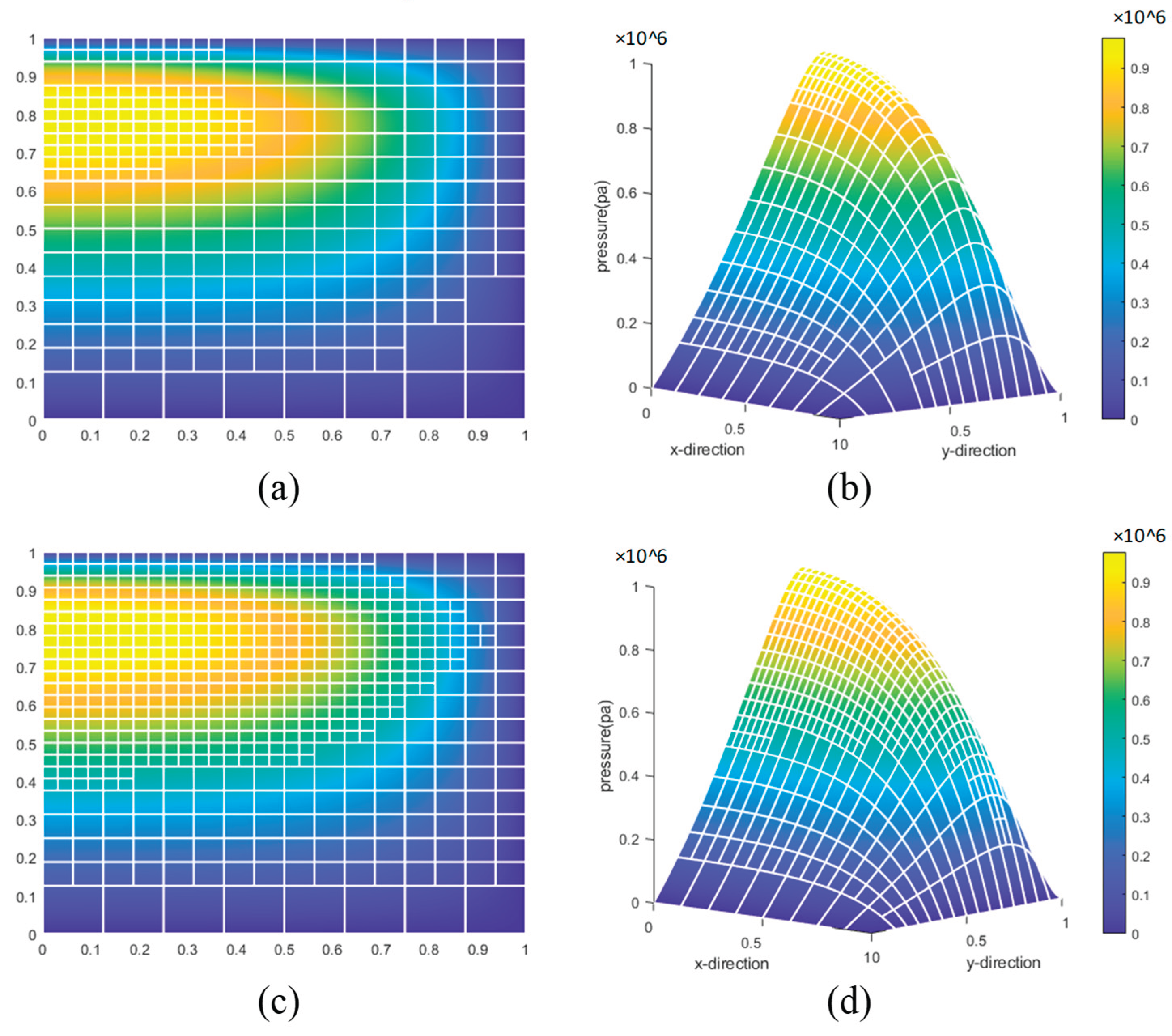
In the figure, (a) and (b) represent the results of the feature classification-based method, while (c) and (d) represent the results of the neural network-based feature recognition method, all obtained after six refinements. From the figure, it can be observed that the stable element pressure values obtained by both methods are very close, indicating that the neural network model can accurately predict the refinement of unknown elements.
Once the neural network model is completed, it can also be applied to mesh refinement in other physical fields. The parameter values are modified as shown in Table 12.
Figure 29.
Comparison of results from the neural network-based feature recognition method in different physical fields.
Figure 29.
Comparison of results from the neural network-based feature recognition method in different physical fields.
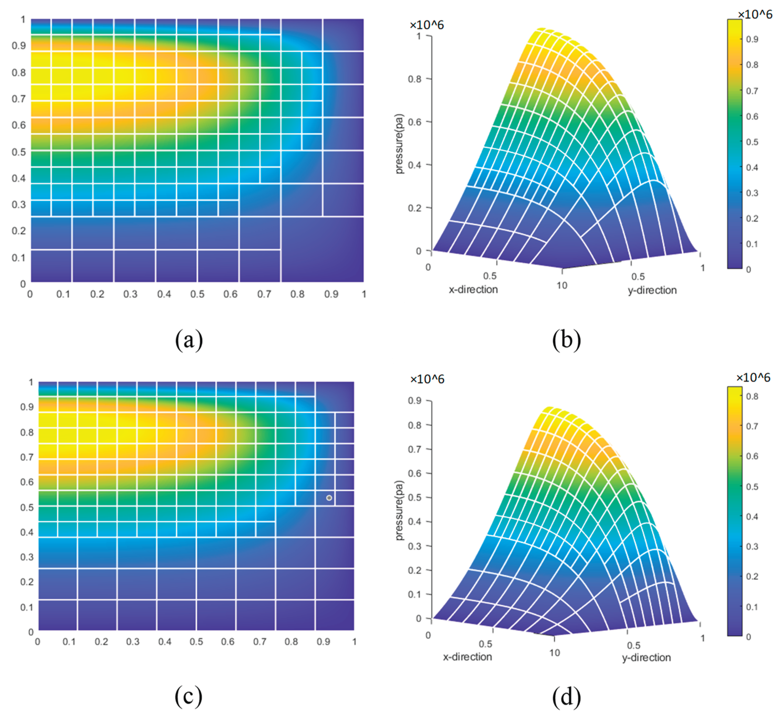
In the figure, (c) represents the two-dimensional refinement result of another physical field, and (d) illustrates the three-dimensional refinement result. From this, it can be inferred that the element pressure and pressure gradient across the entire new physical field have undergone changes. However, the neural network-based feature recognition method effectively identifies and refines regions in the new physical field with high absolute pressure values and significant pressure gradients. This indicates that the neural network model exhibits strong generalization capability.
The previous section mentioned that this example represents an initial attempt to apply a neural network method, but other machine learning methods are also applicable. In this example, Support Vector Machine (SVM)[39] is introduced as a new machine learning approach. SVM is a machine learning method based on margin maximization, which maps data to a high-dimensional space through the selection of appropriate kernel functions (e.g., linear kernel, Gaussian kernel, or polynomial kernel), making it suitable for both regression and classification tasks. Its key parameters include the kernel function type, kernel scale, regularization parameter, ε-insensitive loss parameter (Epsilon), and whether to standardize data (Standardize), among others. The choice of these parameters directly determines the model’s fitting capability and generalization performance. Similar to the parameter tuning of neural networks, we designed five sets of controlled simulation experiments to systematically compare the impact of different parameter combinations on SVM model performance, thereby determining the optimal parameter settings. The specific parameter configurations are shown in the table below:
Table 13.
SVM Settings for Different Parameter Models.
| Model | Kernel Function | Kernel Scale | Standardization | BoxConstraint (C) | Epsilon | Dataset Partition |
| Model 1 | Rbf | Auto | True | 1 | 0.037 | 70%/10%/20% |
| Model 2 | Linear | - | True | 0.1 | 0.05 | 60%/20%/20% |
| Model 3 | Polynomial | 3 | False | 10 | 0.2 | 80%/10%/10% |
| Model 4 | Rbf | 1 | True | 5 | 0.01 | 70%/10%/20% |
| Model 5 | Polynomial | 2 | True | 0.5 | 0.5 | 60%/20%/20% |
The SVM model is evaluated based on two metrics: predicted residual distribution and test set output accuracy. The results are shown in the figure below:
Figure 30 and Figure 31 illustrate the performance evaluation of five SVM models. Figure 30, depicting the residual distribution, shows that Model 1 and Model 4 exhibit the smallest prediction biases (with residuals concentrated between -0.1 and 0.1, peaking at a frequency close to 100), while Model 5 has the largest bias (with the widest residual distribution, ranging from -0.4 to 0.4). Figure 31, a bar chart of accuracy (m-value), indicates that Model 1 achieves the highest accuracy (97.47%), followed by Model 4 (94.94%), Model 2 (94.30%), and Model 3 (93.75%), with Model 5 having the lowest accuracy (72.78%), consistent with the residual distribution trend. This suggests that Model 1’s parameter settings are optimal, and thus, the SVM model parameters in this study are set according to Model 1.
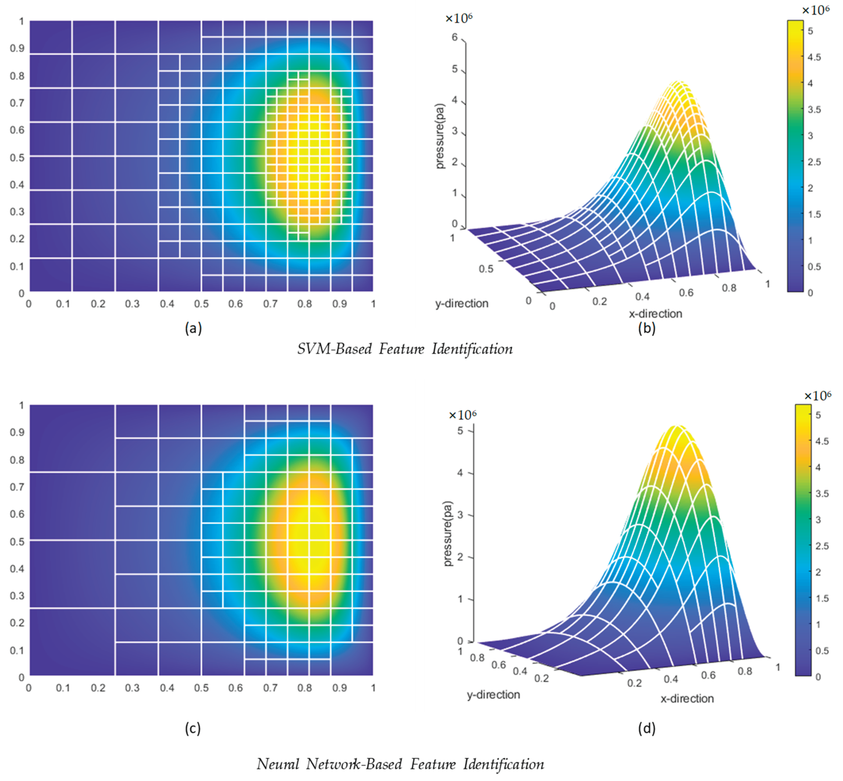
Under the same input conditions, the final cell refinement performance of the neural network and SVM methods is compared, with results shown in Figure 32:
In the figure, (a) and (b) represent the neural network method, while (c) and (d) represent the SVM method. It can be observed from the figure that the grid sparsity differs between the two methods. The SVM method fails to identify the lower-left region during refinement, but the overall cell refinement trend is similar to that of the neural network method, indicating that both methods can effectively capture data features. Based on the current simulation results, the neural network method demonstrates superior performance.
4.2. Hydrostatic Sliding Bearing Model
Here, denotes the external applied load; represents the angular velocity of the shaft; indicates the attitude angle; signifies the geometric center of the bearing center; and denotes the geometric center of the shaft center. Figure 33(a) depicts the bearing in a non-operating state, 33(b) illustrates the bearing in an operating state, and 33(c) shows a schematic diagram of the oil film pressure distribution.
Taking this model as an example, the two-dimensional steady-state incompressible flow pressure lubrication Reynolds equation under laminar flow conditions is formulated as follows:
In the equation, represents the oil film thickness; denotes the oil film pressure; and indicates the dynamic viscosity of the lubricating oil.
Let and in the equation, where and . Performing variable substitution yields:
Further let , where and . After simplification, it yields:
The parameters of the radial sliding bearing model for this example are shown in the table below:
Table 14.
Parameters of the Hydrostatic Sliding Bearing Model.
| Parameter | Description | Worth | Element |
| Radial clearance | |||
| Rotational speed | |||
| Bearing inner diameter | |||
| Bearing width | |||
| Viscosity | |||
| Eccentricity | |||
| Angular velocity | |||
| Angle |
Table 15.
Comparison of Degrees of Freedom and Pressure for Unprocessed and Processed Data Methods.
| Number of Refinements | Without Data Processing | With Data Processing | ||||||
| DOFs | Pressure(N) | Time(s) | DOFs | Pressure(N) | Time(s) | |||
| 1 | 25 | 1053.4 | 0.0414 | 25 | 1053.4 | 0.0519 | ||
| 2 | 81 | 1523 | 1.4326 | 81 | 1523 | 1.3354 | ||
| 3 | 203 | 1529.1 | 3.8336 | 153 | 1530.5 | 3.0211 | ||
| 4 | 557 | 1529.6 | 4.4012 | 487 | 1529.9 | 4.2153 | ||
| 5 | 1967 | 1529.4 | 6.3218 | 881 | 1529.6 | 5.1384 | ||
| 6 | 7205 | 1529.4 | 28.2372 | 1161 | 1529.6 | 6.3547 | ||
Table 16.
Modified Parameters.
| Parameter | Description | Worth | Element |
| Radial clearance | |||
| Rotational speed | |||
| Eccentricity |
Figure 34.
Refinement result comparison without and with data processing.
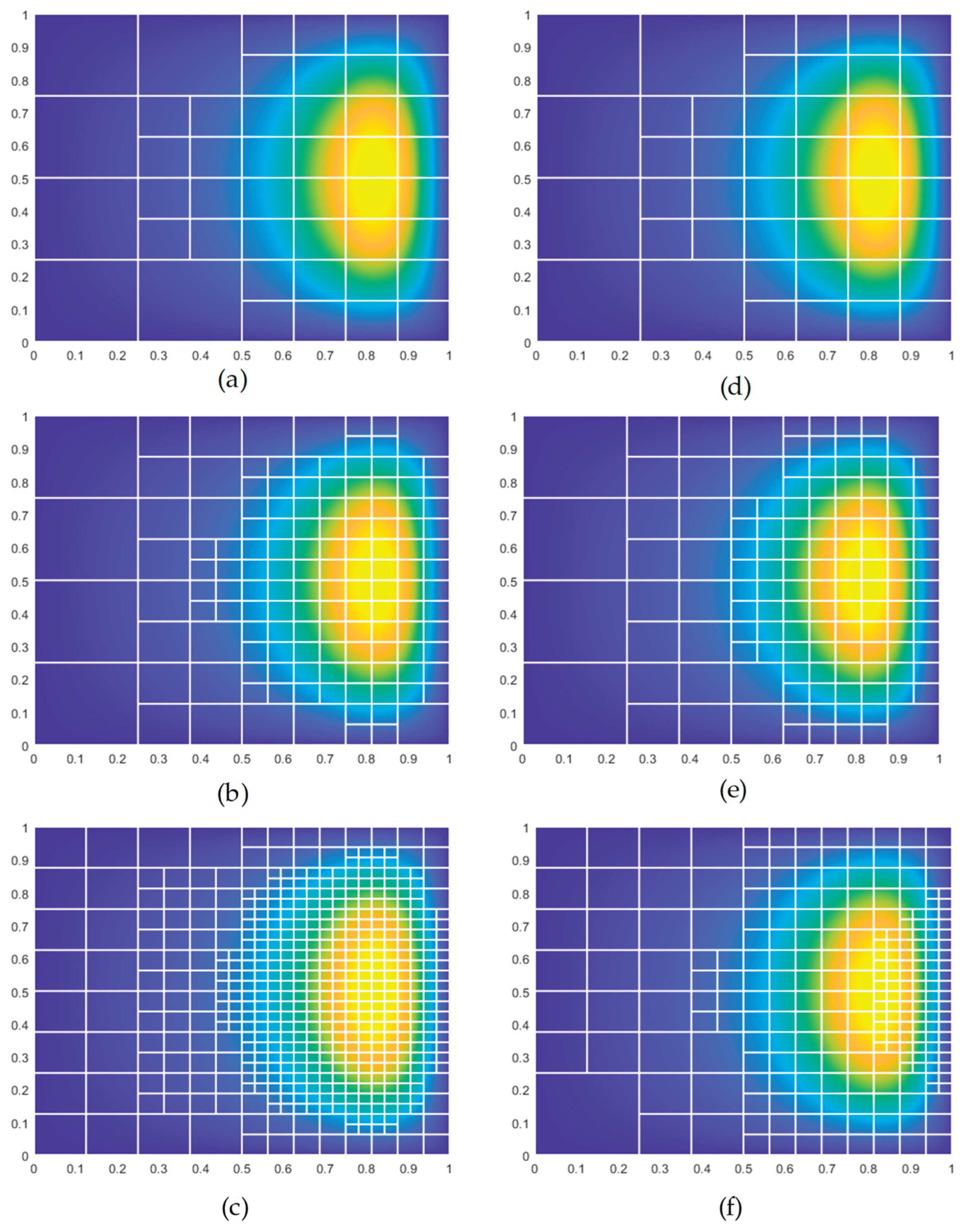
Figure 35.
Results Comparison of Feature classification Method and Neural Network Method.
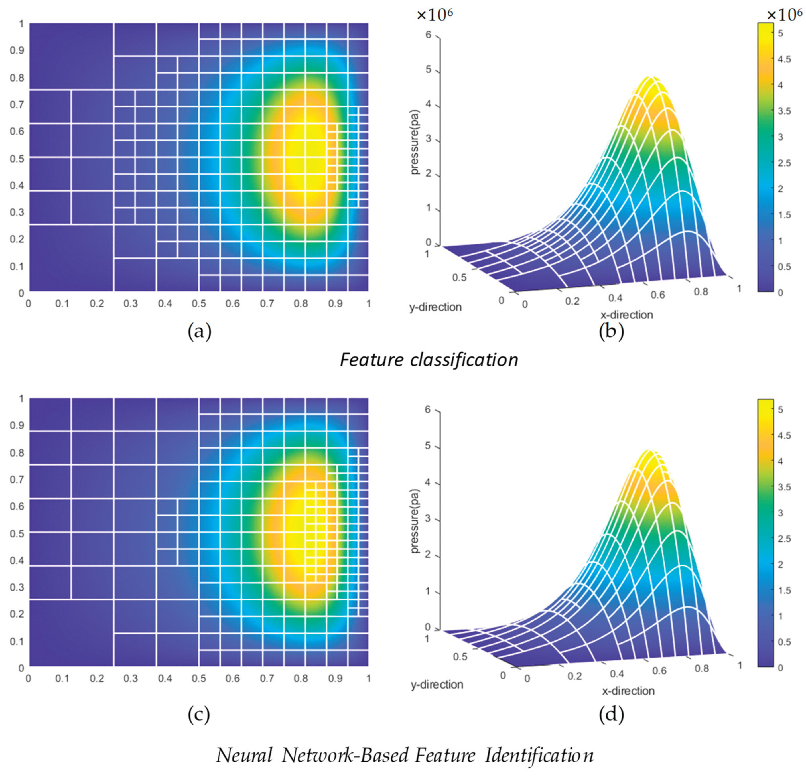
Figure 36.
Comparison of refinement results for the new and original physical fields.
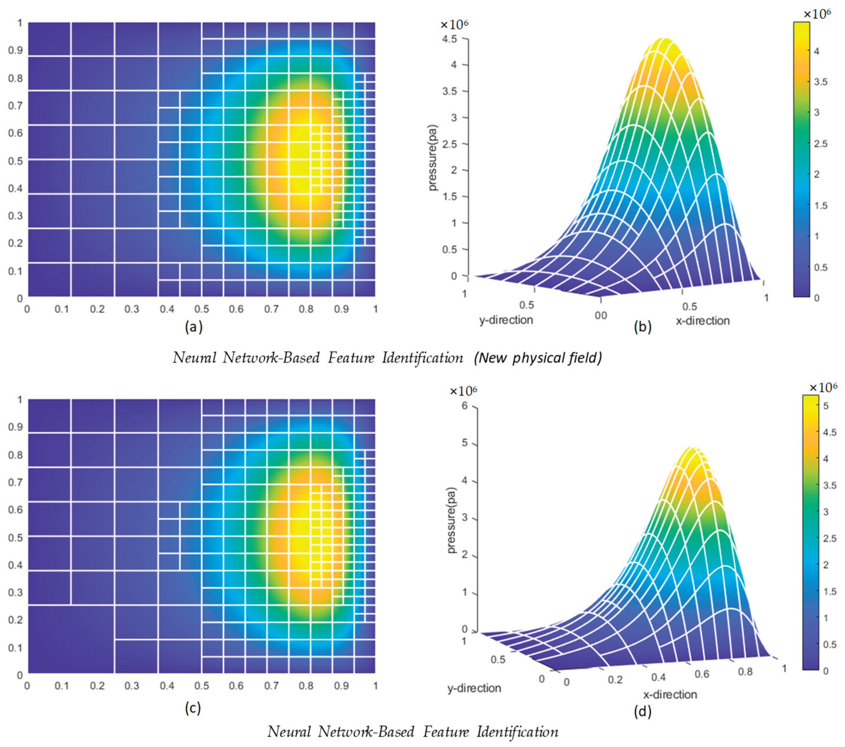
Figure 37.
Comparison of the neural network-based feature recognition method and the Support Vector Machine (SVM)-based feature recognition method.
Figure 37.
Comparison of the neural network-based feature recognition method and the Support Vector Machine (SVM)-based feature recognition method.
The model parameters were adjusted as shown in the table below, and the modified model was used to generate a new physical field for comparison.
The figures and tables presented above illustrate comparative refinement results under various scenarios. These results demonstrate that the neural network-based feature recognition method exhibits superior adaptability and generalization capability across diverse model configurations. It is noteworthy that, although the SVM and neural network methods exhibit significant differences in the degrees of freedom of the solved elements after the same number of refinement iterations, the computed pressure values are remarkably similar.
4.3. Generalization Validation
This section aims to validate the generalization ability and cross-scenario adaptability of neural networks in refinement tasks for different lubrication problems. Element feature data from two lubrication models (approximately 800 samples each) were collected, denoted as Dataset 1 and Dataset 2, respectively. First, Dataset 1 was used as input to invoke BP-2 for predicting element categories; similarly, Dataset 2 was used as input to invoke BP-1 for predicting element categories. The prediction accuracy was compared with that of the neural network model trained on the corresponding lubrication model. The results are shown in the table below:
Table 17.
Comparison of Prediction Accuracy for BP Models Across Different Lubrication Models.
| Neural network model | Lubrication model | Prediction accuracy |
| BP-1 | Piston-cylinder system | 94.55% |
| BP-2 | Hydrostatic sliding bearing | 70.85% |
| BP-1 | Piston-cylinder system | 75.25% |
| BP-2 | Hydrostatic sliding bearing | 96.95% |
Based on the table results, the current BP models demonstrate a certain degree of cross-scenario adaptability. BP-1 achieves an accuracy of 94.55% on the piston-cylinder system (Dataset 1) but drops to 70.85% when predicting the hydrostatic sliding bearing (Dataset 2). Similarly, BP-2 achieves an accuracy of 96.95% on the hydrostatic sliding bearing (Dataset 2) but only 75.25% when predicting the piston-cylinder system (Dataset 1). The decline in prediction accuracy in new scenarios indicates that the generalization ability of the BP models is still limited. By optimizing the model structure or training with a mixed dataset, the adaptability and prediction accuracy of neural networks across different lubrication problems can be further enhanced.
Following this approach, a neural network can be trained using mixed data. Datasets 1 and 2 were combined as training data, ensuring consistent proportions of data from both lubrication models across training, testing, and validation sets, to train BP-3. Subsequently, parameters of the two lubrication models were adjusted to generate Datasets 4 and 5 (approximately 750 samples each). BP-3 was applied to predict element categories in these datasets, and the model’s accuracy was evaluated. The results are shown in the table below:
Table 18.
Comparison of Prediction Accuracy for BP-3 Across Different Lubrication Models.
| Neural network model | Lubrication model | Prediction accuracy |
| BP-3 | Piston-cylinder system | 95.72% |
| BP-3 | Hydrostatic sliding bearing | 96.69% |
According to the table results, BP-3, after training on a mixed dataset, demonstrates strong generalization ability. It achieves an accuracy of 95.72% for the piston-cylinder system (Dataset 4) and 96.69% for the hydrostatic sliding bearing (Dataset 5), indicating that the single model BP-3 can effectively adapt to different lubrication scenarios with high prediction accuracy.
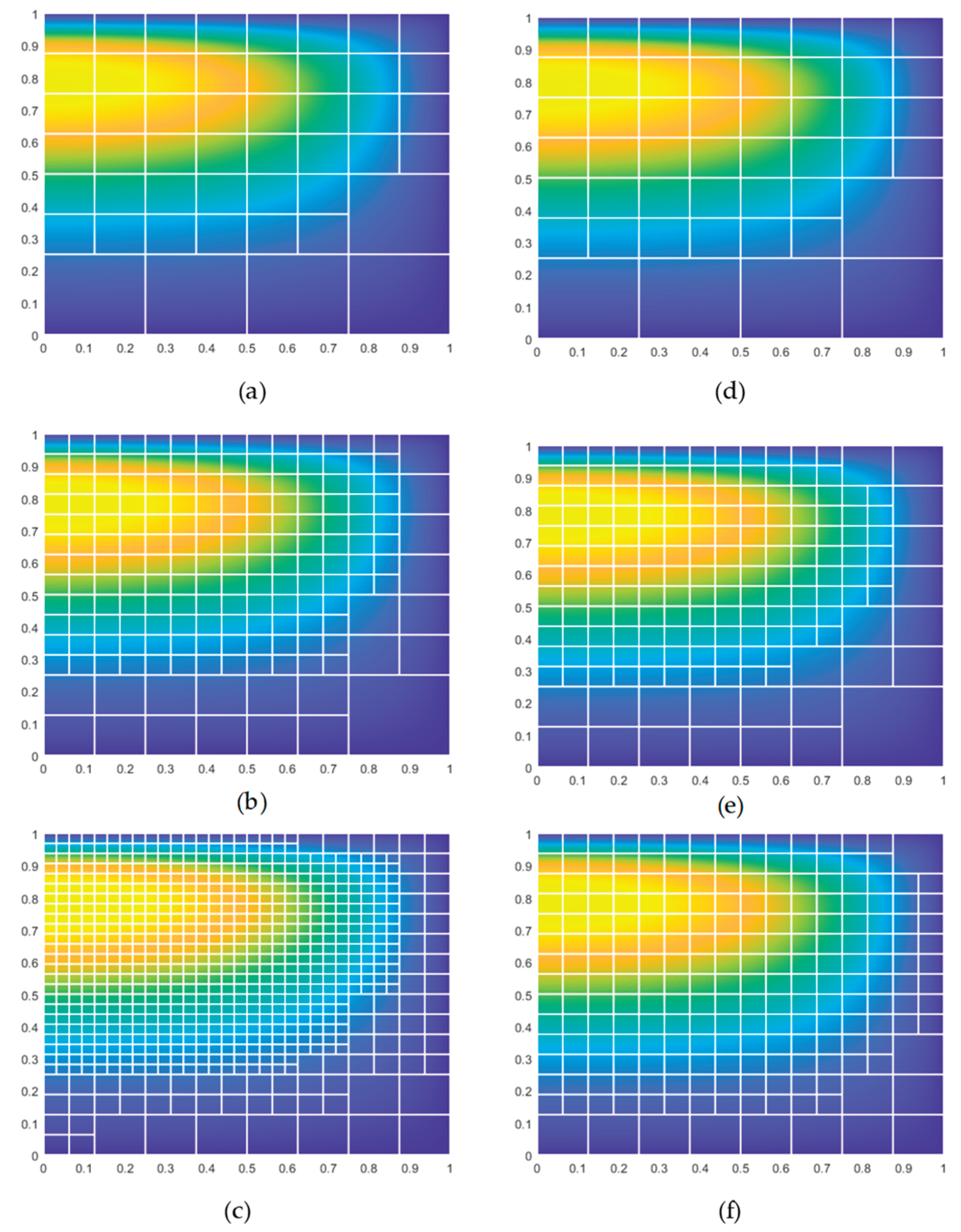
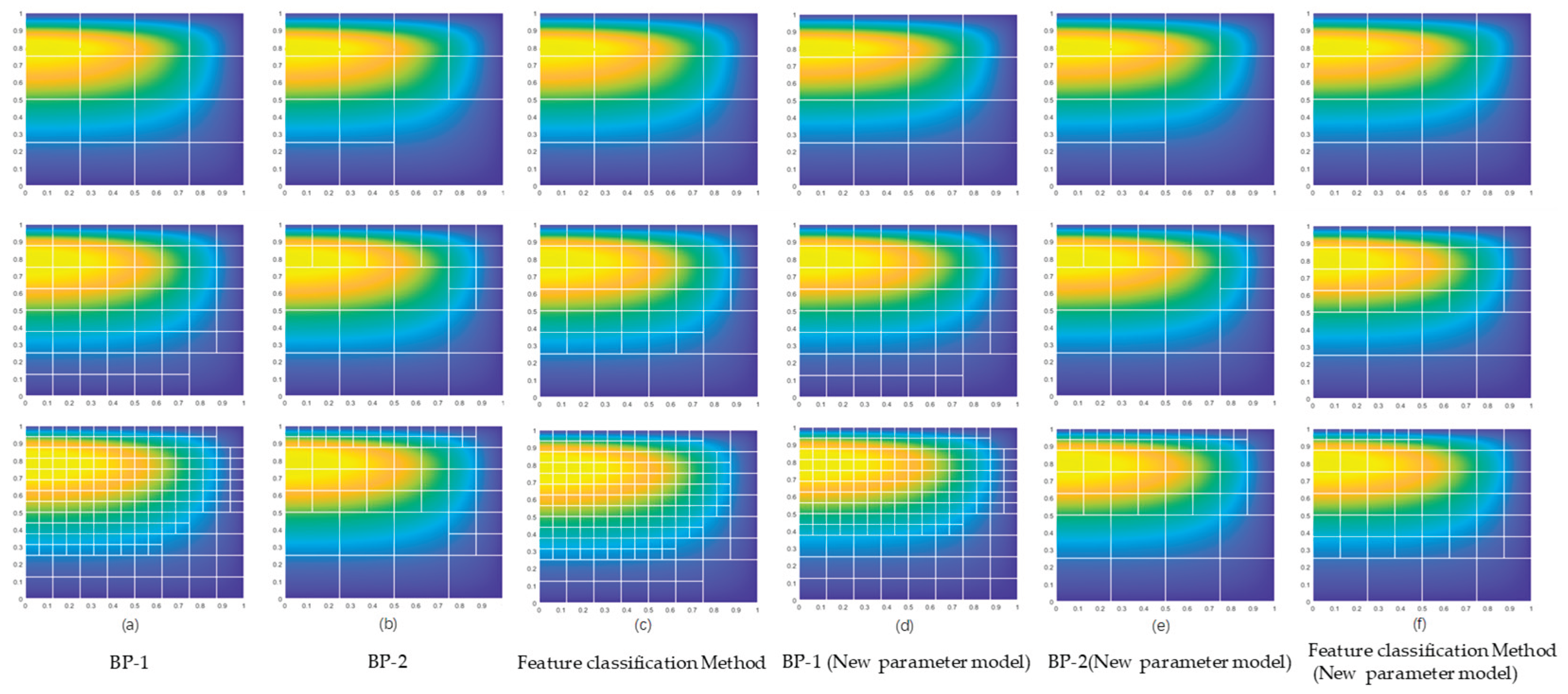
Next, different neural network models can be applied to a unified adaptive refinement algorithm for more specific comparative validation. First, BP-1 and BP-2 are separately integrated into the adaptive refinement algorithm, using four datasets from the hydrostatic sliding bearing model (including new parameters). Additionally, a feature classification method is employed, ultimately generating six refinement results for comparison, as shown in the figure below:
Table 19.
Data Comparison Table for Different Parameter Models and Feature Recognition Methods After Multiple Refinements.
Table 19.
Data Comparison Table for Different Parameter Models and Feature Recognition Methods After Multiple Refinements.
| Refinement method | Number of refinements | Number of elements after refinement | Average prediction accuracy |
| BP-2 | 3 | 46 | 82.97% |
| BP-1 | 3 | 25 | 45.33% |
| Feature classification method | 3 | 44 | - |
| BP-2(NPM) | 3 | 49 | 80.74% |
| BP-1(NPM) | 3 | 25 | 41.33% |
| Feature classification method(NPM) | 3 | 44 | - |
Figure 38.
Comparison of Adaptive Refinement Results Based on Different Parameter Models and Feature Recognition Methods.
Figure 38.
Comparison of Adaptive Refinement Results Based on Different Parameter Models and Feature Recognition Methods.
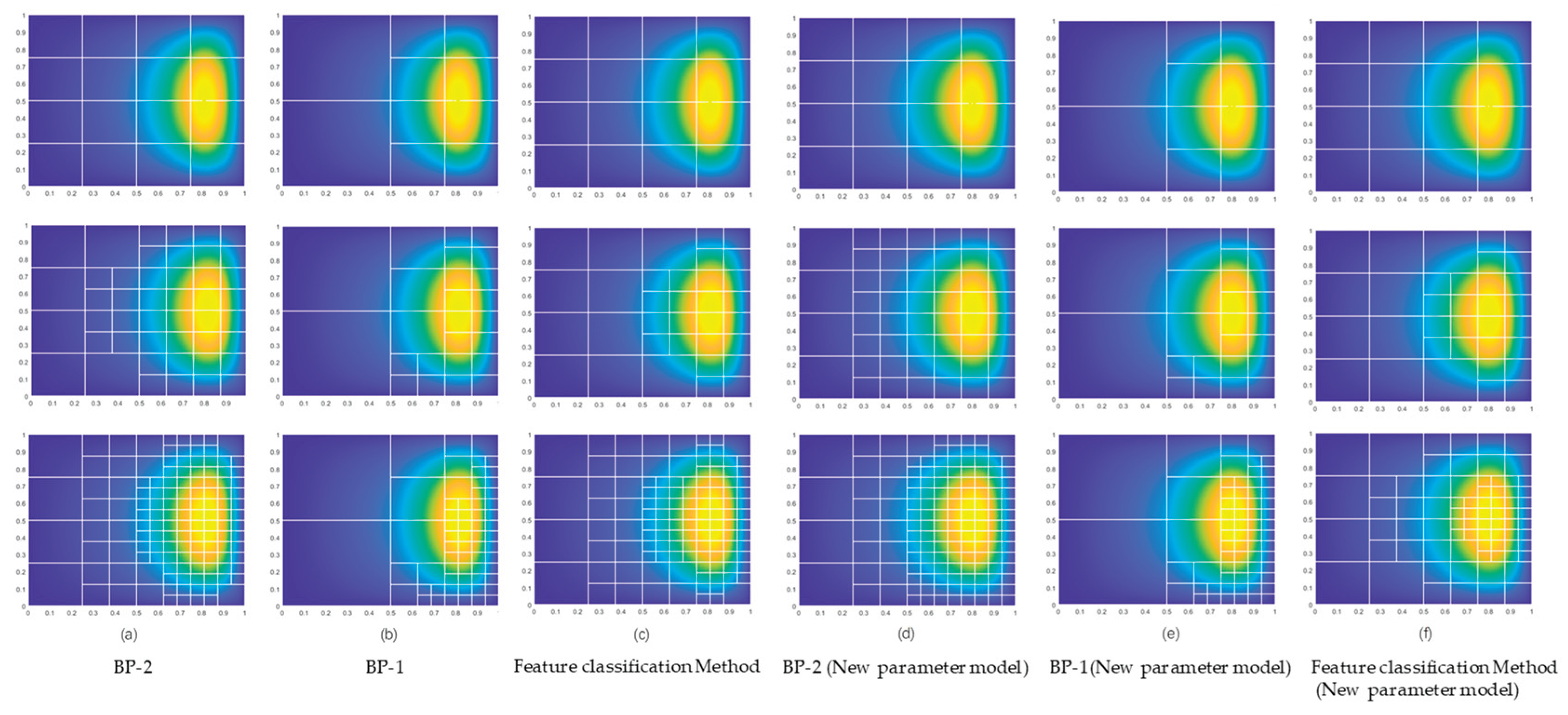
In the table, NPM denotes New Parameters Model. As shown in the comparison figures and tables, BP-2, trained on data from the hydrostatic sliding bearing model, can more accurately predict element categories, thereby achieving superior element refinement performance with a higher average prediction accuracy. Although BP-1, which is unrelated to the training data, is slightly inferior to BP-2 in refinement performance and has lower accuracy, it can still effectively perform feature recognition of critical elements and complete refinement. When the parameters of the hydrostatic sliding bearing model change, both neural networks maintain relatively stable element category prediction capabilities, indicating strong generalization ability.
Subsequently, the lubrication model of the piston-cylinder system was used, with results shown in the figure below:
Figure 39.
Comparison of Adaptive Refinement Results for Lubrication Models Based on Different Parameters and Feature Recognition Methods.
Figure 39.
Comparison of Adaptive Refinement Results for Lubrication Models Based on Different Parameters and Feature Recognition Methods.
By comparing the element refinement results in the figures with Table 20, it is evident that BP-1, trained on its own model data, can better predict the element categories of its own model, while BP-2 performs slightly less effectively but both exhibit stable prediction capabilities. For BP-2, its model demonstrates relatively high prediction accuracy across different lubrication models, indicating superior generalization performance.
Through generalization validation in specific applications, it is confirmed that BP-1 and BP-2 models can handle the refinement process in various lubrication scenarios, although they may underperform compared to specialized models in certain cases. It should be noted that this generalization validation is based solely on the average prediction accuracy of three refinement results, which does not fully reflect the true performance of the BP models. In the future, further model tuning and parameter optimization are expected to significantly enhance the generalization capabilities of BP-1 and BP-2, thereby achieving superior performance and higher robustness in a broader range of application scenarios.
Based on the above concept, BP-3 is similarly applied to both lubrication models, yielding the refinement result figures and performance comparison table as shown below:
Table 21.
Comparison of BP-3 refinement performance across different lubrication models.
| Lubrication model | Number of refinements | Number of elements after refinement | Average prediction accuracy |
| Piston-cylinder system | 3 | 64 | 85.42% |
| Piston-cylinder system (NPM) | 3 | 61 | 76.67% |
| Hydrostatic sliding bearing | 3 | 49 | 80.06% |
| Hydrostatic sliding bearing(NPM) | 3 | 52 | 78.53% |
Figure 40.
Comparison of refinement results for BP-3 applied to different lubrication models.
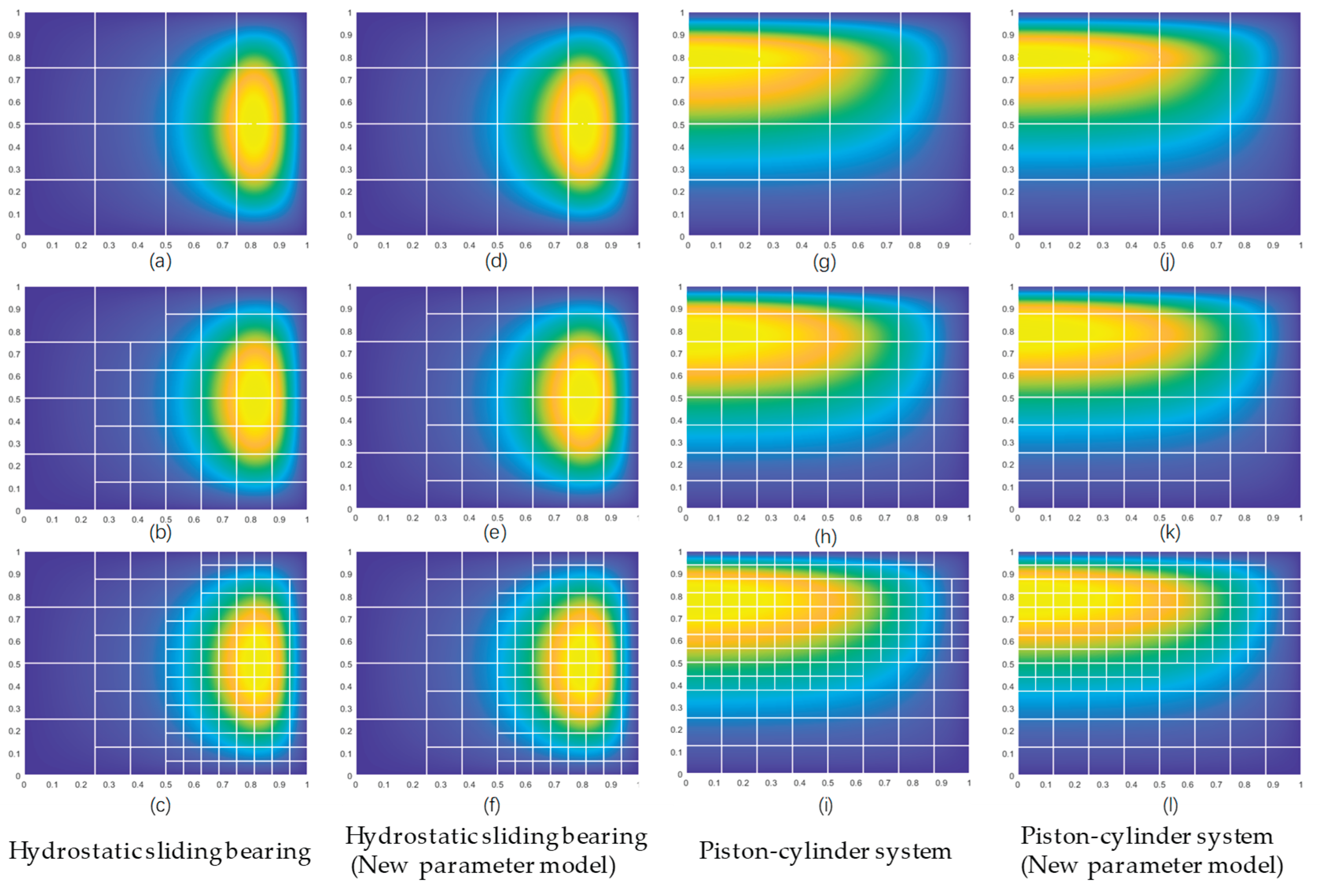
Analysis of the refinement comparison figures and tables reveals that the BP-3 model, trained on mixed data, effectively predicts element categories for both the piston-cylinder lubrication model and the hydrostatic sliding bearing model, achieving a high average prediction accuracy. Additionally, this model demonstrates robust and stable generalization performance, outperforming BP-1 and BP-2 models with notably superior overall performance and prediction accuracy.
Although the feature classification method (Method 2) overcomes many limitations of the residual judgment method based on bubble functions (Method 1) and enhances refinement efficiency through parallel operations in nonlinear transformation and hierarchical clustering, these two steps remain time-consuming when the number of elements is large. In contrast, the BP neural network method (Method 3) eliminates these steps by directly generating outputs from inputs through data parallelism, further improving refinement efficiency. To validate its refinement efficiency, full refinement of elements was performed using the piston-cylinder lubrication model, as shown in the figure below:
Figure 41.
Refinement Result for a Specific Iteration.

Using the element data (16,384 elements) obtained from the sixth full refinement as the data to be predicted, the residual judgment algorithm based on bubble functions (Method 1), the feature classification method (Method 2), and the BP neural network method (Method 3) were applied to classify these data. The time taken is shown in the table below:
Table 22.
Comparison of Time Taken by Three Methods for Element Category Classification.
| Number of samples classified | Time required for Method 1 (s) | Time required for Method 2 (s) | Time required for Method 3 (s) |
| 16348 | 51.234466 | 5.1689 | 0.2423 |
As shown in the table, all three methods classified approximately 16,000 elements. Among them, the BP neural network method required the least time, approximately 1/20 of that needed by the feature classification method, and was even faster than the residual judgment algorithm based on bubble functions.
Overall, within the current research framework, BP-3 enables data parallel operations, efficiently predicting element categories under large element datasets. As a highly efficient neural network model, it relies solely on a single model to effectively handle refinement processes across different lubrication scenarios.
5. Conclusion
This study employed a neural network model to achieve recognition of element refinement features, enabling adaptive refinement for solving the Reynolds equation within the PHT-based IGA framework. The proposed method introduced the concept of refinement features, which incorporated key physical quantities in lubrication analysis, such as pressure and its gradient, alongside element scale from traditional finite element methods, to facilitate global feature recognition and element refinement.
The method proposed in this study has demonstrated the following key advantages: First, it addressed the essential requirements of lubrication analysis by using physical information for the recognition and marking of critical regions. Second, it overcame the limitation of traditional refinement algorithms, which were confined to individual elements, by holistically evaluating refinement regions from the perspective of the solution domain and adaptively adjusting refinement strategies to meet the specific needs of different problems. Third, unlike conventional threshold-based methods, the incorporation of refinement features, combined with data processing techniques commonly used in machine learning, eliminated threshold constraints, achieving strong generalization performance and enabling effective adaptation to the refinement processes of various lubrication problems without requiring specialized data preparation or model training. Finally, the classification and prediction capabilities of machine learning are highly parallelizable, supporting data parallelism, model parallelism, and operation-level parallelism with numerous implementations, thus providing significant efficiency advantages in large-scale applications.
Admittedly, this study has certain limitations. First, the cavitation issue in lubrication problems has not been investigated, which will be a key focus of our future research. Cavitation could serve as a refinement feature, and its corresponding regions should be clearly refined to obtain a reliable oil film pressure distribution. Second, the impact of different classification prediction models and data processing methods on prediction performance has not been thoroughly analyzed. Additionally, while the proposed method achieved good accuracy in the refinement process, it lacks a complete mathematical proof, requiring further validation and refinement.
References
- Patir, N.; Cheng, H.S. An Average Flow Model for Determining Effects of Three-Dimensional Roughness on Partial Hydrodynamic Lubrication. Journal of Lubrication Technology 1978, 100, 12–17. [Google Scholar] [CrossRef]
- Wang, Y.; Wu, J.H.; Xu, L. Influence of power-law fluid on transient performance of liquid film seal based on the time-dependent non-Newtonian dynamic Reynolds equation. Tribology International 2021, 159. [Google Scholar] [CrossRef]
- Yu, X.; Lin, Y.; Wang, P.; Yang, X.; Lan, Z.; Shao, M.; Li, L.; Li, E.; Dai, R.; Jia, W. , et al. Analysis of lubrication characteristics of dynamic-static pressure hybrid thrust bearing considering key factors under eccentric loads. Tribology International 2024, 194, 109471. [Google Scholar] [CrossRef]
- Liu, S.; Gao, L.; Xing, M.; Cui, Y.; Meng, X. A new 3-D multi-physics coupling model for lubricated piston-liner systems. International Journal of Mechanical Sciences 2024, 272, 109194. [Google Scholar] [CrossRef]
- Cai, L.; Wang, Y.; Liu, Z.; Cheng, Q. Carrying capacity analysis and optimizing of hydrostatic slider bearings under inertial force and vibration impact using finite difference method (FDM). Journal of Vibroengineering 2015, 17, 2781–2794. [Google Scholar]
- Zloto, T.; Nagorka, A. An efficient FEM for pressure analysis of oil film in a piston pump. Applied Mathematics and Mechanics 2009, 30, 49–61. [Google Scholar] [CrossRef]
- Arghir, M.; Alsayed, A.; Nicolas, D. The finite volume solution of the Reynolds equation of lubrication with film discontinuities. International Journal of Mechanical Sciences 2002, 44, 2119–2132. [Google Scholar] [CrossRef]
- Liu, C.; Pei, S.Y.; Li, B.T.; Liu, H.L.; Hong, J. NURBS-based IGA of viscous fluid movement with special-shaped small gaps in hybrid bearing. Applied Mathematical Modelling 2022, 109, 401–425. [Google Scholar] [CrossRef]
- van der Meer, G.H.G.; van Ostayen, R.A.J. Efficient solution method for the Reynolds equation with Herschel–Bulkley fluids. Tribology International 2025, 204, 110460. [Google Scholar] [CrossRef]
- Zhang, X.; Xu, X. A moving finite element method for solving two-dimensional coupled Burgers’ equations at high Reynolds numbers. Applied Mathematics Letters 2022, 133, 108271. [Google Scholar] [CrossRef]
- Yang, H.; Zuo, B.; Wei, Z.; Luo, H.; Fei, J. Geometric Multigrid Method for Isogeometric Analysis. CMES - Computer Modeling in Engineering and Sciences 2020, 126, 1033–1052. [Google Scholar] [CrossRef]
- Xu, J.; Xiao, S.; Xu, G.; Gu, R. Parameterization Transfer for a Planar Computational Domain in Isogeometric Analysis. CMES - Computer Modeling in Engineering and Sciences 2023, 137, 1957–1973. [Google Scholar] [CrossRef]
- Yuan, X.; Ma, W. Mapped B-spline basis functions for shape design and isogeometric analysis over an arbitrary parameterization. Computer Methods in Applied Mechanics and Engineering 2014, 269, 87–107. [Google Scholar] [CrossRef]
- Tagliabue, A.; Dedè, L.; Quarteroni, A. Isogeometric Analysis and error estimates for high order partial differential equations in fluid dynamics. Computers & Fluids 2014, 102, 277–303. [Google Scholar] [CrossRef]
- Zhou, W.; Wang, Y.; Wu, G.; Gao, B.; Zhang, W. Research on the lubricated characteristics of journal bearing based on finite element method and mixed method. Ain Shams Engineering Journal 2022, 13, 101638. [Google Scholar] [CrossRef]
- Yan, S.-l.; Zhang, X.-b.; Luo, Z.-h. Adaptive mesh refinement for VOF modeling gas-liquid two-phase flow: A summary of some algorithms and applications. Chemical Engineering Science 2025, 306, 121291. [Google Scholar] [CrossRef]
- Koliesnikova, D.; Ramière, I.; Lebon, F. Fully automatic multigrid adaptive mesh refinement strategy with controlled accuracy for nonlinear quasi-static problems. Computer Methods in Applied Mechanics and Engineering 2022, 400, 115505. [Google Scholar] [CrossRef]
- Kim, B.S.; Kim, K.Y.; Kim, S. Image reconstruction using adaptive mesh refinement based on adaptive thresholding in electrical impedance tomography. Nuclear Engineering and Design 2014, 270, 421–426. [Google Scholar] [CrossRef]
- Cheng, F.; Yu, H.; Wang, Q.; Huang, H.; Xu, W.; Wu, H. Global-local adaptive meshing method for phase-field fracture modeling. Computer Methods in Applied Mechanics and Engineering 2025, 438, 117846. [Google Scholar] [CrossRef]
- Sukas, H.; Sahin, M. A robust monolithic nonlinear Newton method for the compressible Reynolds averaged Navier–Stokes Equations. Computers & Fluids 2025, 289, 106549. [Google Scholar] [CrossRef]
- Hauke, G.; Irisarri, D. A review of VMS a posteriori error estimation with emphasis in fluid mechanics. Computer Methods in Applied Mechanics and Engineering 2023, 417, 116341. [Google Scholar] [CrossRef]
- Venditti, D.A.; Darmofal, D.L. Adjoint Error Estimation and Grid Adaptation for Functional Outputs: Application to Quasi-One-Dimensional Flow. Journal of Computational Physics 2000, 164, 204–227. [Google Scholar] [CrossRef]
- Fidkowski, K.J. Output-based error estimation and mesh adaptation for unsteady turbulent flow simulations. Computer Methods in Applied Mechanics and Engineering 2022, 399, 115322. [Google Scholar] [CrossRef]
- Yuan, H.; Wu, Y.; Zhang, J.; Zhou, S.; Lu, X.; Zhang, Y. Integrated optimization of a turbine stage at a low Reynolds number via NURBS surface and machine learning. Energy 2024, 294, 130956. [Google Scholar] [CrossRef]
- Bazilevs, Y.; Calo, V.M.; Cottrell, J.A.; Evans, J.A.; Hughes, T.J.R.; Lipton, S.; Scott, M.A.; Sederberg, T.W. Isogeometric analysis using T-splines. Computer Methods in Applied Mechanics and Engineering 2010, 199, 229–263. [Google Scholar] [CrossRef]
- Wen, Z.; Pan, Q.; Zhai, X.; Kang, H.; Chen, F. Adaptive isogeometric topology optimization of shell structures based on PHT-splines. Computers & Structures 2024, 305. [Google Scholar] [CrossRef]
- Karuthedath, P.L.; Gupta, A.; Mamindlapelly, B.; Chowdhury, R. A continuous field adaptive mesh refinement algorithm for isogeometric topology optimization using PHT-Splines. Computer Methods in Applied Mechanics and Engineering 2023, 412, 116075. [Google Scholar] [CrossRef]
- Miao, Z.; Chen, Y. VC-PINN: Variable coefficient physics-informed neural network for forward and inverse problems of PDEs with variable coefficient. Physica D: Nonlinear Phenomena 2023, 456, 133945. [Google Scholar] [CrossRef]
- Zou, H.; Zeng, S.; Li, C.; Ji, J. A survey of machine learning and evolutionary computation for antenna modeling and optimization: Methods and challenges. Engineering Applications of Artificial Intelligence 2024, 138. [Google Scholar] [CrossRef]
- Lu, J.; Huang, X.; Li, C.; Xin, R.; Zhang, S.; Emam, M. Multi-Stage-Based Siamese Neural Network for Seal Image Recognition. CMES - Computer Modeling in Engineering and Sciences 2024, 142, 405–423. [Google Scholar] [CrossRef]
- Stock, A.; Moureau, V. Feature-based adaptive mesh refinement for multi-regime reactive flows. Proceedings of the Combustion Institute 2024, 40, 105488. [Google Scholar] [CrossRef]
- Babic, B.; Nesic, N.; Miljkovic, Z. A review of automated feature recognition with rule-based pattern recognition. Computers in Industry 2008, 59, 321–337. [Google Scholar] [CrossRef]
- Kim, Y.-S.; Kim, M.K.; Fu, N.; Liu, J.; Wang, J.; Srebric, J. Investigating the impact of data normalization methods on predicting electricity consumption in a building using different artificial neural network models. Sustainable Cities and Society 2025, 118, 105570. [Google Scholar] [CrossRef]
- Langer, S. Approximating smooth functions by deep neural networks with sigmoid activation function. Journal of Multivariate Analysis 2021, 182. [Google Scholar] [CrossRef]
- Patir, N.; Cheng, H.S. Application of Average Flow Model to Lubrication Between Rough Sliding Surfaces. Journal of Lubrication Technology 1979, 101, 220–229. [Google Scholar] [CrossRef]
- Peiran, Y.; Shizhu, W. A Generalized Reynolds Equation for Non-Newtonian Thermal Elastohydrodynamic Lubrication. Journal of Tribology 1990, 112, 631–636. [Google Scholar] [CrossRef]
- Priest, M.; Taylor, R.I.; Dowson, D.; Taylor, C.M. Boundary Conditions for Reynolds Equation with Particular Reference to Piston Ring Lubrication. In Tribology Series, Dowson, D.; Taylor, C.M.; Childs, T.H.C.; Dalmaz, G.; Berthier, Y.; Flamand, L.; Georges, J.M.; Lubrecht, A.A., Eds. Elsevier: 1996; Vol. 31, pp 441-452.
- Liu, W.; Huang, Z.; Liu, Q.; Zeng, J. An isogeometric analysis approach for solving the Reynolds equation in lubricated piston dynamics. Tribology International 2016, 103, 149–166. [Google Scholar] [CrossRef]
- Yu, D.; Zhu, L.; Shen, H.; Tang, G.; Hu, W.; Dong, F. Classification method of surface defects of silicon nitride bearing rollers based on the coupling of convolutional neural network and dual-kernel support vector machine. Materials Today Communications 2025, 42. [Google Scholar] [CrossRef]
Figure 3.
Illustration of relative scale.

Figure 17.
Flowchart of the Neural Network-Based Feature Recognition Process.
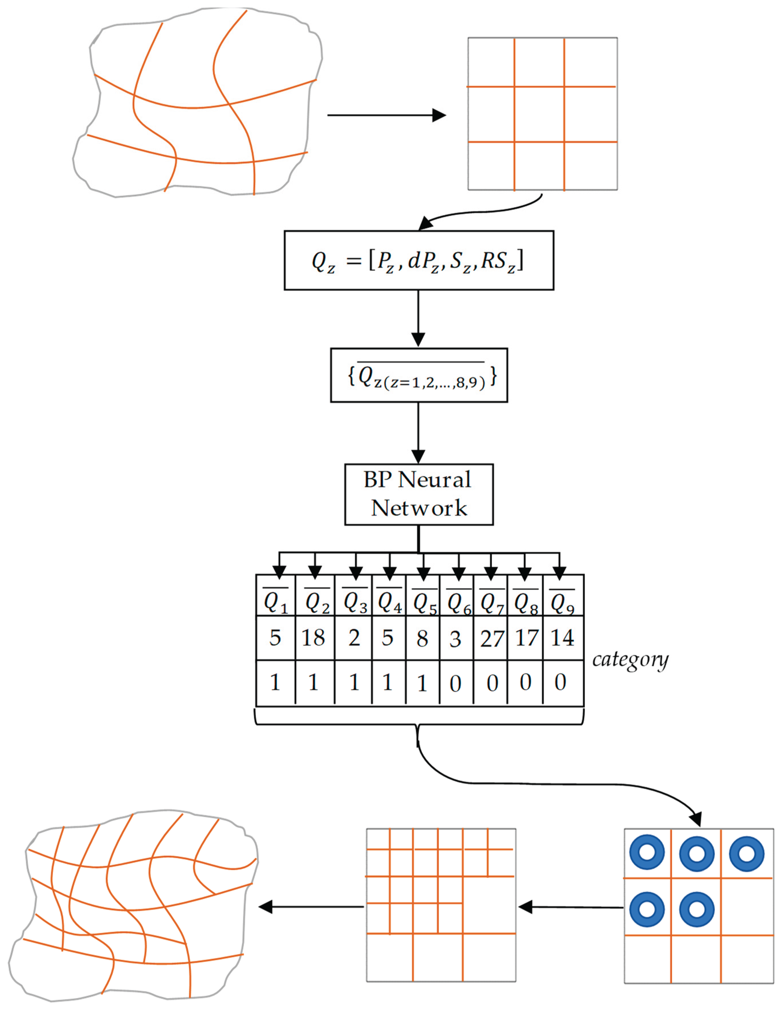
Figure 18.
Refinement Results of the Feature Recognition Algorithm Based on Neural Networks.
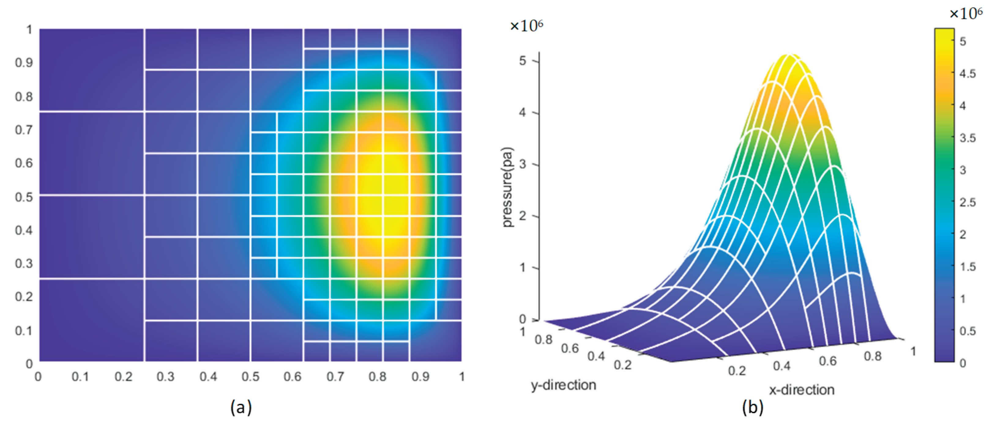
Figure 19.
Refinement Results Based on Feature classification.
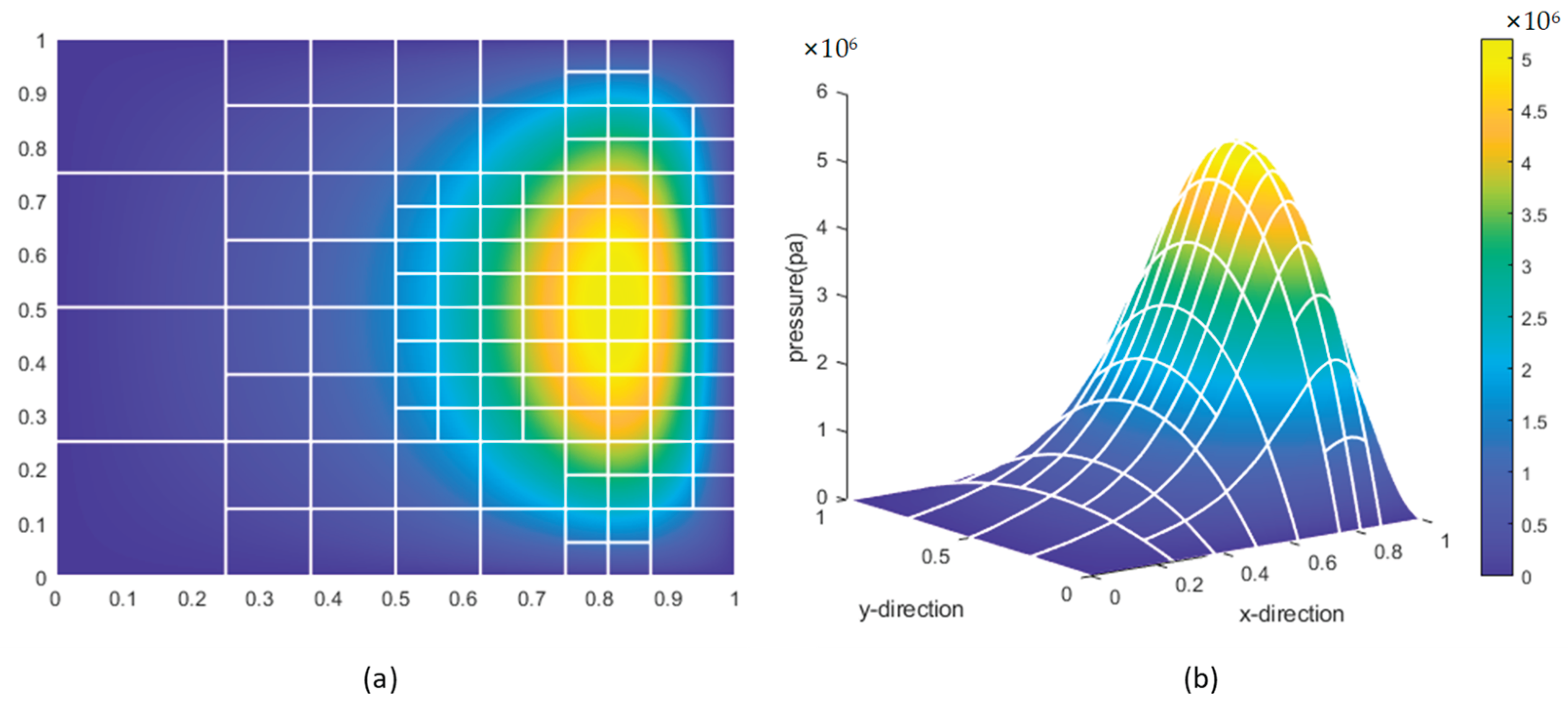
Figure 20.
Complete Refinement Process of the Feature Recognition Algorithm Based on Neural Networks.
Figure 20.
Complete Refinement Process of the Feature Recognition Algorithm Based on Neural Networks.

Figure 27.
Comparison of refinement results using feature classification-based and local consideration PHT-IGA methods.
Figure 27.
Comparison of refinement results using feature classification-based and local consideration PHT-IGA methods.
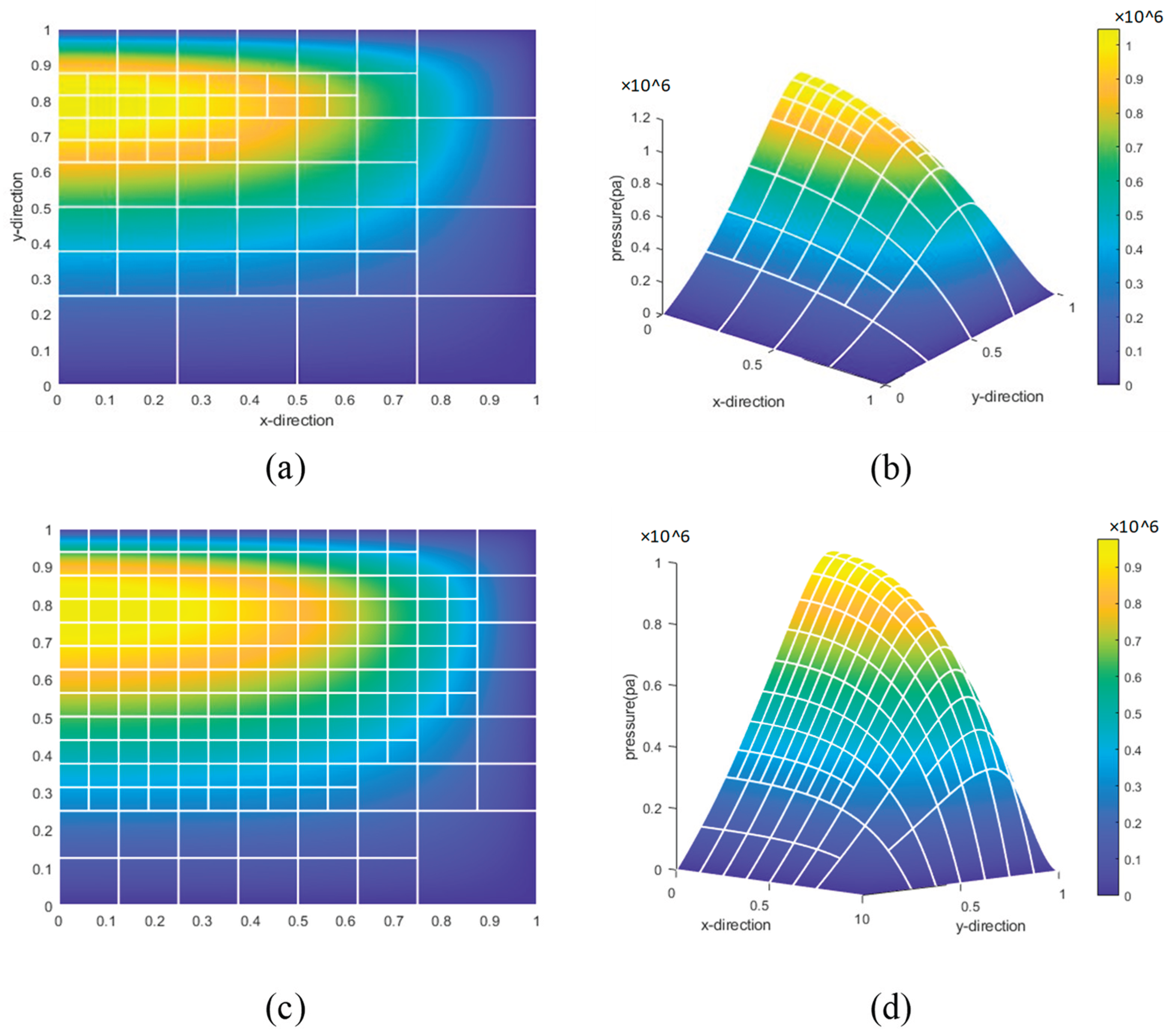
Figure 30.
Residual Distribution of Different SVM Models.
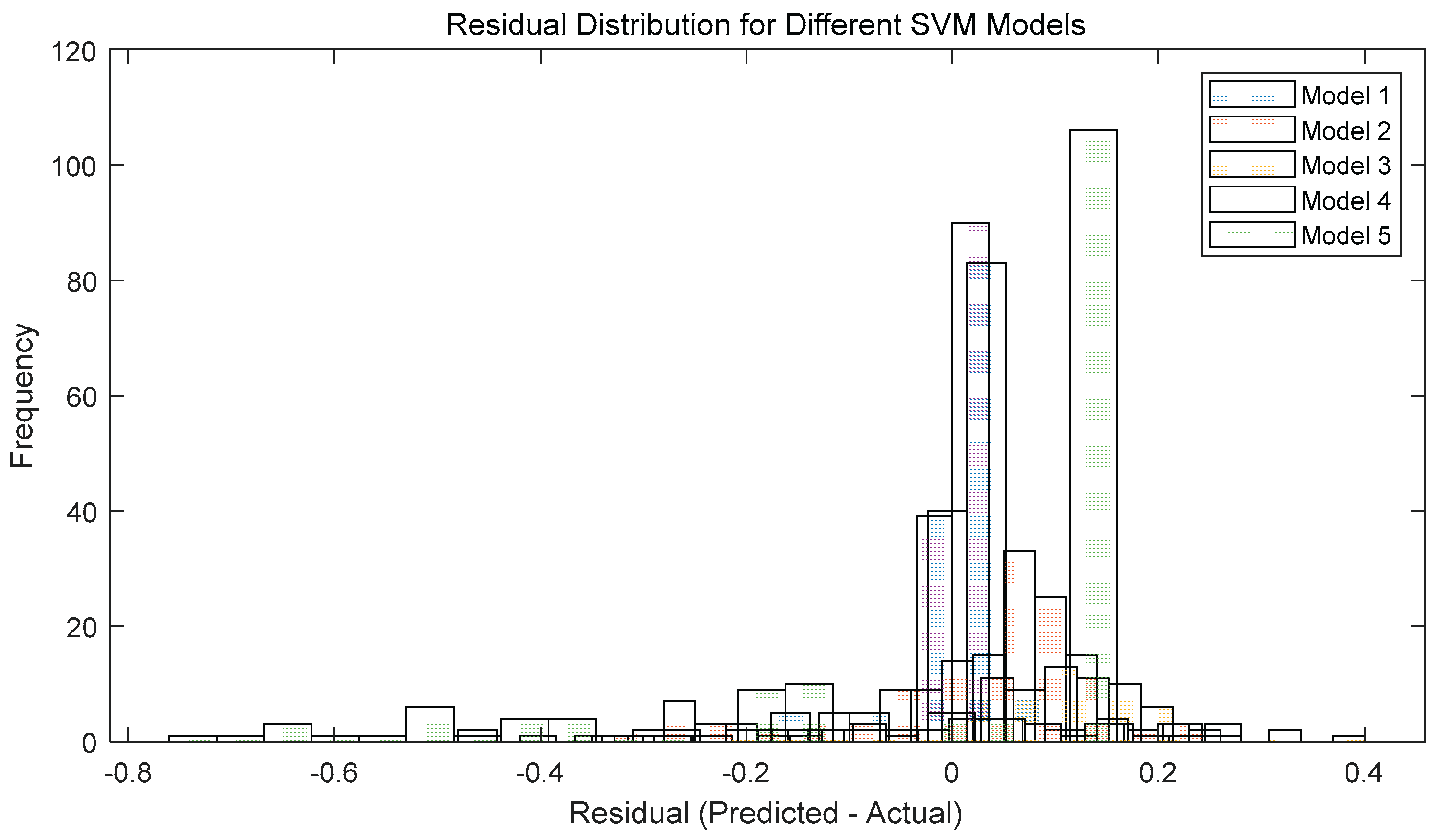
Figure 31.
Output Accuracy of SVM Models with Different Parameters.
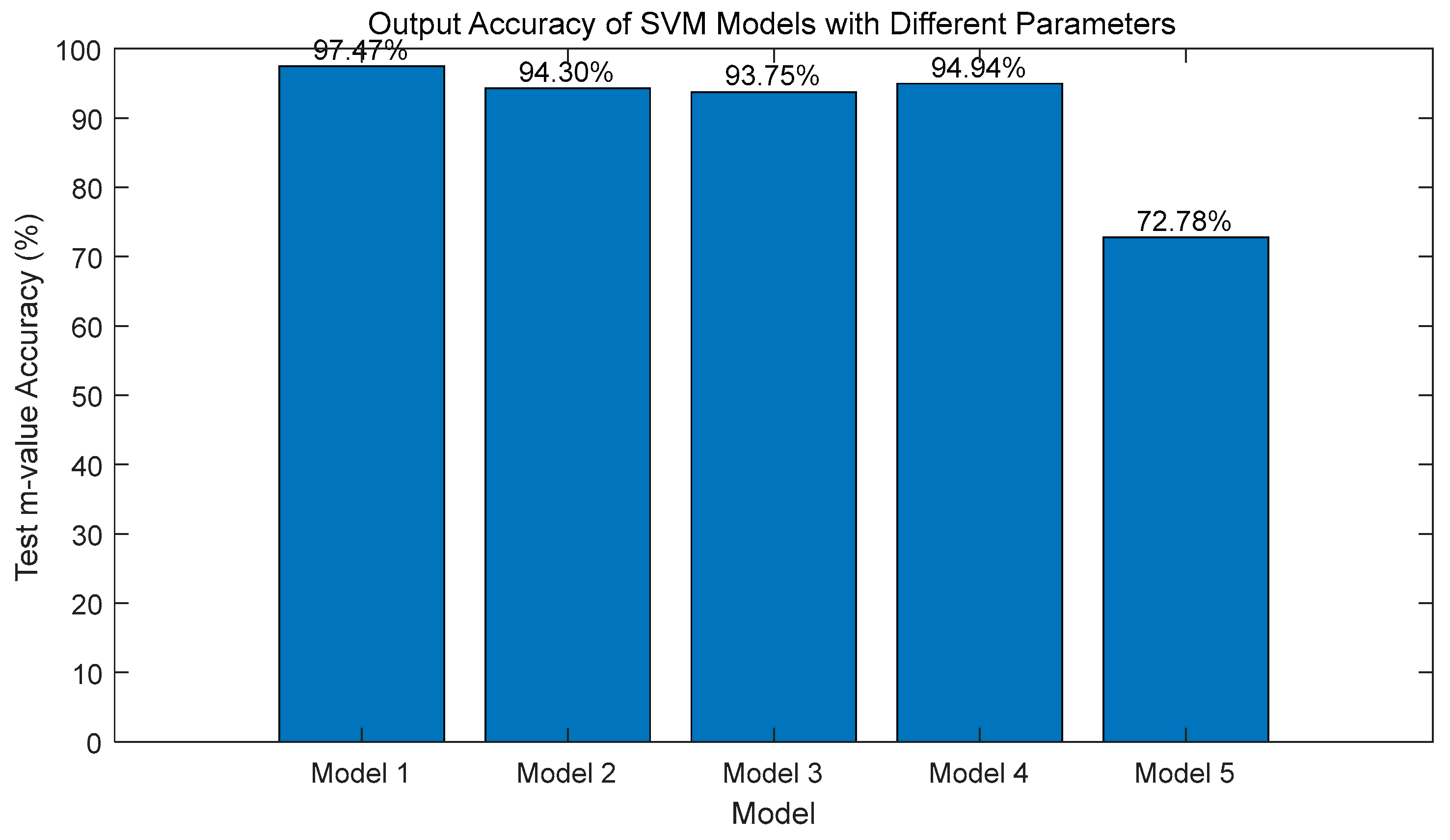
Figure 32.
Refinement Results of Feature Recognition Methods Based on Neural Network and Support Vector Machine (SVM).
Figure 32.
Refinement Results of Feature Recognition Methods Based on Neural Network and Support Vector Machine (SVM).
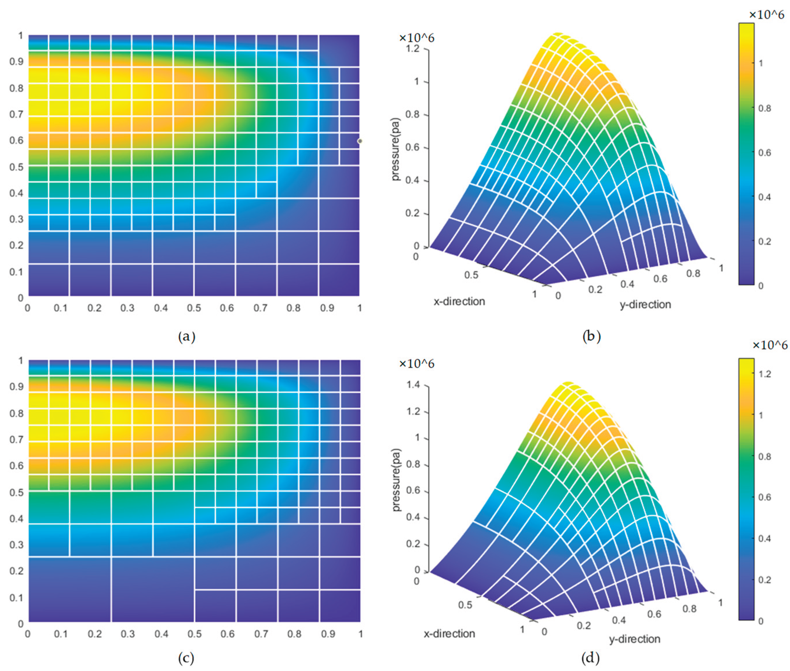
Figure 33.
Schematic diagram of the lubrication model for a radial bearing.
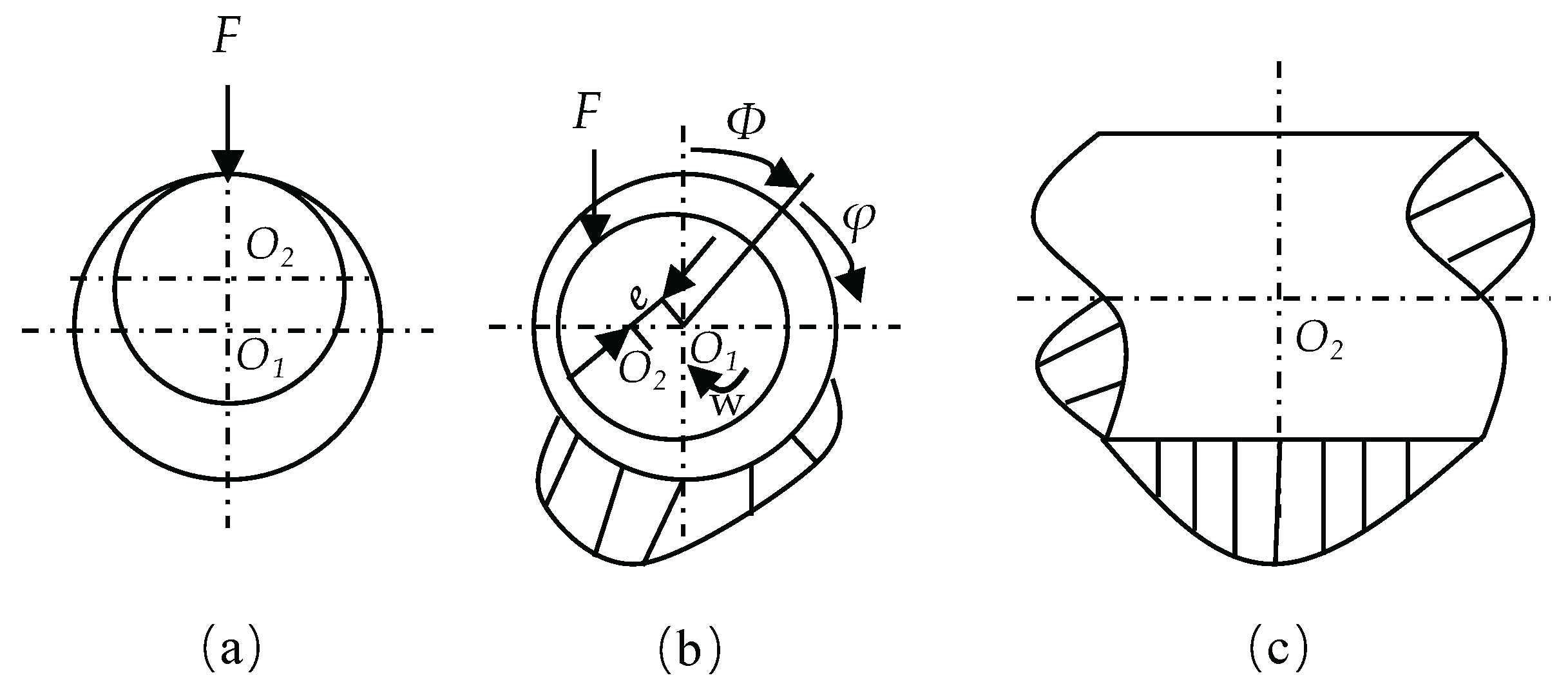
Table 9.
Basic input parameters in the calculation example.
| Parameter | Description | Worth | Element |
| Piston skirt radius | |||
| Cylinder liner radius | |||
| Piston skirt length | |||
| Lubricating oil viscosity | |||
| Eccentricity of the upper end of the piston skirt | |||
| Eccentricity of the lower end of the piston skirt | |||
| Derivative of with respect to time | |||
| Derivative of with respect to time | |||
| Piston reciprocating speed | |||
| Vertical distance from piston pin to top of piston | |||
| Distance from piston pin to piston centerline |
Table 12.
New Parameters for the Piston-Cylinder System Model.
| Parameter | Description | Worth | Element |
| Piston skirt radius | |||
| Cylinder liner radius | |||
| Piston skirt length | |||
| Lubricating oil viscosity |
Table 20.
Data Comparison Table for Lubrication Models Based on Different Parameter Models and Feature Recognition Methods After Multiple Refinements.
Table 20.
Data Comparison Table for Lubrication Models Based on Different Parameter Models and Feature Recognition Methods After Multiple Refinements.
| Refinement method | Number of refinements | Number of elements after refinement | Average prediction accuracy |
| BP-1 | 3 | 61 | 81.28% |
| BP-2 | 3 | 31 | 71.98% |
| Feature classification method | 3 | 64 | - |
| BP-1(NPM) | 3 | 61 | 75.03% |
| BP-2(NPM) | 3 | 31 | 74.55% |
| Feature classification method(NPM) | 3 | 52 | - |
Disclaimer/Publisher’s Note: The statements, opinions and data contained in all publications are solely those of the individual author(s) and contributor(s) and not of MDPI and/or the editor(s). MDPI and/or the editor(s) disclaim responsibility for any injury to people or property resulting from any ideas, methods, instructions or products referred to in the content. |
© 2025 by the authors. Licensee MDPI, Basel, Switzerland. This article is an open access article distributed under the terms and conditions of the Creative Commons Attribution (CC BY) license (http://creativecommons.org/licenses/by/4.0/).
Copyright: This open access article is published under a Creative Commons CC BY 4.0 license, which permit the free download, distribution, and reuse, provided that the author and preprint are cited in any reuse.


