Submitted:
06 June 2025
Posted:
09 June 2025
You are already at the latest version
Abstract
Computer vision is a critical artificial intelligence component that enables machines to interpret and make decisions based on visual data. As we move towards an era where machines are increasingly responsible for decision-making, vision becomes a fundamental sensory modality for machines to perceive and understand their environment. The ability of machines to "see" and comprehend the world through visual input raises the question of whether they can truly grasp complex situations based on the objects and interactions within their surroundings. This paper provides a comprehensive exploration of the core concepts and algorithms underlying computer vision, starting from its early stages of development. It delves into foundational techniques, discussing their evolution and innovations shaping the field. Additionally, the paper addresses the inherent limitations of these foundational concepts and explores how they have influenced the development of current technologies. A critical analysis of present-day technologies is also provided, highlighting their challenges and limitations despite significant advances. Finally, the paper explores the wide-ranging applications of machine vision across various domains and the promising future prospects for the continued advancement of computer vision technologies.
Keywords:
Computer Vision
; Deep Learning
; Machine Learning
; Artificial Intelligence
1. Introduction
What is artificial intelligence (AI)? To understand AI, we first need to know what intelligence is. In short, we can say that intelligence is to make a beneficial decision by perceiving the environment [1]. The human brain is naturally born intelligent, and human can learn from their decision while growing up. Artificial is what humans create and not natural. Artificial Intelligence stands for a created model or machine that can make decisions based on the environment and objects in the environment [2]. Can machines think? This question was asked by Alan Turing [3] when he tried to find if the machine could think. Machines may not think automatically, but they can make beneficial decisions based on the environment and rewards. We have come a long way from that. Nowadays, machines can recognize patterns and images and make decisions. But can we tell that machines have already gained intelligence like humans? Human decision-making is a very complex and arguable subject. Still, a decision is usually made by observing the environment and based on the objects they find around or the senses humans get by interacting with other objects. Humans have many senses, but one of the most important is vision [4]. By vision or observation, humans develop their brains by making decisions and learning. Computer vision was created by looking through cameras based on human vision. The early development of computer vision [5] was not far from now. Still, it is a subject of improvement. It is an essential and very important part of the decision-making approach of a machine. Vision is a sense that can visualize the objects of the environment by the reflection of light [6]. Human eyes see objects when light reflects off objects. Without lights or a very small amount of reflection, the human eye loses its ability to visualize objects. Computer vision trains machines to perform object identification, distance, and movement using cameras, data, and algorithms instead of retinas, optic nerves, and the visual cortex. This system can analyze thousands of products or processes per minute, surpassing human capabilities. Computer vision began in the late 1960s to mimic the human visual system and enable robots to behave intelligently. It aimed to extract three-dimensional structures from images for full scene understanding. Early studies in the 1970s formed the foundations for many computer vision algorithms today. The next decade saw more rigorous mathematical analysis and quantitative aspects of computer vision, such as scale-space, shape inference, and contour models. By the 1990s [5], research focused on projective 3-D reconstructions, camera calibration, sparse 3-D reconstructions, dense stereo correspondence, and image segmentation. The field of computer graphics and computer vision also increased, leading to the resurgence of feature-based methods and the advancement of deep learning techniques. Computer vision is a crucial tool in various fields, including medicine[7,8], industry[9], military[10], and autonomous vehicles[11,12]. In medicine, it is used for diagnosing patients, enhancing images interpreted by humans, and supporting research. In industry, it is used for quality control, inspection of final products, and agricultural processes. In military applications, it is used for detecting enemy soldiers or vehicles and for missile guidance. Advanced systems use image data to target specific areas, reducing complexity and increasing reliability. Autonomous vehicles, including submersibles, land-based vehicles, aerial vehicles, and unmanned aerial vehicles (UAV), use computer vision for navigation, obstacle detection, and task-specific events. Computer vision is a vital tool in various fields, including medicine, industry, and space exploration. This paper explores the core concepts of computer vision, key algorithms, and recent advancements in the field. Additionally, it examines future trends and addresses ethical considerations. The discussion section highlights current computer vision methods’ limitations and provides insights into future research directions.
2. Computer Vision: Enabling Visual Perception in Machines
A computer system uses visual data to recognize objects, such as a cat image. The image is preprocessed and analyzed for details like edges, shapes, or colors. The system then trains the model using thousands of positive and negative cat pictures to learn unique patterns. The system then classifies the object in a new image based on the learned patterns, predicting its classification. The system outputs the result by highlighting the cat or labeling it as a cat. To analyze the image, the system first needs to know what an image is. An image is like a grid of tiny squares (pixels); each square has a color or shade. For black-and-white images, the squares are either black or white. For grayscale images, each square is a shade of gray, ranging from black to white. Each square has a mix of three colors for color images: red, green, and blue (RGB) [13]. In short, we can say that an image is a 2-dimensional function , where x and y are spatial (plane) coordinates, and h represents the amplitude (e.g., intensity or color) at each point. There are two types: analog images, represented as continuous real numbers, and digital images, defined as discrete integers with quantized amplitude values, such as digital photographs and bitmap graphics. Computer vision processes digital images using an algorithm. Digital image processing involves processing digital images using a digital computer. These images consist of finite elements, known as picture elements, image elements, pels, or pixels, with pixels being the most commonly used term. Its data needs to be converted into digital data to process the analog images. Figure 1 explains an image with the original image, its 2D visualization of grayscale image 3D visualization of intensity, and the matrix of pixel values of the digital image.
Computerized processes can be classified as low-, mid-, or high-level [14]. Low-level processes involve image preprocessing, which reduces noise and enhances contrast. Mid-level processes involve segmentation, description, and classification of objects. High-level processing makes sense of an ensemble of recognized objects and performs cognitive functions associated with vision. Examples include automated text analysis, which involves acquiring an image, preprocessing it, extracting individual characters, describing them, and recognizing them. Digital image processing encompasses these processes.
2.1. Foundational Techniques
Computer Vision is built on mathematical concepts and algorithms that process and interpret visual data. Below are some foundational techniques, their mathematical principles, and examples.
2.1.1. Edge Detection
Edges are the lines where colors or brightness change sharply in an image, like the outline of a building against the sky. Detecting these edges helps computers understand the shapes of objects in an image[15]. For instance, Figure 2 shows the outline of a statue. In this image, it is clear to see the edges of the statue, the edges of the beads, and the edges of the pot put in front of the feet of the statue.
Edge detection identifies regions with high-intensity gradients using:
Where,
In the equation:
- and are partial derivatives of the image function with respect to x and y. These derivatives measure how much the pixel intensity changes along the horizontal direction (x) and the vertical direction (y);
-
Specifically:
- –
- tells us how the image intensity changes as we move left or right.
- –
- tells us how the image intensity changes as we move up or down.
-
Gradient magnitude is computed by combining the horizontal and vertical gradients with this equation:This gives a measure of the overall change in intensity at each point. The higher the value of , the more likely that point is an edge.
- and measure image changes in x and y directions, combining them to calculate intensity at each pixel, aiding in detecting significant brightness or color changes.
2.1.2. HOG (Histogram of Oriented Gradients)
HOG is a feature extraction technique in computer vision to detect objects in images [17]. If there is a photo of a face or human, then this feature captures the shape of objects based on pixel intensities, focusing on edges and contours. The process involves dividing the image into small regions, calculating the gradient in each region, and summarizing these gradients in a histogram. We know there is an edge if the change is large (e.g., from dark to light). In simpler terms, it tells us how quickly the image becomes brighter or darker. There is no edge if the change is small (e.g., from light to slightly darker). The gradient is calculated for each pixel using the Sobel [18] operator or other methods:
Where is the intensity value at the pixel . and represent the horizontal and vertical changes in intensity. Once we have the gradients, we compute the magnitude and orientation of the gradients for each pixel:
In a face photo, HOG would work by calculating the brightness of each pixel, dividing the image into cells, typically 8x8 pixels. Then, compute a histogram of the edge directions in each section. The histogram will have bins corresponding to different angles (e.g., 0°, 45°, 90°, etc.), and each pixel contributes its gradient magnitude to the appropriate bin based on its orientation. To make the descriptor robust to changes in lighting, each cell’s histogram is normalized with respect to its neighboring cells (this is called block normalization). A block typically consists of multiple cells (e.g., 2x2 cells). Figure 3 illustrates the HOG features.
The normalization ensures that variations in lighting don’t affect object detection. Once we have histograms for all the cells and blocks, we combine them into a feature vector. Which is used by a machine learning model like a Support Vector Machine (SVM)[19] to recognize if the image contains a face based on its training data. HOG is helpful for object detection because it captures essential visual features, is robust to changes in lighting and small distortions, and works well in tasks like detecting pedestrians, vehicles, and faces in images or videos.
2.1.3. Feature Extraction
Feature extraction is a key process in computer vision that helps a computer understand and identify objects in an image [20]. Features are unique patterns in an image, like corners, lines, or textures. Computers look for these features to recognize objects. For instance, the corner of a table or the stripes on a zebra are features that help identify them. Please consider how we might recognize a friend by their hairstyle or glasses. These distinctive features stand out and help us to identify them, even in a crowd. Features are critical for object recognition because they help simplify the problem. Instead of comparing every pixel in an image, a computer looks for key features that stand out and give clues about the object. For example, a corner in an image could signify the intersection of two surfaces in a 3D object, or a line might indicate the edge of a shape. One common approach to feature extraction is to use gradient-based methods that detect the change in pixel intensities across an image. A common feature extraction technique is Harris Corner Detection[21], which detects corners in an image. In this method, we calculate a measure R to evaluate the significance of a corner at each point in the image. The equation for Harris corner detection is:
Where:
- M is a 2x2 matrix of image gradients at a particular point in the image.
- refers to the determinant of the matrix M, which provides information about the area’s cornerness.
- is the sum of the diagonal elements of the matrix M, which indicates how much the pixel values change in different directions. A high trace value means there’s a significant intensity change
- k is a sensitivity factor, typically a small constant (e.g., ) that helps adjust the calculation. A smaller k results in more points being detected as corners, while a larger k makes the detection stricter, only identifying strong corners.
- The final value R is used to determine whether a pixel is a corner. A high value of R indicates that the point is a corner, while a lower value suggests the point is not.
The matrix M is built using gradients (changes in pixel intensities) in both the horizontal and vertical directions (often computed using Sobel operators). This matrix helps us capture the direction and magnitude of intensity changes at a specific point.
Where: is the gradient in the x-direction (horizontal), and is the gradient in the y-direction (vertical). Imagine a photograph of a desk with a coffee mug on it. The edges of the mug, where it touches the desk, create corners. The algorithm looks at the gradients around these points to find areas with strong changes in pixel intensity. The sharp line where the desk surface meets the coffee mug is an edge, another feature the computer will detect. The patterns on the desk, like wood grain, also help distinguish the desk from the mug. Using feature extraction methods like Harris Corner Detection, the computer can detect these corners and edges, enabling it to understand the basic layout of the image. Once these features are detected, the computer can match and recognize the objects (the desk and mug) in other images.
2.2. Challenges in Computer Vision
While foundational techniques like edge detection, HOG (Histogram of Oriented Gradients), and feature extraction have been widely used in computer vision, they come with various challenges. These techniques aim to identify key features and structures in images, but real-world applications introduce complexities that make accurate recognition difficult. Below, I will explain some of the challenges associated with these techniques, particularly focusing on occlusion and scalability, which are significant issues in practical scenarios.
2.2.1. Occlusion
Occlusion(Figure 4) refers to when part of an object is hidden or blocked by another object in the scene. This is a common challenge in real-world computer vision tasks, where objects in an image may not be fully visible due to overlap with other objects or elements in the environment.
Occlusion[22] can affect computer vision algorithms by causing incomplete features, misleading gradients, and causing object tracking issues. Incomplete features, such as edges or corners, may be missed or incomplete, making it difficult for the algorithm to recognize the object accurately. Occlusion can also distort gradients, leading to false edge detections. HOG, which detects local gradients and edge orientations, may be incomplete when parts of an object are occluded, making it difficult for the algorithm to recognize the object accurately. In dynamic environments, occlusion can confuse object-tracking algorithms, causing them to lose track of the object. The visibility of a pixel or object can be modeled as a binary mask , where:
When an object is occluded, only the visible parts are captured in the image :
This masking operation leads to partial or missing data in the image. For example:
- In edge detection, gradients in occluded regions may be incomplete or distorted.
- In feature extraction, feature descriptors such as SIFT or HOG rely on the visible region and cannot account for missing parts.
Imagine you are trying to detect a car on a busy street, but other vehicles are blocking parts of the car. The edge detection or HOG features might only capture the visible part of the car, leading to incomplete recognition or misclassification. Occlusion affects object recognition by creating incomplete feature sets. Consider an object O represented by a set of features . When some features are occluded, only a subset is available.
The recognition task then becomes one of matching S to the known feature set under uncertainty:
where represents a known object. The similarity score may drop below the recognition threshold if the occlusion is significant. In HOG, occlusion can disrupt the computation of gradient histograms. If a person’s torso is occluded, gradients in those regions will not contribute to the histogram. Mathematically, if a gradient is part of the occluded region (), it is excluded from the histogram calculation.
2.2.2. Scalability
Scalability[23] refers to the ability of an algorithm to handle images or data that vary in size, resolution, or complexity. It is important for computer vision techniques to work effectively across a wide range of image scales (small images vs large images) and conditions (low resolution vs high resolution). In real-world images, objects can appear at different sizes due to changes in distance or perspective, making feature extraction techniques like HOG difficult to handle. High-resolution images contain more details and require more computational resources, making edge detection algorithms slower or less accurate when applied to high-resolution images. Lower-resolution images may lose important details, making feature extraction less effective. As the size of the image increases, the number of calculations required for edge detection, HOG, or feature extraction increases significantly, leading to high computational costs and slow processing times, especially for real-time applications like video surveillance or autonomous driving. Multi-scale issues also pose a challenge, as some computer vision techniques, like HOG, assume that the object being detected is approximately the same size in the image. Scaling an algorithm to handle various object sizes without losing accuracy is a significant challenge. In real-world images, the same object O can appear at different scales s:
where represents upscaling, and represents downscaling.
When detecting an object at different scales, the feature space extracted from changes with s. Features like edges or keypoints may disappear or change orientation at extreme scales.
To address this, multi-scale processing involves creating an image pyramid:
where represents the image scaled by s. Algorithms then process each level of the pyramid to find scale-invariant features. For an image of size , the computational cost of many vision algorithms increases with the number of pixels . For example:
- Edge Detection: Computing gradients involves operations for each pixel, leading to complexity.
- HOG: Constructing histograms across overlapping blocks increases complexity to approximately , where B is the number of blocks.
-
Feature extraction and matching also need to be scale-invariant. For example, the similarity between two objects O and can be computed using a transformation-invariant distance d:where T is a transformation (e.g., scaling, rotation).Without proper scaling mechanisms, the distance d increases as the object size changes, leading to poor recognition results.
If you try to detect a person in an image, a standard HOG detector may work well when the person is near the camera and occupies a large portion of the image. However, if the person is far away, their features become smaller and less distinct, and the HOG detector may fail to recognize them. Similarly, if the image is very large or of high resolution, the computational requirements to detect the person increase, leading to slower processing times. Figure 5 represents the digital image and its edges.
2.3. Additional Challenges in Foundational Techniques
- Noise sensitivity: Edge detection algorithms like Sobel or Canny are noise-sensitive. In real-world images, noise can lead to false edges being detected or important edges being missed.
- Weak boundaries: Some objects might have weak or fuzzy edges (e.g., transparent objects, low-contrast images), which makes it difficult for traditional edge detection methods to identify them.
- Limited to visible features: HOG works by detecting gradients (changes in intensity). However, objects with less clear edges or softer gradients (like a blurred object or one in shadow) are harder to detect.
- Sensitivity to pose variations: HOG features might be sensitive to the object’s orientation. If the object is rotated or skewed, the feature extraction process might miss important patterns, reducing accuracy.
- Feature mismatches: For complex objects, feature extraction methods may miss or incorrectly identify key features. For example, in an image with a cluttered background, it may be difficult to extract clean features due to the noise from the background.
- Feature diversity: Different objects require different features for recognition. For example, recognizing a dog may require detecting texture features (fur), while recognizing a car may require detecting edges and corners. Designing universal feature extraction methods that can work for all object types is a complex challenge.
Occlusion and scalability pose significant challenges to foundational computer vision techniques like edge detection, HOG, and feature extraction. Occlusion obscures crucial features, making object detection harder. Scalability involves handling images of varying sizes and resolutions, but computational requirements for large images can be challenging.
3. Key algorithms and Advances
Traditional methods, such as SIFT, HOG, and Haar cascades, relied on handcrafted features and explicit programming to solve vision tasks. These methods had several drawbacks, including being task-specific, having difficulty in capturing complex patterns, being slow and impractical for large-scale datasets, being sensitive to noise and variations, and lacking end-to-end learning. Handcrafted features were designed and tailored to specific tasks or datasets, making it difficult to generalize to new data or tasks. They also struggled with complex tasks like object detection or semantic segmentation, where understanding context and relationships is crucial. Scalability issues were also challenging, as manual feature design was slow and impractical for large-scale datasets. Handcrafted features were also sensitive to variations in lighting, rotation, occlusion, and scale, making it challenging to recognize rotated or partially occluded objects. Deep learning-based models were introduced to address the limitations of traditional methods in computer vision and other domains. The development of neural networks began in the 1943-1980s[24] with the foundations laid by McCulloch and Pitts. Rosenblatt developed the perceptron in 1958[25], and the multi-layer perceptron (MLP) was introduced in 1998[26]. Convolutional Neural Networks (CNNs)[27] were introduced in 1998 by Yann LeCun, but faced challenges due to computational power and the vanishing gradient problem. In 2012, AlexNet[28] and ImageNet[29] were introduced, achieving breakthrough performance in the ILSVRC competition. Modern architectures introduced deeper, more efficient networks like VGGNet[30], ResNet[31], Inception[32], and EfficientNet[33], and advancements in object detection and segmentation. In 2021, Vision Transformers (ViTs)[34] and Generative AI[35] were adopted for computer vision tasks. Deep learning[36] is a powerful tool that automates feature extraction by learning relevant features directly from data and optimizing them according to the task objective. It can model complex data with high dimensionality, allowing deep neural networks to understand low-level features in shallow layers and combine them into high-level representations in deeper layers. Pretrained deep learning models can be fine-tuned for diverse tasks, reducing the need for task-specific feature engineering. Deep learning is particularly well-suited for large datasets, such as ImageNet, where data abundance is common. For instance, deep learning models like AlexNet outperformed traditional methods significantly on ImageNet, a dataset with millions of labeled images. Advances in hardware and algorithms, such as GPUs and TPUs, have enabled faster training of deep models, with techniques like backpropagation, ReLU activation, dropout, and batch normalization improving training stability and performance. Deep learning represents a paradigm shift in computer vision, moving away from manual intervention and toward models that learn directly from data. It capitalizes on advances in data availability, hardware, and algorithms, offering solutions to problems that traditional methods could not address effectively.
3.1. Convolutional Neural Networks (CNNs)
CNNs are the backbone of most deep-learning methods in computer vision. CNNs are deep learning models designed to process and analyze data with a grid-like topology, such as images. They are particularly effective for tasks like image classification, object detection, and segmentation due to their ability to learn spatial hierarchies of features. Extract features like edges, textures, and shapes using learnable filters. Key Components of CNNs are as follows:
-
Convolutional Layer: The convolutional layer is the core building block of a CNN. It applies convolution operations between the input data (e.g., an image) and learnable filters (kernels) to extract local features such as edges, textures, or patterns. Each filter slides across the input, computing dot products at every position, producing a feature map output. Multiple filters allow the model to learn diverse features. A convolution operation between an input X (e.g., an image) and a kernel (or filter) W produces a feature map F:Here:
- –
- X: Input matrix (image of size )
- –
- W: Filter (of size )
- –
- b: Bias term
- –
- : Coordinates of the output feature map
The convolution slides the filter over the input to compute dot products, capturing local patterns such as edges or textures. For instance, a 3×3 filter W is applied to a 5×5 image X. The result is a 3×3 feature map after valid padding. -
Pooling Layer: The pooling layer reduces the input feature maps’ spatial dimensions (height and width), retaining the most important information. It aggregates values within a small region, such as taking the maximum or average. Used to reduce spatial dimensions while retaining essential information. Two common types: Max Pooling, which takes the maximum value in a window, and Average Pooling, which takes the average value in a window. Given a window size , for max pooling:The proposed solution aims to decrease computational complexity, enhance network resilience to translations or distortions, and prevent overfitting by reducing the number of parameters.
-
Activation Layer: The activation layer applies a non-linear function to the feature maps. Without non-linearity, the model would behave like a linear system, incapable of learning complex patterns. Without activation layers, a neural network would essentially be a linear system. This is because the operations in convolutional and fully connected layers (matrix multiplications and summations) are inherently linear. Linear systems cannot represent complex patterns or relationships, regardless of how many layers are stacked. Common Activation Functions:
- –
- ReLU (Rectified Linear Unit): , the graph is a piecewise linear function with zero for negative inputs and linear for positive inputs, offering efficient computation, reducing vanishing gradient, and sparse activation,.
- –
- Sigmoid: , the S-shaped graph offers a probabilities interpretation and smooth gradients, but has avanishing gradient problem, slowing training, and is not zero-centered.
- –
- Tanh: , the S-shaped curve offers advantages such as zero-centered optimization and a steeper gradient than a sigmoid, but also suffers from the vanishing gradient problem for large .
The activation layer is crucial for introducing the non-linear capabilities of CNNs, enabling them to learn and model complex data relationships. -
Fully Connected Layer: After convolution and pooling, the learned feature maps are flattened and passed through one or more fully connected layers:Here, x is the flattened input, W is a weight matrix, and b is a bias vector. The fully connected layer connects neurons in one layer to the next, enabling predictions based on learned features. It aggregates features from previous layers and maps them to output classes or regression values at the network’s end.
-
Loss Function and Backpropagation: The loss function and backpropagation are crucial in training neural networks. This enables the network to optimize its parameters (weights and biases) to reduce prediction errors. The loss function[37] calculates the discrepancy between the predicted outputs () and true labels (y), guiding the optimization process. Common loss functions include Mean Squared Error (MSE) for regression tasks, defined as:and Binary Cross-Entropy (BCE) for binary classification tasks:The loss function also incorporates regularization terms, like L1 and L2 regularization, which prevent overfitting by penalizing large weights. The optimization goal is to minimize the loss by adjusting network parameters using methods like Gradient Descent. Backpropagation is the process that computes the gradients of the loss function with respect to the network’s parameters. This is achieved by applying the chain rule of calculus, where gradients are propagated backward through the network, layer by layer. For each layer, the loss gradient with respect to its weights and biases is calculated and used to update the parameters. For example, for a weight W at the output layer, the update rule is:where is the learning rate. Key challenges in backpropagation include vanishing gradients, where gradients become too small for deep networks, and exploding gradients, where gradients grow too large, destabilizing the training process. Solutions like ReLU activation functions and gradient clipping help address these issues. Loss functions and backpropagation allow neural networks to learn complex patterns and improve performance in tasks like image recognition, classification, and more.
-
Output Layer: In a Convolutional Neural Network (CNN), the output layer generates the final predictions based on the features learned by previous layers. Classification tasks typically use the softmax function to convert raw scores (logits) into probabilities. Mathematically, for C output classes, the probability for class j is given by the softmax equation:where is the raw score for class j, h is the output from the last hidden layer, is the weight for class j, and is the bias. The predicted class is the one with the highest probability, which is computed as . For example, in a 3-class classification problem, the output layer produces a vector of probabilities, and the class with the highest probability is selected as the predicted label. In the example of a CNN for image classification into 3 classes (cat, dog, and bird), the output layer has 3 neurons, one for each class. After processing an image, the network produces a vector of features, , which is passed through the output layer. The raw scores (logits) for each class are computed as:These logits are then converted into probabilities using the softmax function:The predicted class has the highest probability, class "cat" with a probability of . Thus, the CNN classifies the input image as "cat".
CNNs share parameters across images, reducing the number of parameters. They also detect features like edges regardless of their position in the image. CNNs learn low-level features in early layers and complex patterns in deeper layers. Theoretical advantages include sparse connectivity, weight sharing, and reduced computational cost due to pooling, which reduces dimensions and enables efficient computation.
3.2. Object Detection
This is a computer vision task that involves both identifying and localizing objects within an image, i.e., classifying objects and determining their positions through bounding boxes. Two popular methods for object detection are the R-CNN[38] family and YOLO (You Only Look Once)[39]. The R-CNN family of models, including R-CNN, Fast R-CNN[40], and Faster R-CNN[41], operates by first generating region proposals (possible areas where objects might be located) and then classifying these regions using convolutional neural networks. In contrast, YOLO approaches the problem by processing the entire image in a single pass. It divides the image into a grid and predicts the bounding boxes and class probabilities for each cell. The loss function in YOLO combines three components:
where is the loss for bounding box regression, is the loss for object confidence (whether an object is present in the predicted box), and is the loss for classification (classifying the object within the bounding box).
Object detection is crucial in many real-world applications. Autonomous vehicles are used for pedestrian detection to ensure safety by detecting pedestrians in real-time. In surveillance systems, it is employed for anomaly detection, where unusual activities or objects in a scene are detected to flag potential issues. Object detection has many applications across industries, improving automation and safety.
3.3. Semantic Segmentation
Semantic segmentation[42] is a computer vision task that involves classifying each pixel of an image into a predefined category or class, such that all pixels belonging to the same object or region are labeled with the same class. Unlike object detection, which provides bounding boxes around objects, semantic segmentation assigns a label to every pixel, allowing for a more fine-grained understanding of the scene.
Semantic segmentation is typically tackled using deep learning models, particularly convolutional neural networks (CNNs). One common approach is using an encoder-decoder architecture. The encoder (usually a pre-trained CNN such as VGG or ResNet) extracts high-level features from the input image. At the same time, the decoder upscales these features to produce a pixel-wise output that matches the size of the input image. A popular network for semantic segmentation is the U-Net[43], which employs skip connections between the encoder and decoder to preserve spatial information lost during downsampling.
Mathematically, the goal is to assign a label to each pixel in the image. Let represent the true label of the i-th pixel, and represent the predicted label. The loss function used for training semantic segmentation models is typically the cross-entropy loss, which measures the difference between the predicted probability distribution and the true distribution:
Where:
- N is the number of pixels,
- C is the number of classes,
- is the ground truth label for class c at pixel i (1 if the pixel belongs to class c, 0 otherwise),
- is the predicted probability of class c at pixel i.
In the case of multi-class segmentation, the network predicts a probability distribution for each pixel, indicating how likely it is that the pixel belongs to each class. The cross-entropy loss function then penalizes incorrect predictions by comparing the predicted probabilities with the true labels.
Semantic segmentation has a wide range of applications, including medical image analysis (e.g., tumor detection in CT scans), autonomous driving (e.g., road and lane detection), and environmental monitoring (e.g., land cover classification in satellite imagery). By segmenting an image into meaningful regions, semantic segmentation provides a detailed understanding of the visual scene, which is essential for tasks requiring high-level comprehension of image content.
3.4. Generative Models
Generative models are machine learning models that aim to learn the underlying distribution of data and generate new data samples that resemble the original dataset. Unlike discriminative models, which focus on classifying or predicting labels for given inputs, generative models attempt to model the joint probability distribution , where x is the input data and y is the label (if applicable). This allows generative models to generate new data instances similar to the training set.
There are various types of generative models, with some of the most popular being Generative Adversarial Networks (GANs), Variational Autoencoders (VAEs), and Gaussian Mixture Models (GMMs).
3.4.1. Generative Adversarial Networks (GANs)
GANs consist of two neural networks—a generator and a discriminator—trained simultaneously in an adversarial process. The generator’s goal is to generate realistic data samples, while the discriminator’s task is to distinguish between real data from the training set and fake data produced by the generator. The generator aims to fool the discriminator into classifying its synthetic data as real. The training process can be formulated as a minimax game where the generator and discriminator play against each other. The objective function of a GAN is:
Where: - is the generated data from random noise z, - is the discriminator’s estimate of the probability that x is real, - is the real data distribution, and - is the distribution of the latent noise input to the generator.
3.4.2. Variational Autoencoders (VAEs)
VAEs are another class of generative models that combine variational inference with autoencoders. The model learns an approximate posterior distribution over the latent variables z given the observed data x, and it is trained to maximize the Evidence Lower Bound (ELBO) on the log-likelihood of the data. The ELBO can be written as:
Where: - is the likelihood of the data given the latent variable, - is the approximate posterior distribution (the encoder), - is the prior distribution on the latent variables, and - is the Kullback-Leibler divergence between the approximate posterior and the prior.
VAEs learn to generate data by sampling from the learned latent space and decoding the samples into data points that resemble the original data distribution.
3.4.3. Gaussian Mixture Models (GMMs)
GMMs are probabilistic models that assume the data is generated from a mixture of several Gaussian distributions. Each Gaussian component is parameterized by its mean and covariance; the overall distribution is a weighted sum of these components. The likelihood of the data is modeled as:
Where:
- is the weight of the i-th Gaussian component,
- is the Gaussian distribution with mean and covariance ,
- K is the number of Gaussian components.
GMMs are used for density estimation, clustering, and generative tasks. By fitting a GMM to the data, new samples can be generated by sampling from the mixture distribution.
Generative models have found applications in various fields, such as generating realistic images (in the case of GANs and VAEs), creating synthetic data for training other models, anomaly detection, drug discovery, and even generating text or music. Their ability to generate new, realistic data makes them powerful tools in tasks where large amounts of labeled data are unavailable or creative generation is needed.
3.5. Vision Transformers (ViTs)
Vision Transformers (ViTs) are a type of deep learning model that applies transformer architectures, initially designed for natural language processing (NLP), to computer vision tasks. Unlike traditional convolutional neural networks (CNNs) that rely on convolutions and pooling to process image data, ViTs break an image into a series of fixed-size non-overlapping patches and treat each patch as a token (similar to words in NLP tasks). These patches are then embedded into a sequence and passed through a transformer model to capture the spatial relationships and dependencies between them.
The process begins by dividing an image into fixed-sized patches, typically 16x16 or 32x32 pixels. Each patch is flattened into a vector, and then a linear projection is applied to embed these vectors into a higher-dimensional space, creating the patch embeddings. These patch embeddings are combined with positional encodings to retain spatial information about the patches’ original locations in the image. The sequence of patch embeddings is then fed into the transformer model, which processes it using self-attention mechanisms to capture long-range dependencies between patches.
Mathematically, let the input image be of size , where H is the height, W is the width, and C is the number of channels (e.g., 3 for RGB images). The image is divided into N patches, where and P is the size of each patch. Each patch of size is flattened and linearly projected to a vector of size D, where D is the embedding dimension. The patch embeddings are then combined with positional encodings to form the input sequence:
This sequence is passed through the transformer encoder, which consists of layers of multi-head self-attention and feed-forward neural networks. The self-attention mechanism allows the model to weigh the importance of different patches relative to each other, enabling it to capture local and global dependencies. The final output is then passed through a classification head or a regression layer, depending on the task.
The key advantage of ViTs over CNNs is that transformers, with their self-attention mechanisms, are particularly good at capturing long-range dependencies and relationships between distant parts of the image. This makes ViTs highly effective for tasks where global context is important, such as large-scale image classification, object detection, and segmentation tasks. However, ViTs typically require a large amount of training data and computational resources, as the self-attention mechanism scales quadratically with the number of patches.
ViTs have been shown to outperform CNNs in various benchmark image classification tasks, especially when trained on large datasets like ImageNet or when pre-trained on massive datasets like JFT-300M. Their ability to model long-range dependencies and their flexibility in handling different image resolutions and patch sizes make them a powerful tool for computer vision applications.
3.6. Tradition Methods vs Deep learning based Methods
Traditional computer vision methods, such as SIFT, HOG, and SURF, rely on manually defined features for tasks like edge detection and object matching, making them suitable for simpler tasks but sensitive to noise and variations. These methods work well in controlled environments with smaller datasets, but their performance drops in more complex or dynamic scenarios. In contrast, deep learning-based methods, particularly CNNs, automatically learn features from raw data, enabling them to handle complex tasks like image classification, object detection, and semantic segmentation more accurately. While deep learning excels in large-scale, complex problems and is robust to variations in scale, orientation, and noise, it requires large datasets and significant computational resources for training. Despite these challenges, deep learning methods outperform traditional techniques in terms of versatility and accuracy, especially in dynamic or diverse environments. The Table 1 summarizes the differences between Traditional Methods and Deep Learning-Based Methods.
4. Computer Vision Applications
4.1. Medical Imaging
In medical imaging, computer vision plays a crucial role in automating and improving the accuracy of diagnostic procedures. Image segmentation, object detection, and classification are used to analyze medical images like X-rays, MRIs, CT scans, and ultrasounds. For example, deep learning models are employed to identify tumors, lesions, or abnormalities in scans, making it easier for radiologists to detect diseases like cancer or neurological disorders at earlier stages. In particular, convolutional neural networks (CNNs) have proven highly effective in detecting subtle patterns in medical images, leading to faster diagnoses and better patient outcomes.
4.2. Autonomous Driving and Robotics
In autonomous driving, computer vision is essential for vehicles to interpret their surroundings, make decisions, and navigate safely. Systems rely on a combination of cameras, LiDAR, and radar sensors to detect objects, pedestrians, and road signs and perform lane-keeping and obstacle avoidance. For instance, object detection algorithms like YOLO (You Only Look Once) recognize other vehicles, pedestrians, and cyclists in real-time. Similarly, in robotics, computer vision enables robots to interact with their environment, whether for industrial applications (e.g., automated assembly lines) or tasks such as robotic surgery or autonomous drones.
4.3. Sports and Other Areas
In sports [44], computer vision is revolutionizing how games are analyzed and managed. Technologies such as player tracking, motion detection, and event recognitionare used to monitor player movements, analyze team strategies, and evaluate player performance. For example, in football computer vision systems can track the movement of players and the ball in real-time to generate insights such as heat maps, player fatigue, and tactical analysis. Similarly, in tennis, AI-powered systems can determine line calls, track the ball’s trajectory, and even analyze player stroke techniques. This technology enhances the fan experience and helps coaches and athletes improve their performance.
5. Emerging Trends and Future Prospects
Computer vision trends and prospects are marked by advancements in AI techniques, increased real-time processing, enhanced understanding of spatial data, and growing concerns for explainability and fairness. The future holds even greater promise with developments in multimodal learning, synthetic data, healthcare, and privacy-preserving techniques, transforming industries and enabling deeper human-computer interaction.
5.1. Trends
- AI-powered and Deep Learning Advancements: Deep learning, particularly with Convolutional Neural Networks (CNNs), remains a dominant approach in computer vision, but innovations like Vision Transformers (ViTs) are gaining traction. These models, which leverage the self-attention mechanism, show promising results in image classification and object detection tasks, challenging the traditional CNN-based architectures. As AI models become more efficient and capable of handling vast datasets [45], the accuracy and robustness of computer vision systems will continue to improve.
- Edge Computing and Real-Time Processing: With the rise of edge computing[46], computer vision is increasingly being deployed in real-time applications where data is processed on local devices rather on cloud-based systems. This trend is particularly important for applications requiring low-latency decision-making, such as autonomous driving, robotics, and augmented reality (AR). Edge devices like mobile phones, drones, and wearables increasingly integrate computer vision algorithms to process data locally, enabling faster response times and enhanced privacy.
- Explainability and Fairness in AI: As AI models, particularly in computer vision, are being used in high-stakes areas such as healthcare, security, and law enforcement, the demand for explainable AI (XAI)[47] is increasing. Researchers are working on methods to make the decision-making process of computer vision models more transparent, allowing humans to understand and trust these systems. Ensuring fairness and avoiding biases in AI models is also a growing concern, with efforts focusing on developing more inclusive datasets and techniques that reduce discrimination in visual data processing.
- 3D Vision and Spatial Understanding: The future of computer vision is moving towards enhanced 3D vision[47], which involves recognizing objects and understanding their spatial relationships in three-dimensional space. This includes advancements in depth sensing, stereo vision, and LiDAR technologies, which are increasingly used in autonomous driving, augmented reality, and robotics. 3D vision will allow systems to understand environments more comprehensively, enabling more complex interactions and precise predictions in dynamic environments.
5.2. Future Prospects
- Multimodal Learning and Cross-Modal Systems: Another emerging trend is the development of multimodal learning systems[48], which combine data from multiple sources, such as visual, auditory, and textual information, to enhance computer vision models. For example, integrating vision with natural language processing (NLP)[49] allows for systems that can understand and generate descriptions of images (e.g., image captioning) or assist in tasks like visual question answering (VQA). This trend could lead to more holistic AI systems that can understand and interact with the world in a way that is closer to human perception.
- Synthetic Data and Augmentation: As obtaining large, annotated datasets for training computer vision models can be time-consuming and costly, synthetic data generation [50] is becoming a popular alternative. Synthetic data is generated through simulations, rendering, or generative models like GANs (Generative Adversarial Networks). These methods can create diverse, labeled data for tasks like object detection and scene understanding, enhancing model training without needing real-world data. This could be especially beneficial in domains like autonomous driving, where real-world data collection is expensive and time-consuming.
- AI in Healthcare and Diagnostics: Computer vision’s role in healthcare continues to expand with advancements in medical image analysis. AI models are increasingly capable of detecting early signs of diseases[51], from detecting tumors in radiology images to identifying retinal diseases from eye scans. As the quality of these AI-driven diagnostic tools improves, they will be used more extensively in clinical settings to assist doctors, reduce human error, and provide faster diagnoses, leading to better patient outcomes.
- Augmented Reality (AR) and Virtual Reality (VR): Computer vision is integral to developing AR and VR technologies. As AR and VR [52] devices become more widely adopted in industries such as entertainment, education, and retail, computer vision will enable more interactive and immersive experiences. For example, real-time object recognition and tracking in AR will allow users to interact with the virtual world overlaid on their physical surroundings. At the same time, VR systems will use computer vision to create more realistic simulations and improve user experiences.
- Privacy-Preserving Computer Vision: With increasing concerns about privacy, there is a growing interest in privacy-preserving[53] computer vision techniques. Federated learning, for instance, allows models to be trained across decentralized devices without raw data ever leaving the device, preserving privacy. This will be crucial in applications such as surveillance, healthcare, and personal assistants, where sensitive information is handled.
6. Discussions
In this paper, we have provided a comprehensive overview of computer vision’s evolution and current state, focusing on the critical role of artificial intelligence (AI) in enabling machines to process and interpret visual data. While computer vision is a vast and complex field, we have concentrated on specific, fundamental aspects to give readers a clear understanding of its foundational principles and advancements. The future of computer vision is rapidly evolving, and while we can discuss potential directions, these predictions are often realized as the present unfolds. This field’s continuous and dynamic nature highlights its importance in AI research, with advancements occurring at an accelerated pace. Researchers are constantly working to improve existing technologies and explore new frontiers in computer vision. This paper incorporated images to enhance the understanding of these concepts visually, offering a practical approach to grasping the complexities of the topics discussed. Through these visualizations, we aimed to make the intricate ideas more accessible and relatable to readers, helping them engage with the material more interactively.
7. Conclusion
In conclusion, computer vision is a pivotal technology within artificial intelligence, enabling machines to interpret and understand visual data. While significant strides have been made in developing computer vision algorithms and techniques, there are still challenges and limitations. Despite the advancements, issues related to the accurate interpretation of complex environments and the ability of machines to truly "comprehend" real-world scenarios remain prominent. The future of computer vision holds promising potential, with continuous research pushing the boundaries of innovation. As these technologies evolve, they are expected to have an even greater impact across various industries, offering transformative solutions in healthcare and autonomous systems. The continued progress of computer vision will undoubtedly play a critical role in shaping the future of artificial intelligence.
Author Contributions
M.M.H.: Conceptualization, Methodology, Software, Writing—Original Draft Preparation. S.K.: Investigation, Data Curation, Visualization, Supervision, Project Administration, Writing—Review & Editing. R.B.: validation—Review & Editing. All authors have read and agreed to the published version of the manuscript.
Funding
This research received no external funding.
Institutional Review Board Statement
Not applicable.
Informed Consent Statement
Not applicable.
Data Availability Statement
The original contributions presented in the study are included in the article; further inquiries can be directed to the corresponding author.
Conflicts of Interest
The authors declare no conflicts of interest.
References
- Q&A: What is Intelligence? Available online: https://www.hopkinsmedicine.org/news/articles/2020/10/qa–what-is-intelligence#:~:text=Intelligence%20can%20be%20defined%20as,for%20their%20survival%20and%20reproduction. (accessed on 27 June 2024).
- Russell, S., & Norvig, P. (2020). Artificial Intelligence: A Modern Approach (4th ed.). Pearson. (accessed on 10 January 2020).
- Turing, A. M. (1950). Computing machinery and intelligence. Mind, 59(236), 433–460. [CrossRef]
- Enoch, J., McDonald, L., Jones, L., Jones, P. R., & Crabb, D. P. (2019). Evaluating whether sight is the most valued sense. JAMA Ophthalmology, 137(11), 1317–1320. [CrossRef]
- Szeliski, R. (2010). Computer Vision: Algorithms and Applications. Springer London. https://books.google.co.jp/books?id=bXzAlkODwa8C.
- Schwiegerling, J. (2004). Field Guide to Visual and Ophthalmic Optics. SPIE. [CrossRef]
- Perera Molligoda Arachchige, A. S., & Svet, A. (2021). Integrating artificial intelligence into radiology practice: undergraduate students’ perspective. European Journal of Nuclear Medicine and Molecular Imaging, 48(13), 4133–4135. [CrossRef]
- Chen, R., & Karungaru, S. G. (2022). Multi-modal feature fusion network for breast lesions segmentation. In Proceedings of the 18th International Conference on Intelligent Unmanned Systems (pp. 1–6).
- Nsinga, R., Karungaru, S., & Terada, K. (2022). Auto-differentiated fixed point notation on low-powered hardware acceleration. Journal of Signal Processing, 26(5), 131–140. [CrossRef]
- Constant, J. N. (1991). Fundamentals of Strategic Weapons: Offense and Defense Systems. Springer. ISBN: 9401501572, ISBN13: 9789401501576.
- Karungaru, S., Tsuji, R., & Terada, K. (2022). Driving assistance: Pedestrians and bicycles accident risk estimation using onboard front camera. International Journal of Intelligent Transportation Systems Research, 20, 768–777. [CrossRef]
- Wiseman, Y. (2022). Autonomous vehicles. In Research anthology on cross-disciplinary designs and applications of automation (pp. 878–889). IGI Global.
- Gonzalez, R. C. (2009). Digital Image Processing. Pearson Education India.
- Menconero, Sofia. (2023). Image Processing for Knowledge and Comparison of Piranesi’s Carceri Editions. In D. Villa & F. Zuccoli (Eds.), Proceedings of the 3rd International and Interdisciplinary Conference on Image and Imagination (pp. 1–10). Springer International Publishing. Cham. ISBN: 978-3-031-25906-7.
- Marr, D., & Hildreth, E. (1980). Theory of edge detection. Proceedings of the Royal Society of London. Series B. Biological Sciences, 207(1167), 187–217.
- Bao, P., Zhang, L., & Wu, X. (2005). Canny edge detection enhancement by scale multiplication. IEEE Transactions on Pattern Analysis and Machine Intelligence, 27(9), 1485–1490.
- Wang, X., Han, T. X., & Yan, S. (2009, September). An HOG-LBP human detector with partial occlusion handling. In Proceedings of the 2009 IEEE 12th International Conference on Computer Vision (pp. 32–39). IEEE.
- Kanopoulos, N., Vasanthavada, N., & Baker, R. L. (1988). Design of an image edge detection filter using the Sobel operator. IEEE Journal of Solid-State Circuits, 23(2), 358–367. [CrossRef]
- Noble, W. S. (2006). What is a support vector machine? Nature Biotechnology, 24(12), 1565–1567.
- Guyon, I., Gunn, S., Nikravesh, M., & Zadeh, L. A. (Eds.). (2008). Feature extraction: Foundations and applications (Vol. 207). Springer.
- Sánchez, J., Monzón, N., & Salgado De La Nuez, A. (2018). An analysis and implementation of the Harris corner detector. Image Processing On Line. [CrossRef]
- Andrews, L. F. (1972). The six keys to normal occlusion. American Journal of Orthodontics, 62(3), 296–309. [CrossRef]
- Bondi, A. B. (2000, September). Characteristics of scalability and their impact on performance. In Proceedings of the 2nd International Workshop on Software and Performance (pp. 195–203).
- Wu, Y. C., & Feng, J. W. (2018). Development and application of artificial neural network. Wireless Personal Communications, 102, 1645–1656.
- McCulloch, W. S., & Pitts, W. (1943). A logical calculus of the ideas immanent in nervous activity. The Bulletin of Mathematical Biophysics, 5, 115–133. [CrossRef]
- Taud, H., & Mas, J. F. (2018). Multilayer perceptron (MLP). In Geomatic Approaches for Modeling Land Change Scenarios (pp. 451–455).
- Wu, J. (2017). Introduction to convolutional neural networks. National Key Lab for Novel Software Technology, Nanjing University, China, 5(23), 495.
- Alom, M. Z., Taha, T. M., Yakopcic, C., Westberg, S., Sidike, P., Nasrin, M. S., …, & Asari, V. K. (2018). The history began from AlexNet: A comprehensive survey on deep learning approaches. arXiv preprint arXiv:1803.01164.
- Deng, J., Dong, W., Socher, R., Li, L. J., Li, K., & Fei-Fei, L. (2009, June). ImageNet: A large-scale hierarchical image database. In Proceedings of the 2009 IEEE Conference on Computer Vision and Pattern Recognition (pp. 248–255). IEEE.
- Wang, L., Guo, S., Huang, W., & Qiao, Y. (2015). Places205-VGGNet models for scene recognition. arXiv preprint arXiv:1508.01667.
- Targ, S., Almeida, D., & Lyman, K. (2016). ResNet in ResNet: Generalizing residual architectures. arXiv preprint arXiv:1603.08029.
- Szegedy, C., Ioffe, S., Vanhoucke, V., & Alemi, A. (2017, February). Inception-v4, Inception-ResNet and the impact of residual connections on learning. In Proceedings of the AAAI Conference on Artificial Intelligence (Vol. 31, No. 1).
- Tan, M., & Le, Q. (2019, May). EfficientNet: Rethinking model scaling for convolutional neural networks. In Proceedings of the International Conference on Machine Learning (pp. 6105–6114). PMLR.
- Zhou, D., Kang, B., Jin, X., Yang, L., Lian, X., Jiang, Z., …, & Feng, J. (2021). DeepViT: Towards deeper vision transformer. arXiv preprint arXiv:2103.11886.
- Brynjolfsson, E., Li, D., & Raymond, L. R. (2023). Generative AI at work (No. w31161). National Bureau of Economic Research.
- LeCun, Y., Bengio, Y., & Hinton, G. (2015). Deep learning. Nature, 521(7553), 436–444.
- Christoffersen, P., & Jacobs, K. (2004). The importance of the loss function in option valuation. Journal of Financial Economics, 72(2), 291–318. [CrossRef]
- He, K., Gkioxari, G., Dollár, P., & Girshick, R. (2017). Mask R-CNN. In Proceedings of the IEEE International Conference on Computer Vision (pp. 2961–2969).
- Redmon, J., Divvala, S. K., Girshick, R. B., & Farhadi, A. (2015). You only look once: Unified, real-time object detection. CoRR, abs/1506.02640. Retrieved from http://arxiv.org/abs/1506.02640.
- Girshick, R. B. (2015). Fast R-CNN. CoRR, abs/1504.08083. Retrieved from http://arxiv.org/abs/1504.08083.
- Ren, S., He, K., Girshick, R. B., & Sun, J. (2015). Faster R-CNN: Towards real-time object detection with region proposal networks. CoRR, abs/1506.01497. Retrieved from http://arxiv.org/abs/1506.01497.
- Guo, Y., Liu, Y., Georgiou, T., & Lew, M. S. (2018). A review of semantic segmentation using deep neural networks. International Journal of Multimedia Information Retrieval, 7, 87–93. [CrossRef]
- Ronneberger, O., Fischer, P., & Brox, T. (2015). U-net: Convolutional networks for biomedical image segmentation. In Medical Image Computing and Computer-Assisted Intervention–MICCAI 2015: 18th International Conference, Munich, Germany,.
- Thomas, G., Gade, R., Moeslund, T. B., Carr, P., & Hilton, A. (2017). Computer vision for sports: Current applications and research topics. Computer Vision and Image Understanding, 159, 3–18. [CrossRef]
- Kirillov, A., Mintun, E., Ravi, N., Mao, H., Rolland, C., Gustafson, L., Xiao, T., Whitehead, S., Berg, A. C., Lo, W.-Y., Dollár, P., & Girshick, R. (2023). Segment Anything. arXiv:2304.02643. [CrossRef]
- Cao, K., Liu, Y., Meng, G., & Sun, Q. (2020). An overview on edge computing research. IEEE Access, 8, 85714–85728. [CrossRef]
- Dwivedi, R., Dave, D., Naik, H., Singhal, S., Omer, R., Patel, P., ... & Ranjan, R. (2023). Explainable AI (XAI): Core ideas, techniques, and solutions. ACM Computing Surveys, 55(9), 1–33. [CrossRef]
- Bouchey, B., Castek, J., & Thygeson, J. (2021). Multimodal learning. In Innovative Learning Environments in STEM Higher Education: Opportunities, Challenges, and Looking Forward(pp. 35-54).
- Chowdhary, K., & Chowdhary, K. R. (2020). Natural language processing. Fundamentals of artificial intelligence, 603-649.
- Figueira, A., & Vaz, B. (2022). Survey on synthetic data generation, evaluation methods and GANs. Mathematics, 10(15), 2733.
- Thevenot, J., López, M. B., & Hadid, A. (2017). A survey on computer vision for assistive medical diagnosis from faces. IEEE Journal of Biomedical and Health Informatics, 22(5), 1497-1511. [CrossRef]
- Jung, T., & tom Dieck, M. C. (2018). Augmented reality and virtual reality. Ujedinjeno Kraljevstvo: Springer International Publishing AG.
- Ren, Z., Lee, Y. J., & Ryoo, M. S. (2018). Learning to anonymize faces for privacy preserving action detection. In Proceedings of the European Conference on Computer Vision (ECCV) (pp. 620-636).
Figure 1.
Simple representation of a digital image and grayscale of the original image, 3D visualization of intensity, and the matrix overlay of pixel values of the image.
Figure 1.
Simple representation of a digital image and grayscale of the original image, 3D visualization of intensity, and the matrix overlay of pixel values of the image.
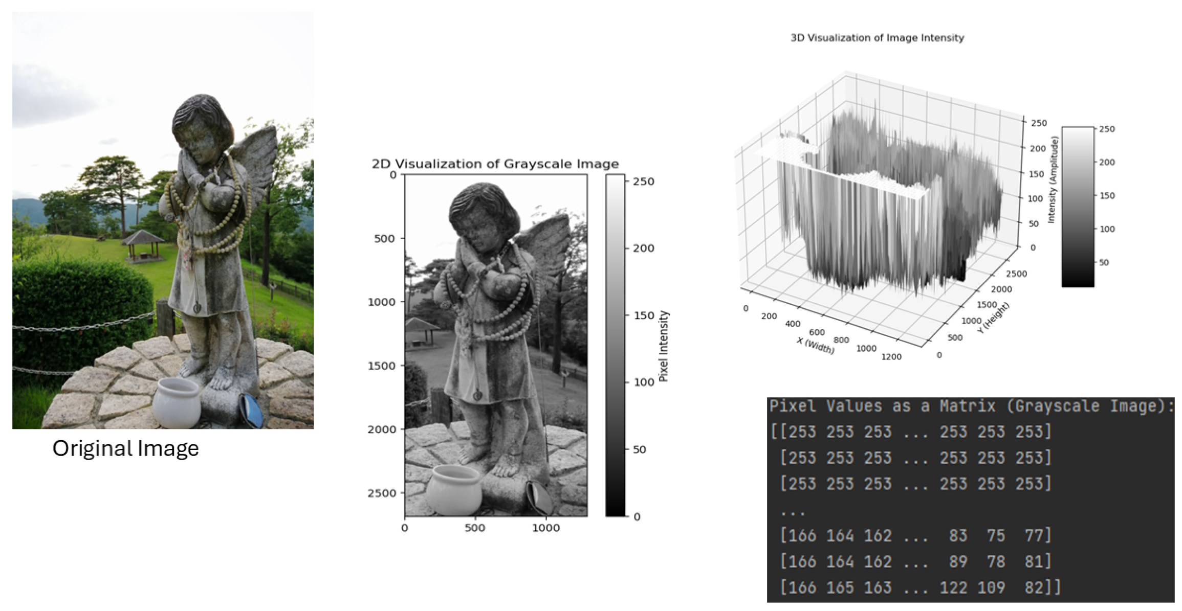
Figure 2.
Visualizing the edges of an digital images by Canny[16] edge detection.
Figure 2.
Visualizing the edges of an digital images by Canny[16] edge detection.
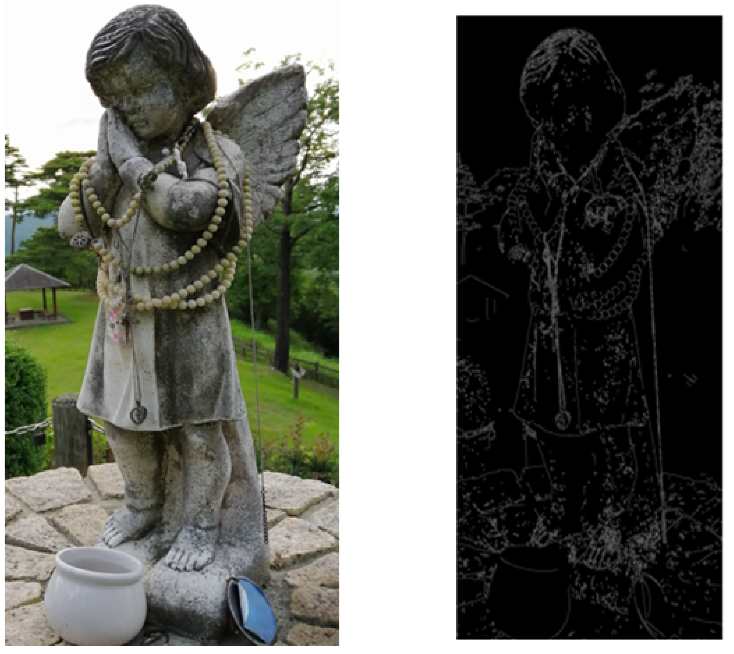
Figure 3.
Representing the HOG features. The original image and grayscale image are shown, and then the graph shows the orientation (degrees) and the gradient magnitude of all cells of the image. The second graph shows the histogram of the grayscale image where horizontal is pixel intensity and frequency is vertical.
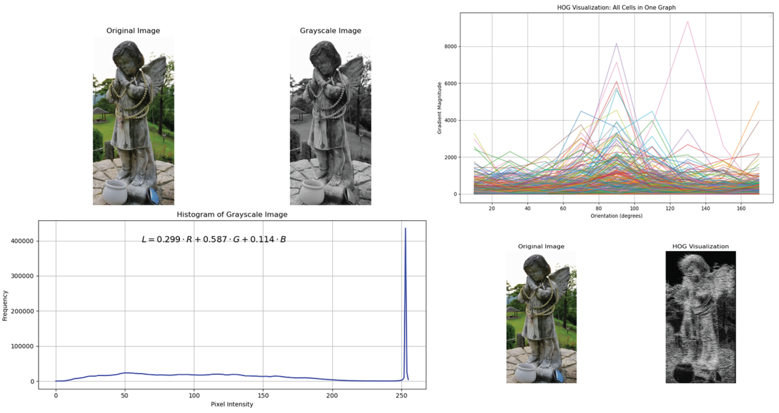
Figure 4.
An occlusion was created and detected. In this image, there is an original image, followed by an occluded image, and occlusion detection in that image.
Figure 4.
An occlusion was created and detected. In this image, there is an original image, followed by an occluded image, and occlusion detection in that image.
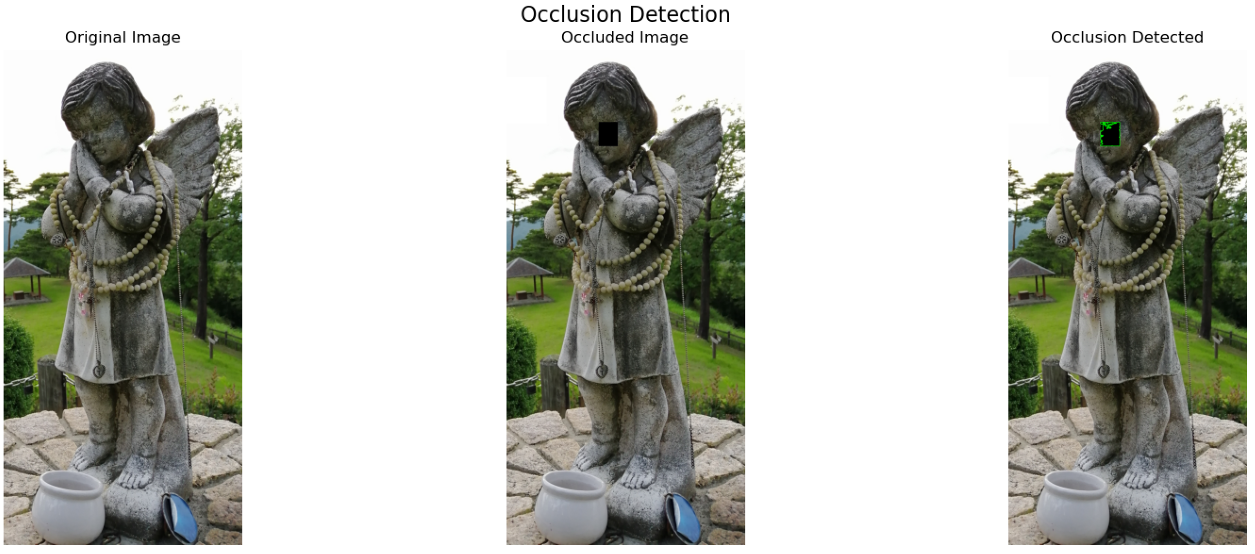
Figure 5.
Simple representation of a digital image.
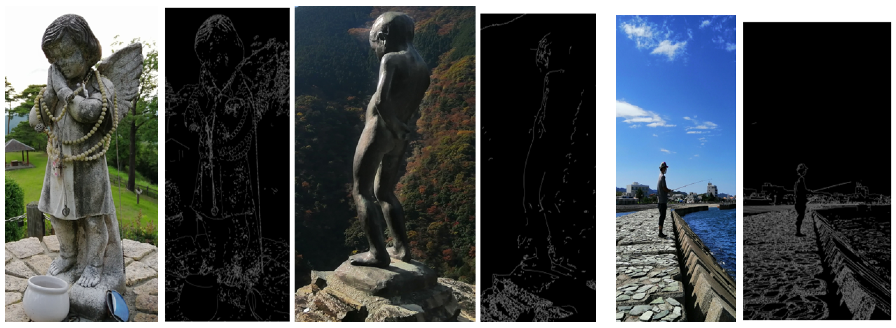

Table 1.
Comparison between Traditional Methods and Deep Learning-Based Method
| Aspect | Traditional Methods | Deep Learning-Based Methods |
|---|---|---|
| Feature Extraction | Handcrafted features such as SIFT (Scale-Invariant Feature Transform) and HOG (Histogram of Oriented Gradients), requiring manual selection and tuning of features based on domain knowledge. | Features are automatically learned from data through neural network architectures, such as CNNs (Convolutional Neural Networks), which extract relevant features directly from images without human intervention. |
| Performance | Traditional methods perform well in simpler tasks with smaller datasets, where problems can be clearly defined with rules or heuristics. They struggle with more complex tasks and require significant manual feature engineering. | Deep learning-based methods excel in handling more complex tasks, especially in large-scale environments or where data has high variation. These methods can tackle intricate patterns and dense environments with superior accuracy. |
| Robustness | Traditional methods are highly sensitive to noise, lighting variations, scale, and perspective. They rely on fixed features, which may not generalize well to different conditions. | Deep learning-based methods, such as CNNs, are more robust to noise, changes in scale, and perspective, as they learn to adapt from large datasets and generalize well to unseen data. Advanced architectures and data augmentation techniques improve robustness. |
| Data Requirements | Traditional methods typically require less data as they depend on handcrafted features, which can work with smaller datasets. These methods perform well in tasks with limited data. | Deep learning-based methods require large amounts of labeled data to effectively train models. A significant amount of data is needed to learn complex representations and relationships, especially for tasks like image classification and object detection. |
| Examples | Examples include edge detection (Canny, Sobel), feature matching (SIFT, ORB), and histogram-based methods (e.g., color histograms for object recognition). These are applied to simpler tasks like basic image processing and feature-based matching. | Examples include image classification (CNNs), object detection (YOLO, Faster R-CNN), and semantic segmentation (U-Net). These are used for more complex tasks like autonomous driving, facial recognition, and medical imaging. |
Disclaimer/Publisher’s Note: The statements, opinions and data contained in all publications are solely those of the individual author(s) and contributor(s) and not of MDPI and/or the editor(s). MDPI and/or the editor(s) disclaim responsibility for any injury to people or property resulting from any ideas, methods, instructions or products referred to in the content. |
© 2025 by the authors. Licensee MDPI, Basel, Switzerland. This article is an open access article distributed under the terms and conditions of the Creative Commons Attribution (CC BY) license (http://creativecommons.org/licenses/by/4.0/).
Copyright: This open access article is published under a Creative Commons CC BY 4.0 license, which permit the free download, distribution, and reuse, provided that the author and preprint are cited in any reuse.


