Submitted:
05 June 2025
Posted:
09 June 2025
Read the latest preprint version here
Abstract
Bell’s inequality is supposed to be universally valid. No local theory should violate it with space-like separated observables. Yet, classical mechanics is full of counter examples, especially in the case of binary energy redistribution. The explanation is that “space-like separation”, as used in Bell’s argument, is not a theory-independent concept. It only applies to models with jointly distributed variables, where coordination between measurements is required for Bell violations. In contrast, alternative transformations cannot influence each other in classical physics, yet they still display “non-classical” patterns of coincidence. This is demonstrated with a macroscopic fluid splitter that has the same output distributions and the same correlations as a Stern-Gerlach quantum spin analyzer.
Keywords:
quantum mechanics
; classical mechanics
; local realism
; bell's theorem
Introduction
“Locality” is shorthand for “no action at a distance” in modern physics. The question is how to express this concept formally, in terms of measurement outcomes? When two observables are well separated in space, they can still be statistically dependent for local reasons, by virtue of a prior common cause. This makes them conditionally separable, even if they are otherwise inseparable:
P(A,B) ≠ P(A) P(B)
P(A,B| λ) = P(A| λ) P(B| λ).
A known problem of this expression is distinguishability. Both types of correlation (with and without mutual dependence) entail the same range of coefficients. Therefore, it does not seem possible to confirm or to refute locality with direct observations. Yet, John Bell appeared to find a solution [1]. If three (or more) joint probabilities are considered together, then a distinguishable outcome is derived:
1 + P(B,C) ≥ |P(A,B) – P (A,C)|
This inequality is always obeyed when the three observables have simultaneous values, but it can be violated if individual terms are adjusted “by hand”. Thus, loophole-free Bell violations appear to require coordination at a distance. Nonetheless, this is not a necessary conclusion. The problem is that inequality (3) requires three separability conditions at the same time:
P(A,B| λ) = P(A| λ) P(B| λ).
P(A,C| λ) = P(A| λ) P(C| λ).
P(B,C| λ) = P(B| λ) P(C| λ).
Yet, any single event (such as A) is only considered in two combinations (with events B and C). Does the inequality (3) reflect the objective limits of conditional separability for A, or is it instead defined by the narrower criterion:
P(A,B,C| λ) = P(A| λ) P(B| λ) P(C| λ).
As we know today, Bell’s inequality applies exclusively to systems with jointly distributed variables [2,3,4]. Therefore, it is inconclusive about locality in the most general sense.
A possible way out is to express the conditional independence of an observable A without irrelevant relationships, such as P(B,C). Indeed, this is a well-known approach that leads to the so-called “no-signaling” criterion:
P(A| a, b) = P(A| a, c)
The average probability of event A is the same no matter which other observable is chosen for joint measurement. As shown by Popescu and Rohrlich [5], this criterion allows for maximal (“super-quantum”) Bell violations. Hence, a more general definition of event independence leads back to the problem of distinguishability: we cannot use experimental evidence to falsify locality. Surprisingly, the standard interpretation of expression (8) is that it includes the effect of “non-signaling non-locality”. Without being anchored in a precise definition of λ, it cannot be proven to contain consistent pairings for each iteration. On the one hand, this argument is inconclusive. On the other hand, it seems wise to avoid controversy and to attempt a different strategy. Is it possible to formalize the essence of locality without average probabilities?
Consider two observers, Alice and Bob. Locality entails that individual measurement outcomes for Alice are the same no matter what Bob is doing. Therefore, two joint distributions (C,A) and (A,B) must always agree about the values of A. Similarly, (B,C) and (C,A) must always agree about the values of C, and so on. This feature is known in probability theory as “pairwise consistency”. Moreover, Bell experiments require closed chains of double measurements that are also known as Vorob’ev cycles [6,7]. Such arrangements can be consistent without joint distributions. Even maximal Bell violations are possible with fixed individual outcomes [8]. Hence, “non-signaling behavior” and local behavior are equally immune to Bell’s Theorem. Indeed, numerous recent studies have converged on the same conclusion: Bell’s inequality is just a consequence of statistical compatibility [8,9,10,11,12,13,14,15]. Unfortunately, every known attempt to explain quantum entanglement with “Local Realism” has failed [16,17]. How can it be that something is theoretically commonplace and practically inaccessible at the same time? This is an interpretive problem. If non-commuting variables are attributed to mutually exclusive measurements, then Bell violations require loopholes (or new physics). If they are assigned to objectively incompatible properties instead, then quantum correlations are fundamentally classical.
Measurements vs Transformations
Classical wave interactions are often analyzed with vector decomposition. For example, a laser beam with diagonal polarization can be split into two components (vertical and horizontal) with a polarizing beam-splitter (PBS). The magnitude of the input amplitude is equal to the vector sum of the two output amplitudes (Figure 1). Yet, the ontological implications of this process are ambiguous. On the one hand, we could assume that macroscopic phenomena reflect microscopic processes. If the input projection is diagonally polarized, then all the photons in it are also diagonally polarized. This leads to the “transformation hypothesis” about vector decomposition: the PBS induces predictable physical changes, while conserving angular momentum. In this case, diagonally polarized input photons are rotated into the vertical or horizontal output planes. On the other hand, we could also treat the macroscopic net state as an optical illusion. The “deeper reality” could be that half the photons are vertically polarized, while the other half are horizontally polarized from the source. This leads to the “measurement hypothesis” in which the PBS works as an inert filter. The beam-splitter is assumed to reveal the hidden input state of the photons without perturbation, just as captured by vector decomposition. Of course, pre-modern classical physics invoked component “modes of oscillation”, rather than light quanta, but the basic intuition is the same. For this discussion, the important detail is that the measurement hypothesis was perceived as unquestionable by the end of the 19th century.
As we know today, individual quanta do not express the values of isolated components prior to measurement [18]. Yet, looking back at the history of modern physics, we see that the classical “measurement hypothesis” was never discarded. Instead, it was taken over by the Copenhagen interpretation and converted into the “quantum measurement problem”. In this approach, diagonally polarized laser beams were still presumed to contain two “modes of oscillation” from the source (vertical and horizontal). Yet, individual quanta were presumed to express both of them at the same time, until they were “collapsed” by the act of measurement. According to Niels Bohr, this view was forced by the failure to “classical realism” to capture unobservable quantum dynamics. His favored solution was to restrict intuitive explanations to the domain of measurement outcomes [19]. The well-known problem of this approach, as pointed out by Einstein, Podolsky and Rosen (EPR) [20], is that many quantum properties can be predicted without observation, especially in the case of entangled systems. A better solution was surely possible. Unfortunately, the chosen alternative was to return yet again to the classical version of the “measurement hypothesis”. According to modern “Local Realism”, individual quanta from a diagonally polarized laser beam (Figure 1) cannot be objectively diagonal. Instead, they must be objectively polarized in either the vertical or the horizontal plane, in case they are measured in the vertical basis. Yet, many other measurement bases are equally available. Therefore, individual photons are presumed to have multiple sharp states of polarization at the same time. After all, non-commuting variables (just like quantum momentum and position) are expected to be simultaneously real in this approach. Not only is this interpretation non-physical, but it also leads to bad predictions. If mutually exclusive properties have well-defined “real” values at the same time, then non-commuting quantum operators correspond to jointly distributed classical variables. As shown by Bell’s Theorem, this leads to verifiable contradictions with quantum theory. Given the results of recent loophole-free experiments [21,22,23,24], it follows that “Local Realism” is both ontologically and empirically problematic. By implication, the “measurement hypothesis” is a dead end. Meanwhile, the “transformation hypothesis” remains unexplored.
Consider a billiard ball, moving on a flat surface towards another physically identical ball (Figure 2A). Numerous patterns of collision are possible, with kinetic energy being split 50-50, 0-100, or any other fraction. This does not show that a billiard ball is moving in every possible direction at the same time. Vector decomposition only shows what can happen in various alternative collision scenarios, with binary patterns of energy redistribution. (Output components for different bases of transformation are mutually exclusive. Contradictions emerge if they are treated as real at the same time). If a ball is in motion, relative to the table surface, it has a well-defined state of momentum (p=mv) and a corresponding amount of kinetic energy (Ek=mv2/2). In the event of an elastic collision, a fraction of momentum is transferred to the second ball. This can be predicted with vector decomposition, by taking into the account the cosine of the angle between the input and output velocity vectors. However, kinetic energy is proportional to the squared scalar magnitude of the velocity vector. This is the same “Malus Law” that we see in the interaction between a classical laser beam and a PBS [25]:
where “I” corresponds to irradiance for optical projections, subscripts “T”, “R”, and “in” differentiate between “transmitted”, “reflected” and “input” projections respectively, while “θ” is the angle between input and transmitted planes of optical polarization. Accordingly, an ideal diagonal collision between these balls entails a 50-50 pattern of energy redistribution (Figure 2A). The key feature of this rule is that binary energy redistribution is not linear. Mutually exclusive patterns (governed by the cosine squared rule) are physically and numerically incompatible. For example, the two billiard balls can also collide at 22.5 degrees. This means that 85% of the input energy will be transferred from the first ball to the second (cos222.5), rather than 75% corresponding to the midpoint between 100% and 50%. Moreover, the second ball can also experience a 22.5˚ collision with a third ball, resulting in a final output direction of 45˚, relative to the direction of motion of the first ball (Figure 2B). This means that two collisions with a total deflection of 45˚ can transfer 72% of input energy, even though a single collision at 45˚can only transfer 50%. Alternative patterns of energy redistribution cannot be reconciled with each other. Therefore, such variables cannot be jointly distributed. More importantly, they cannot correspond to “hidden” vector components that are somehow simultaneously real, as suggested by the modern concept of Local Realism.
IT = Iin cos2θ
IR = Iin sin2θ
Bell violations with alternative transformations
Classical particles and classical waves display the same non-linear patterns of energy redistribution. However, these transformations are governed by system-level interactions, with an interesting caveat. In the case of billiard ball collisions, a single ball represents a full macroscopic system. It is able to transfer kinetic energy according to non-linear rules, but we cannot meaningfully “quantize” the motion of a billiard ball into detectable increments. In contrast, optical projections have a natural correspondence between macroscopic energy redistribution and microscopic single-event distributions. After all, wave energy is proportional to the amplitude squared, which is also proportional to the number of quanta in the same projection:
Ew = kA2 = nFh.
At the quantum level, we use system-level predictions, captured by wave-functions, to predict the probability of detecting single events, also by squaring relevant amplitudes with Born’s rule:
P(ai) = |<ai|ψ>|2.
Hence, there is a natural way to convert system-level energy redistribution into expectation values for various patterns of coincidence at the individual level. For a CHSH experiment, the task is simply to identify a rotationally invariant pattern of energy redistribution, which can be achieved with depolarized optical projections. Yet, this phenomenon is already associated with non-physical interpretations that hinder the analysis of quantum correlations. Is it possible to find a classical system that can better elucidate the local nature of Bell violations?
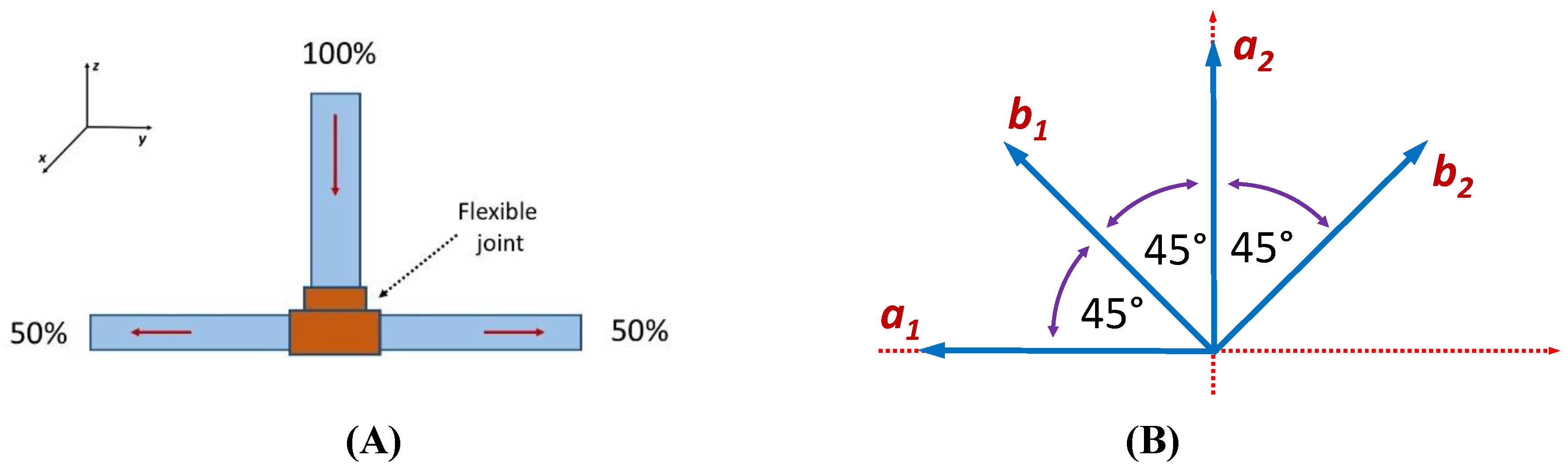
Consider a flexible fluid-splitter, as shown in Figure 3A. The vertical pipe feeds some kind of fluid into a flexible T-junction with two output pipes leading in opposite directions. The input pipe is rigid in the z-direction, while the output axis can be rotated at will in the x-y plane. Fluid is pumped into this system under pressure and is split 50-50. For example, half of the fluid could be directed into the “plus” y-direction and the other half into the “minus” y-direction. Though, imagine that we freeze the process, and ask a counterfactual question. How much fluid from the “plus” output would have been in the same pipe, if the axis of the splitter was rotated in the x-y plane by an arbitrary angle? To answer this question, we need to assume that fluid splitting is a fundamentally deterministic process. It is not an accident that the molecules from the “plus” output are found in this channel. Ergo, if the same exact process were to be replayed again, the same exact molecules of fluid would be found in the same output. That being said, we are not dealing with independent ballistic particle trajectories. The motion of fluid molecules is inseparable from the motion of the fluid as a whole. The question is: how does the fluid, as a macroscopic system, interact with the walls of the flexible fluid splitter?
A plausible assumption in this scenario is that a reference output direction “a+” is associated with a conserved amount of kinetic energy carried by the fluid. Furthermore, transverse redistribution of kinetic energy into some new orientation “b+” is known to follow a cosine squared law:
Ekb+ = Eka+ cos2(θ/2) + Eka- sin2(θ/2).
If a given sliver of fluid has a fixed amount of kinetic energy in the a+ direction, then it can only impart a fraction in the b+ direction, determined by the cosine squared of half the angle between the two orientations. The other amount of kinetic energy, to maintain rotational invariance, must come from the opposite (a-) direction. Yet, notice that the magnitude of fluid velocity does not change under transverse redirection in the fluid splitter. The fluid pressure inside the pipes remains constant. Therefore, the cosine squared law must be physically satisfied by a non-linear redistribution of fluid mass between alternative directions. The mass of the fluid in any new direction b+ must be composed of cosine-squared of half the angle from the mass that was emitted in the a+ direction, plus a supplementary amount from the a- direction:
Mb+ = Ma+cos2(θ/2) + Ma-sin2(θ/2).
Assuming uniform fluid density, it follows that the probability of any fluid molecule to display correlated behavior between two alternative orientations is also non-linear:
P(B+|A-) = P(A-) cos2(θ/2).
In other words, the proportion of fluid molecules that can also emerge in the “plus” channel for direction b given that they emerged in the “plus” channel for direction a, is determined by the cosine squared of half the angle between the two directions. This translates into corresponding probabilities at the level of single molecules. For example, if the output axis was shifted by 45˚ relative to the y-axis, then 85% of the water molecules would have been the same in the “plus” channel, while 15% would have traded places with the “minus” channel. On the one hand, we have a system-level effect that is observable as fluid motion. On the other hand, we have molecular behavior expressing the non-linear features of this macroscopic process.
The offshoot of this description is that we have rotationally invariant correlations between any two output settings for the fluid-splitter. It does not matter which axis is chosen for reference and which transformation is added for correlation analysis. One way or another, 50% of the input fluid would end up in the “plus” channel. For any other output orientation, the proportion of the molecules that would have been in the same channel (and the supplementary proportion that trade places) are determined by the cosine squared of half the angle between the two settings. This means that we can choose several adjacent orientations, separated by 45˚ angles, as shown in Figure 3B. To keep the analogy with a CHSH quantum experiment [26], we can label these directions as a1, b1, a2 and b2. Just as described above, we can ask: what proportion of molecules would have been correlated for any of the possible pairwise combinations? The answer is that three combinations are separated by 45˚, with a final coefficient of correlation of:
In contrast, the last combination spans an angle of 135˚. Therefore,
We can plug these four expectation values into the CHSH expression for a Bell test with four variables [26]:
SCHSH = |E(A1,B1) – E(A1,B2) + E(A2, B1) + E(A2, B2)| ≤ 2
As a result, we obtained a Tsirelson violation of the CHSH inequality [27], just as predicted for quantum correlations between two entangled electron beams. However, we derived this behavior for alternative orientations of a single classical fluid splitter. This was done deliberately, to clarify the local nature of these correlations. All the settings of a Bell experiment with photon polarization or electron spin correspond to various incompatible transformations that can happen in one and the same system, locally. They just happen to obey nonlinear rules.
Of course, it is not possible to observe the same exact molecules in two different scenarios in one step. This was an exercise in counterfactual analysis, as if we had the ability to replay the same physical process in different alternative ways. However, it is possible to simulate the behavior of a fluid with molecular level precision in a modern computer. Furthermore, it is possible for two different computers to play back the same simulation from the source to the flexible neck of the fluid splitter. In this case, one computer named Alice can choose between two output settings (such as 0˚or 90˚, relative to the y-axis), while another computer named Bob can choose between two other settings (such 45˚ and 135˚, relative to the y-axis). The settings for both Alice and Bob can be chosen at random, or supplied by a third party, or even pre-arranged in advance. It does not matter how the settings are chosen, since – in the end – only four combinations are possible, as explained above. (This is an important conclusion, given that “freedom of choice” is an essential requirement for loophole-free Bell experiments). The correlations between these settings are rotationally invariant and obey the cosine squared law. Yet, this law does not describe non-local effects between the measurements of Alice and Bob. As shown above, these are natural types of behavior that can happen locally in each system, during binary energy redistribution. Similarly, Alice and Bob could be making coincidence studies with identically stacked decks of playing cards. In both cases, the correlations would be local. The difference is that the properties of playing cards are jointly distributed and cannot violate Bell-type inequalities.
This thought experiment can even be extended to “single event” detection schemes. For example, it is possible to inject die molecules into the fluid, one at a time, and to observe their fate at the output: do they emerge in the “plus” or “minus” output pipe for any chosen setting? The behavior of die molecules would also be inseparable from the behavior of the fluid as a whole. Therefore, their output statistics, and the corresponding correlations between Alice-Bob simulations, are expected to display the same patterns as described above. Upon closer inspection, this is not very different from quantum behavior, where individual-level statistics are governed by system-level (quasi-macroscopic) effects, as captured formally by quantum wave-functions. By implication, quantum behavior is also local.
Conclusion
As a corollary of the above, we have a straightforward demonstration of quantum-like behavior in a classical system. Individual molecules as part of a macroscopic fluid can display rotationally invariant 50-50 distributions, and rotationally invariant correlations between alternative settings, just as seen in Stern-Gerlach devices that study electron spin. Surprisingly, this type of behavior is common in classical systems, especially in the case of mutually exclusive transformations with binary energy redistribution. This is definitive proof that Bell violations can emerge from local correlations for incompatible variables, as predicted by numerous studies in the past [7,8,9,10,11,12,13,14,15]. As it turns out, the gap between classical and quantum phenomena is not ontological. “Classical” (pre-modern) theories produced incorrect microscopic predictions, yet this was due to unfortunate interpretive choices for ambiguous quantitative relationships. It is not the principles of “Classical Realism” that are to blame, but rather the downstream effects of several contingent assumptions. Therefore, this is not a problem that can be solved with mathematical or experimental proof alone. Interpretive problems require interpretive solutions. In this case, the hard part was to identify the classical “measurement hypothesis” as ontologically misleading, and to acknowledge the fundamental role of transformations in binary energy redistribution. In retrospect, the Copenhagen interpretation identified the problem correctly, but chose to reject classical mechanics, instead of correcting it. This launched a long debate between two non-physical solutions, while the “transformation hypothesis” was waiting to be rediscovered.
References
- Bell JS. Speakable and Unspeakable in Quantum Mechanics (Cambridge, 1987).
- Fine A. Joint distributions, quantum correlations, and commuting observables, J. Math. Phys. 1982, 23: 1306. [CrossRef]
- De Muynck WM, De Baere W, Martens H. Interpretations of quantum mechanics, joint measurement of incompatible observables, and counterfactual definiteness, Found. Phys. 1994, 24: 1589. [CrossRef]
- Son W, Andersson E, Barnett SM, Kim MS. Joint measurements and Bell inequalities, Phys. Rev. A 2005, 72: 052116. [CrossRef]
- Popescu S, Rohrlich D. Quantum Nonlocality as an Axiom. Found. Phys. 1994, 24: 379.
- Vorob’ev NN. Consistent Families of Measures and Their Extensions, Teor. Veroyatnost. i Primenen. 1962, 7:153. [CrossRef]
- Hess K, Philipp W. Bell’s theorem: Critique of proofs with and without inequalities, AIP Conf. Proc. 2005, 750: 150.
- Hess K, Philipp W. A possible loophole in the theorem of Bell. Proc Natl Acad Sci USA 2001, 98:14224. [CrossRef]
- Khrennikov A. Bell-Boole Inequality: Nonlocality or Probabilistic Incompatibility of Random Variables? Entropy 2008, 10: 19. [CrossRef]
- Nieuwenhuizen TM. Is the contextuality loophole fatal for the derivation of Bell Inequalities? Found. Phys. 2011, 41: 580. [CrossRef]
- Jung K. Violation of Bell's inequality: Must the Einstein locality really be abandoned? J. Phys.: Conf. Ser. 2017, 880: 012065.
- Khrennikov A. Get Rid of Nonlocality from Quantum Physics, Entropy 2019, 21: 806. [CrossRef]
- Cetto AM, Valdés-Hernández A, de la Peña, L. On the Spin Projection Operator and the Probabilistic Meaning of the Bipartite Correlation Function, Found. Phys. 2020, 50: 27. [CrossRef]
- Cetto AM. Electron Spin Correlations: Probabilistic Description and Geometric Representation, Entropy 2022, 24: 1439. [CrossRef]
- Hess KA. Critical Review of Works Pertinent to the Einstein-Bohr Debate and Bell’s Theorem, Symmetry 2022, 14: 163. [CrossRef]
- Larsson JÅ, Loopholes in Bell inequality tests of local realism, J. Phys. A 2014, 47: 424003. [CrossRef]
- Larsson JÅ, Gill RD. Bell's inequality and the coincidence-time loophole, Europhys. Let. 2004, 67: 707. [CrossRef]
- Peres A. Quantum Theory: Concepts and Methods (Kluwer, 1993). [CrossRef]
- Plotnitsky A. Niels Bohr and Complementarity: An Introduction (Springer, 2012).
- Einstein A, Podolsky B, Rosen N. Can Quantum-Mechanical Description of Physical Reality Be Considered Complete? Phys. Rev. 1935, 47: 777. [CrossRef]
- Hensen B, et al. Loophole-free Bell inequality violation using electron spins separated by 1.3 kilometres, Nature 2015, 526: 682. [CrossRef]
- Giustina M, et al. Significant-loophole-free test of Bell's theorem with entangled photons, Phys. Rev. Lett. 2015, 115: 250401.
- Shalm LK, et al. A strong loophole-free test of local realism, Phys. Rev. Lett. 2015, 115: 250402. [CrossRef]
- Rosenfeld W, et al. Event-Ready Bell Test Using Entangled Atoms Simultaneously Closing Detection and Locality Loopholes, Phys. Rev. Lett. 2017, 119: 010402. [CrossRef]
- Hecht E. Optics (Addison-Wesley, 2001).
- Clauser JF, Horne MA, Shimony A, Holt RA. Proposed Experiment to Test Local Hidden-Variable Theories, Phys. Rev. Lett. 1969, 23: 880. [CrossRef]
- Cirel’son BS. Quantum generalization of Bell’s inequality, Lett. Math. Phys. 1980, 4: 93.
Figure 1.
Classical vector decomposition with ambiguous implications. A linearly polarized laser beam is split 50-50 by a polarizing beam-splitter (PBS). The outcome is predicted with vector decomposition, as shown. Does it follow that the beam is made of two “real” components that are measured by the PBS, or is this simply the outcome of a physical transformation? The first option is at the root of numerous problems in modern physics.
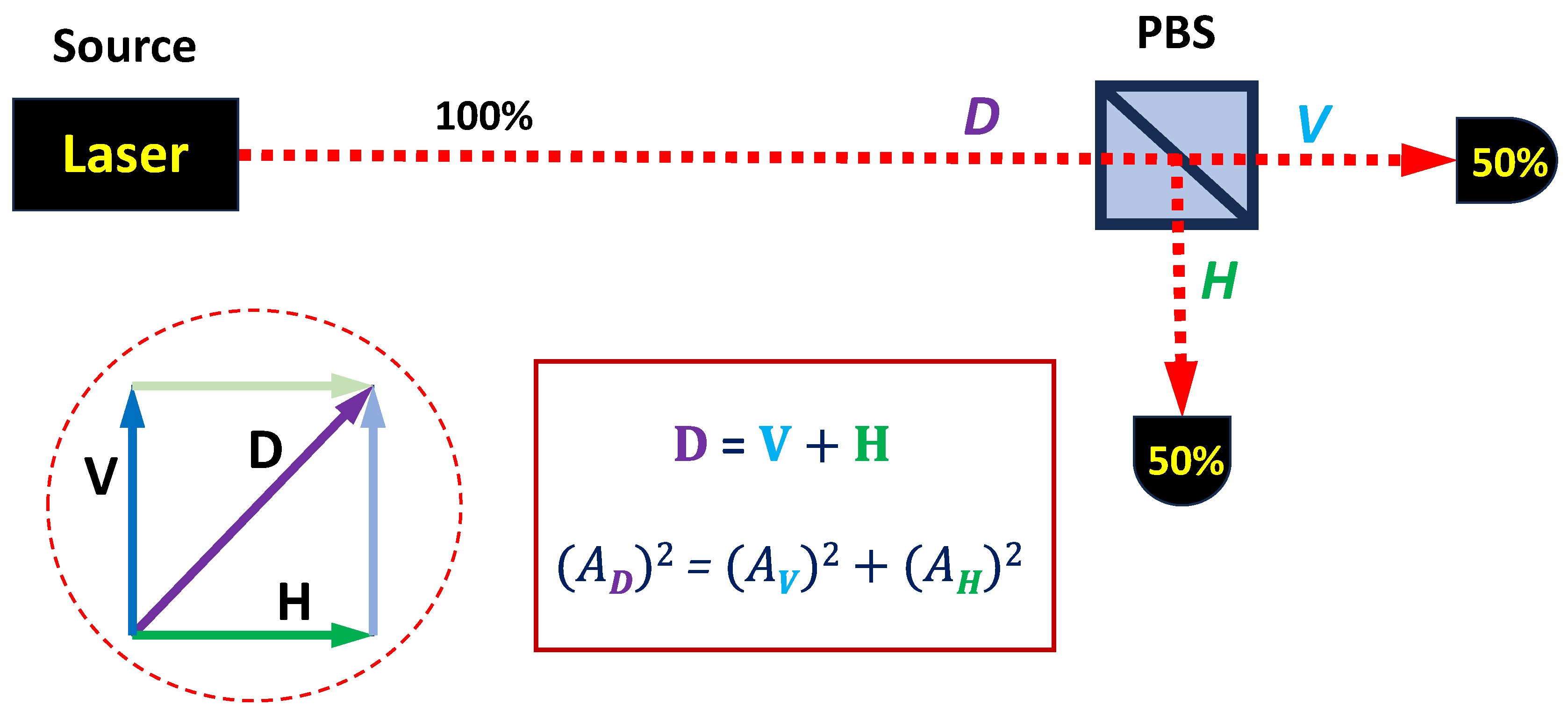
Figure 2.
Energy redistribution with incompatible outcomes. Classical velocity vectors can be decomposed into virtual pairs of components that correspond to the expected new value in any direction, in the event of a lossless elastic collision. The amounts of corresponding “available momentum” in each direction are proportional to the cosine of each angle of deflection. Yet, the redistributed amounts of kinetic energy are proportional to the cosine squared of the same angles. (A) An elastic collision at 45° between two billiard balls on a slate table results in a transfer of 50% of the input amount of energy. (B) The same final direction of motion can be achieved with two sequential collisions at 22.5° each. Yet, the final amount of energy in this case is 72%. It is not possible to reconcile the effect of two operations of redistribution at 22.5° with a single operation at 45°. This fundamental incompatibility between alternative outcomes is the source of Bell violations, both at the classical and at the quantum level.
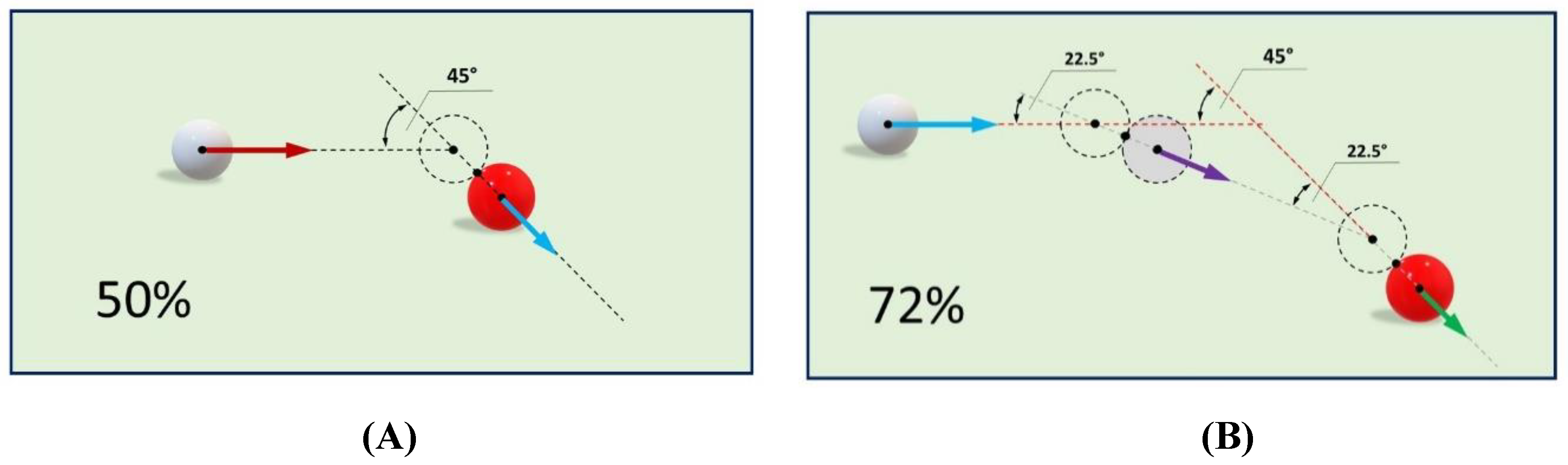
Figure 3.
Classical analogue for Stern-Gerlach electron behavior. CHSH experiments require alternative incompatible properties and rotational invariance for Bell violations. These conditions are satisfied by energy redistribution patterns in fluid flow-splitters. (A) Basic diagram of the mechanism. Fluid flows downward in the input pipe and is redistributed 50-50 between the two output pipes. The horizontal section is flexible, relative to the vertical channel. It can be rotated at will in the x-y plane. For any two directions, some fluid molecules will emerge through the same output pipe, and others will trade places. The proportion of identical outcomes is proportional to the cosine squared of half the angle between two randomly selected directions. This can be used to make a Bell experiment, by simulating two identical systems with microscopic precision in adequate computers. (B) Visual aid for understanding the possible combinations in a CHSH experiment. Alice can switch at random between two orthogonal orientations (a1 or a2), while Bob alternates between the other two (b1 or b2). Only four combinations are possible, such that three of them are separated by 45° and one by 135°. The end result is a quantum-like Bell violation.
Disclaimer/Publisher’s Note: The statements, opinions and data contained in all publications are solely those of the individual author(s) and contributor(s) and not of MDPI and/or the editor(s). MDPI and/or the editor(s) disclaim responsibility for any injury to people or property resulting from any ideas, methods, instructions or products referred to in the content. |
© 2025 by the authors. Licensee MDPI, Basel, Switzerland. This article is an open access article distributed under the terms and conditions of the Creative Commons Attribution (CC BY) license (http://creativecommons.org/licenses/by/4.0/).
Copyright: This open access article is published under a Creative Commons CC BY 4.0 license, which permit the free download, distribution, and reuse, provided that the author and preprint are cited in any reuse.


