Submitted:
30 May 2025
Posted:
05 June 2025
Read the latest preprint version here
Abstract
Image segmentation in light field imaging is a fundamental problem in digital image processing and analysis, with broad applications in areas such as augmented reality, healthcare, and biomedical imaging. While numerous algorithms have been proposed primarily leveraging convolutional neural networks and deep learning approaches to estimate depth and define pixel clusters this work introduces a novel pipeline that integrates light field depth estimation with the directed random walk algorithm, a method frequently used for refining depth maps. We evaluated our approach using both a controlled 4D Light Field Benchmark dataset and a real-world image database. Although the algorithm showed difficulty improving depth quality in real-world conditions due to increased noise and uncontrolled environments it maintained computational efficiency and demonstrated promising results when compared to existing techniques. These outcomes suggest that our method offers a viable alternative to heavier deep learning models and opens new avenues for future research in light field-based image segmentation.
Keywords:
depth estimation
; light fields
; image segmentation
; depth map algorithms
; 3D reconstruction
; multi-view imaging
; image analysis
; depth perception
; algorithm evaluation
I. Introduction
Depth estimation for different types of data remains a challenge in digital image analysis for scenarios such as indoor spaces, where a detailed 3D model is of particular importance for robotic and autonomous navigation. However, with the advent of virtual and mixed reality devices, this problem became of even greater interest, now having to deal not only with indoor data but also with scenes with great variation of depth and even with noise added by the devices during the acquisition of the footage [1]. This study presents a complete pipeline with all the stages of multiple depth map estimation, from RGB image generation to random combination of these algorithms' trained networks to generate a much smaller set of models, which will be used as a single-stage architecture for depth map estimation using light fields. We will first use multiple object detectors to generate different scenes in the training set that are realistic diving pool balls augmented to be training samples for the network we train with light field images. In terms of this work, we show that it is possible to learn good depth estimates from data generated by depth estimation by other models.
We present a brief review of the state-of-the-art methods for depth estimation, highlight their main differences, and show how well each one behaves in both indoor and outdoor scenarios. In order to follow this research, it is assumed that the reader has a full understanding of image analysis, and the calculations involved, regardless of the algorithm used, or has access to the respective mathematical representation. In the end, we show that, despite the incredible 4D Light Fields Benchmarks training data that light fields present for depth estimation, one should always be careful not to arrive at unrealistic results due to texture losses. We display results that arise in situations with deep focus variation or occlusion areas in the point clouds.
II. Motivation and Objective
In recent work, the use of light fields for the task of depth estimation has attracted a considerable amount of interest. Given different advantages over monocular stereo techniques, LF-based depth estimation has proven useful for challenging visual computing tasks. These advantages include the ability to generate detailed depth maps from the complexity of the data, avoidance of disparity search, disparity estimation, and occlusion handling in occluded object areas, and handling of object distortion in novel views. In the context of light field imaging, having an appropriate depth map has been known to be an important factor for synthesizing accurate novel viewpoints. In term of both rendering a novel view and generating an accurate depth map, content creators can provide a higher-quality experience to viewers, leading to better immersion with less distortion.
However, quality challenges add to the fact that the light fields have inherently low resolution when represented with optical elements and diffusion. Many light fields are designed with similar properties in mind, but other light field variants may lack such dense plenoptic sampling, leaving gaps that lead to inaccurate depth maps. In addition to containing several inconsistencies and predicting errors in the occluded regions, deep learning frameworks are incompatible with the occlusions of the light fields. This study presents several advances in the state of the art of the literature on light field depth estimation, enabling us to provide a channel for the implementation and investigations of such initiatives and accelerating the lattice-based means of the dense light field depth estimation algorithms by learning the multi-monomer occlusions [2].
We discuss how to train for much larger variations of datasets that still approach the plenoptic function, report on solutions to learn beyond practical resolution limits of real light fields, present a deep learning-based multi-plane light field depth estimation algorithm, and provide an extensive comparison of state-of-the-art algorithms in the direction of error and occlusion. In terms of these investigations, we tailor several state-of-the-art light field depth estimation benchmarks and report state-of-the-art error measures on these calibrated datasets with a benchmark suite dataset.
III. Related Works
Developing an accurate depth estimation algorithm that works on light fields while simultaneously permitting real-time operation remains an open problem. The recent popularity of deep learning algorithms in depth estimation has shown significant improvements, both in supervised and unsupervised depth estimation. Light field-based depth estimation should also gain an advantage by incorporating a depth prior based on far fewer training images than required in other depth estimation approaches since light fields can provide unique 4D spectral spatial information. The performance was also further improved by optimizing the latent dimension for angular accuracies, which is the natural domain for the light field utilized for segmentation applications. However, depth estimation algorithms might still not be competitive compared to conventional methods if the input scene is not from a specialized domain or if a strong estimating model is not available [3].
Considering the applications of light field technologies, refocus, and synthetic aperture processing for several imaging concepts, this could be extremely useful for various applications that tradeoff between depth of field, spatial resolution, and viewing angle constraints. Tackling computational complexity, many recent works utilize either simplified dimensions in the training pipeline or inference with processing tailored to each target application. The former suggests certain robustness in the descriptor-based model, but the robustness seems to degrade when the discriminator is shallow for inference from a fixed latent code.
IV. Methods
In this contribution, we discuss the use of a light field representation from a set of cameras and state-of-the-art disparity/depth estimation methods operating on this representation, namely, CNNs trained on light field image pairs [4]. While we focus on the task of estimating pixel-wise disparities and depth from a light field using these algorithms, we experimentally verify their applicability for the task of segmentation. Image segmentation is a computer vision task targeting the division of a given image into different regions. These regions are composed of pixels that have common characteristics such as color, intensity, and texture. The main objective of image segmentation is to break down an image into distinct, manageable regions, enhancing its clarity and making it more suitable for deeper analysis and interpretation.
Image segmentation aims to group together those pixels that have some associated meaning but are different from others based on the values of the pixels' attributes, such as gray levels, color brightness, intensity, texture, and motion. Our work can be interpreted in the context of combining modules in a deep learning image analysis pipeline. Today, any state-of-the-art image analysis pipeline consists of two main modules: (1) a perceptual front-end to extract useful information from images, and (2) higher-level indexes to recover scene properties. Our source of input, a light field, provides multiple views of the scene, from which it is possible to create a depth map. This property is particularly attractive, as depth data can be very useful throughout various stages of the digital image processing, such as for inaccurate background prediction, which might wrongly associate a few pixels in the ground plane as part of a detected window classified as a person [5].
This is particularly important when performing automatic operations on the scene, such as object detection, object recognition, and scene analysis, especially when the image has a crowded body of people walking on the ground in the scene. We analyze the trade-offs of using trainable algorithms to predict disparity from the light field versus using classical refocusing as the basis for the application of these algorithms in the higher-level indices. Additionally, we show quantitative results proving the advantages of disparity estimation algorithms over traditional refocusing for use in higher-level indices.
Dataset
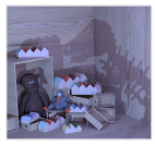
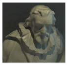
We are using the 4D Light Field Benchmark Dataset to the experiments is the development of a dataset that can be used for training the depth estimation method and the background estimation method. We make modifications to a well-known light field dataset to make it suitable for image segmentation applications. The dataset has only a small number of training and test images, but the images are high quality and contain challenging occlusion and foreground-background geometry. In order to provide ground truth depth images, we use the segmentation information available with the original dataset, which is constructed by human operators. Only the global segmentation information is used; at each pixel, labels available with the dataset indicate whether the pixel is known and belongs to the foreground or the background. These labels can be directly assigned to the known pixels in an image, while the unknown pixels are filled in by open-inpainting methods. The 4D Light Field Benchmark consists of a grid of 9 × 9 angular views, with each view captured at a spatial resolution of 512 × 512 pixels. We evaluated quantity based on three data points the Pascal VOC and Filter dataset light field object detection and segmentation with 17×17 views and 960 × 1280 resolution [6].
A. Least Squares Gradient (LSG) Method
Now, we present a brief summary of LSG solutions in the case of the RoI problem when using the disparity degree image. Consider the correspondence energy function, which is minimized over the pulse interval in a various particular way. Namely, different smoothness and data terms are applied. If the energy function does not contain discontinuity-preserving terms, the straightforward application of the RoI method results in the double local integrals, which gives several pixels satisfying. Thus, the output is interconnected subpixel accurate [7]. Such a RoI method that is independent of the determination of the neighboring pixels of the problem pixel does not belong to the app-fragment class of sound pixels interpolation methods. When a point of view is shifted, an image patch is also displaced as and . However, the lead's equation is the following equality:
L(x, y, u, v) = L(x − d∆x, y − d∆y, u + ∆x, v + ∆y)
We can use one additional term to obtain the app-square method, which is one among those having a much wider application area for light field sensors, including also non-planar ones. It does not modify the delta sensitivity at turning points and preserves the delta magnitude sensitivity at them. We modified the parameters of the L interpolation method; another derivative sensitivity in the simple turning points can also be preserved. Some other 3D sensor models based on RoI or Culmann integration methods were in the state of patent applications or patents describing the device construction. This connection has been restructured and reinterpreted for all picture patches as a squared error E, which will be reduced in proportion to d.
Consequently, by resolving the above optimization issue, we get the following conclusion:
The displacement between the object's image across all light field images is denoted by . In the context of light field analysis, spatial intensity variations are denoted x by and for the horizontal and vertical axes, respectively, whereas and correspond to gradients along the angular dimensions, capturing directional changes across different viewpoints.
B. Plane Sweeping Method
We applied another commonly used cost-volume creation method, the plane-sweeping algorithm. This leads to dense depth estimation given the set of multi-view images. The algorithm is designed to identify correspondences between the images, improve on epipolar scan-line correspondence techniques, and use the strength of cues such as inter-image color gradients and inter-image gradient pair changing trends. Based on the significant depth inconsistency regions of subsequent frames starting with a small number of frames, we present the concept of local planes to identify the relevant corresponding features [8]. Additionally, the performance will be enhanced with many points corrected. The light-field data undergoes 4D shearing to refocus each view to the center view, as demonstrated in the formula.
Let represent the disparity-adjusted light field view and L the original light field. The light field is parameterized using spatial coordinates ( x , y ) and angular coordinates ( u , v ), which are used to achieve horizontal and vertical alignment of the views. Following this alignment process, the images are stacked together, and a cost volume C is constructed. The cost is computed based on the variance across views, serving as the matching function for disparity estimation.
Here, denotes the mean of computed over all angular views, where U and V represent the complete sets of discrete angular coordinates in the light field. The terms and correspond to the cardinalities of these sets, indicating the number of angular samples along each dimension. The cost volume is filtered using a 3 x 3 box filter to create a visually appealing result and remove noise. The optimal disparity, denoted as , is obtained after constructing and refining the cost volume, and it serves as the resulting disparity map.
The method of plane sweeping receives relatively sparse and irregular points using a triplet and motion vector in a forward and backward direction it subsequently produces a dense disparity map by utilizing the matching cost based on pixel correspondence. Since the features of the multi-view images are aligned on the plane of the epipole line, the basic premise is that the local epipole plane of the feature point can be identified. By regarding the feature detected in the keyframe as the midpoint of the local plane, it is matched in pairs with the matching cost to generate the disparity at the corresponding feature point. For the feature points with no estimate, the multi-view matching cost corresponding to the sparse points is observed over a wide range of points, and the disparity estimate relies on the smoothness constraint. Using the wide motion vector provides a larger amount of matching between the wide point cloud than that of the epipolar scan line. The experiment displays that the disparity image obtained should be increasingly accurate when monitoring the wide range of 3D areas [9].
C. Epipolar-Plane and Fine-to-Coarse Refinement Method
The goal of image segmentation in dept map light field is to label each pixel with its semantic context. State-of-the-art 3D segmentation algorithms struggle with segmenting objects not visible in the input, and in some applications, an accurate depth map can alleviate the problem. Depth information can be acquired through a variety of techniques, but none are as universal and common as a simple RGB camera. We experiment with Multiview 3D reconstruction algorithms that utilize light fields to generate the depth map. We present a novel technique that combines a generic method of creating foam segments from depth and uses the corresponding color information to refine edges and fill holes. In this section, we present an epipole-plane image (EPI), then explain how it can be generated and mapped bilaterally for increased resolution and finally detail the fine-to-coarse estimation process. We used high-resolution photos to generate a depth map from a dense 3D light field [10]. However, there is no global optimization method for every pixel handled in parallel GPU efficiency. In this project, the approach is a somewhat more straightforward variation of obtaining the depth map in the central view. We disregard the propagation portion of this process. We have extended our 3D technique to 4D [14]. First, we compute Edge Confidence Ce as:
Where the central view image is displayed in a 3 x 7 window, with a threshold of 0.05 in level 0 and 0.1 in every other level in our fine-to-coarse procedure. Secondly, for each pixel in , we sampled a collection of radiance R from various perspectives where n denotes the number of horizontal views and m the number of vertical views. The color density score (S) can be calculated as follows:
Where K denotes a kernel when and 0 otherwise. We set h = 0.1 in here. Firstly is the radiance corresponding to the pixel which is calculating S. To emphasize r more robust, we will update iteration by mean-shift algorithm as:
Thus, we select the disparity that maximizes the score function S denoted We only keep the value of with Depth Confidence higher than ε = 0.03. We can compute as below:
We will generate the disparity map and denoise it uses a 3 × 3 median filter. We will save this map for the fine-to-coarse step. We will refine the disparity bound of unassigned pixels. Finally, we will initiate the fine-to-coarse process to interpolate low disparity map pixels. The central view picture is initially subjected to a Gaussian filter with a kernel size of 7 × 7 and a standard deviation At last, after Gaussian blurring, we down-sample by a factor of 0.5. We start with the computation of . This iterative process continues until the size of I is reduced to fewer than 10 pixels. Then, we up-sample the disparity maps from the course to densest level for filling-up all the pixels without disturbing the that we computed for finer levels and combined them all as the final disparity map D.
Figure 1.
Depths vs. Run Times (in seconds).
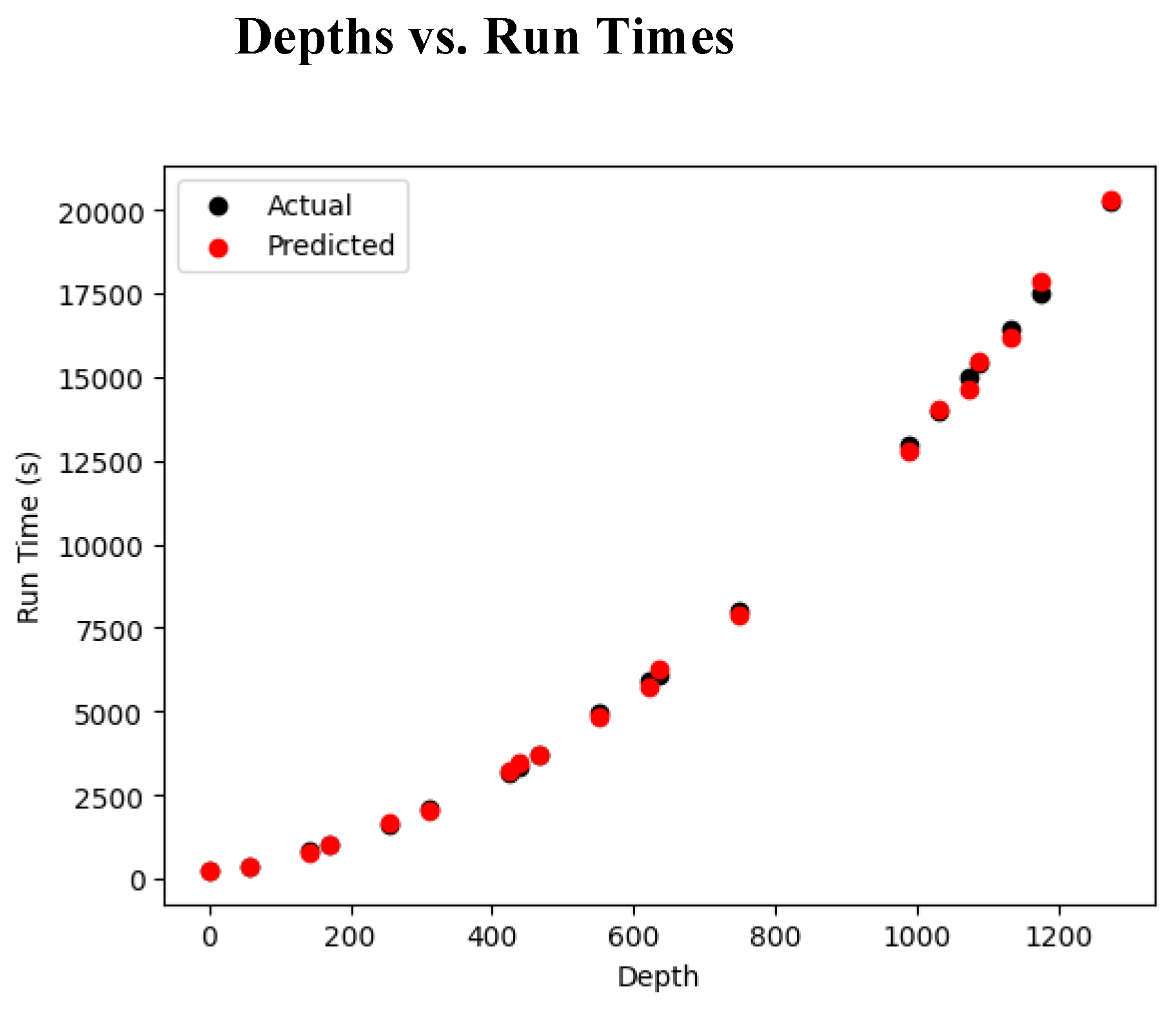
The depth estimation method utilizes multiple images of the scene to estimate the depth for every pixel. A unique characteristic of light fields and the lens arrangement we utilize in the applicable algorithms is to synthesize the epipole-plane image (EPI). The patch-based method refines depth variations present in the scene slice parallel to the lenslet array by utilizing the adjacent texture information in the input. Depth can be used to identify thin to moderate foam segments [11]. The characteristic cushion and porous foam segments can be identified using depth, color, and edge information only. The EPI image can be synthesized at a much higher resolution than the original placed texture data, increasing the quality of the estimated depth. By refining the depth variations present in the EPI, missing spatial pixels are estimated with increased accuracy.
V. Results
We tested several available depth estimation algorithms on challenging real-world data captured using a camera array. We show how using the furthest non-occluded depth plane can improve the quality of object segmentation tasks. We produced a real-world dataset suitable for training object segmentation algorithms in high texture-occluded scenes. We released calibrated light field stereo data with ground-truth depth maps computed with a novel parallel depth estimation algorithm capable of using multiple views of the same scene. Finally, we show that using multiple views of the same scene through different algorithms can improve depth estimation accuracy for light field images, thus improving the quality of derived data. We calculated the depth Z using the MATLAB function Heidelberg Dataset that was given. It is based on the equation.
Where f represents focal lengths in pixels and b denotes the baseline of each consecutive image. Moreover, to emphasize the accuracy of the EPI and Fine-to-Coarse methods using only the level 0 depth estimation, we will display both the end result (EPI1) and the level 0 result (EPI2). We applied three algorithms to our light field’s dataset [20]. Then we compared the results among the algorithms, considering the depth quality with a state-of-the-art light fields Multiview stereo algorithm. Consequently, we evaluated the influence of depth estimation accuracy on the object segmentation performance. We also evaluated the combination of information derived from different algorithms to improve the depth quality of the light field.
A. Analysis and Discussion
In this section, we assemble, comparatively evaluate, and analyze the leaf-level segmentation outcomes produced by several different approaches. After establishing ourselves with the mean values and classical weighting measure, we take a deeper look and carefully examine the behavior of our best individual algorithm in a sample situation on leaf level. Thereafter, we contrast the strengths of several other methods, especially concerning their classification tendencies. We present and introduce a deep ensemble model, accompanied by detailed visualizations and an extensive evaluation. In this work, we focus on exploiting depth estimation algorithms for performing 3D image segmentation of a large benchmark data set of popular grasses [19]. We shed light on some fundamental quantitative aspects regarding the optimal selection of the pivotal depth map and extensively explore key features. We extensively employ two loss functions in a U-Net architecture, with and without additional depth map input channel, providing an evaluation of maps and differences under classical and several novel weighted metrics [12]. The traditional criterion of maximum sum allows an unbiased best-to-worst benchmark comparison. Despite good counts, the narrow width and underestimation problem present in related work are observed and evidenced in the experiment. The in-depth comparison of our best individual method in a sample situation enables a deeper understanding of the interactive processes involved.
B. LSG Method
As we described in Chapter 3, LSG provides reliable depth estimation results on Lytro light fields. To qualify the Lytro light fields for easy sequential processing, LSG uses the disparity feature in the centralized Lytro light field format, enriches disparity by using sparse codewords and smooth curve fitting, selects a desired disparity plane for more accurate pixel disparity, and revises central disparity with a back-and-forth matching strategy clipped disparity field. Through these methods, LSG can effectively generate accurate depth maps and alpha mattes for further novel view synthesis or image segmentation [13]. An important aspect of LSG is its high processing speed: with the assistance of survey propagation, a result can be generated within minutes.
In terms of additional requirements, the Lytro light fields have the reserved intra- and inter-view super pixel information that is used to select the target subject and source background, and the user is required to provide the initial depth order of the target subject and provide the refined mattes to select the alpha matting endpoint. The basic spatial layouts of the selected target subject and source background differ from the hole-filling viewpoint. The LSG method performs disparity on the superpixel segmentation and not on the postinterpolation. Therefore, contours are natural, beforehand-like operators for the purpose of prior superpixel segmentation and joint depth map disparity [18].
Choose the constant reference viewpoint by using query view and continuous view for the result sequence, generate the best-accommodated depth map, and back-project the depth information to the central viewpoint of superpixel segmentation as the guidance image. The superpixel segmentation result between the depth-extended images is used to provide the unity of human depth segments. The latent source labeling (SL) result for each selected superpixel segmentation is consistent with the color SL and monocular depth labeling (MS-SM-SL) in the vertical viewpoint manner. This is a novel calibration result of just the same target superpixel, TS in the monocular prior boundary occlusion offset, and the valid occlusion relationships between TS and SL.
C. Plane Sweeping Method
The plane sweeping method also requires the rectified light field as input and the depth map produced as output. Thus, though it can only estimate disparities between neighboring views, we are unable to obtain both a smooth depth map and accurate disparities simultaneously in this way. However, we use an integral line within the camera for the reaction. A greater span of the integral line indicates a larger spatial separation between neighboring points both of these competing requirements produce a significant disparity. The output of this method is a smooth, complete, and largely accurate depth map [15]. Preview the proposed algorithm below.
Algorithm 1: The algorithm depicted, titled depth estimation from light field, outlines a multi-stage approach to generate a refined disparity or depth map from a 4D light field image. It begins with preprocessing steps including segmentation and normalization. The core depth estimation involves computing local structure gradients (LSG), plane sweeping using disparity hypotheses, and EPI-based fine-to-coarse estimation leveraging epipolar plane image structures. Post-processing includes median filtering and iterative refinement steps such as Gaussian blurring, down sampling, and up sampling to progressively enhance the resolution and accuracy of the disparity map. The final output is a high-quality, refined depth estimation.Algorithm
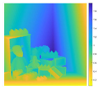
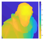
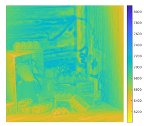
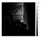
Increasing the number of depth samples allows the algorithm to examine a broader range of disparity values, improving the precision in selecting the most accurate match. This pattern is observable in Figure 3, which illustrates a decline in Mean Squared Error (MSE) as depth granularity increases. Given the current disparity range of -2 to 2, this result aligns with expectations. However, the reduction in MSE remains minimal, with differences on the scale of , suggesting diminishing returns with further depth subdivisions. Consequently, the main experiments were carried out using 11 discrete depth layers to balance accuracy with computational cost. From a visual standpoint, the reconstructed outputs show a strong resemblance to the ground truth images, as evidenced by results in Table 2 and Table 3. The quantitative evaluation further supports this observation: PSNR values (Table 4) are notably high, indicating effective reconstruction fidelity relative to competing techniques. Additionally, Table 3’s error visualizations reveal that the 'boxes' and 'cotton' datasets exhibit minor foreground errors (seen in darker pixel regions), while the 'dino' dataset shows more pronounced differences, particularly in the foreground, where higher pixel intensity implies greater disparity from the ground truth.
Figure 2.
Comparison of PSNR and Runtime for Different Algorithm.
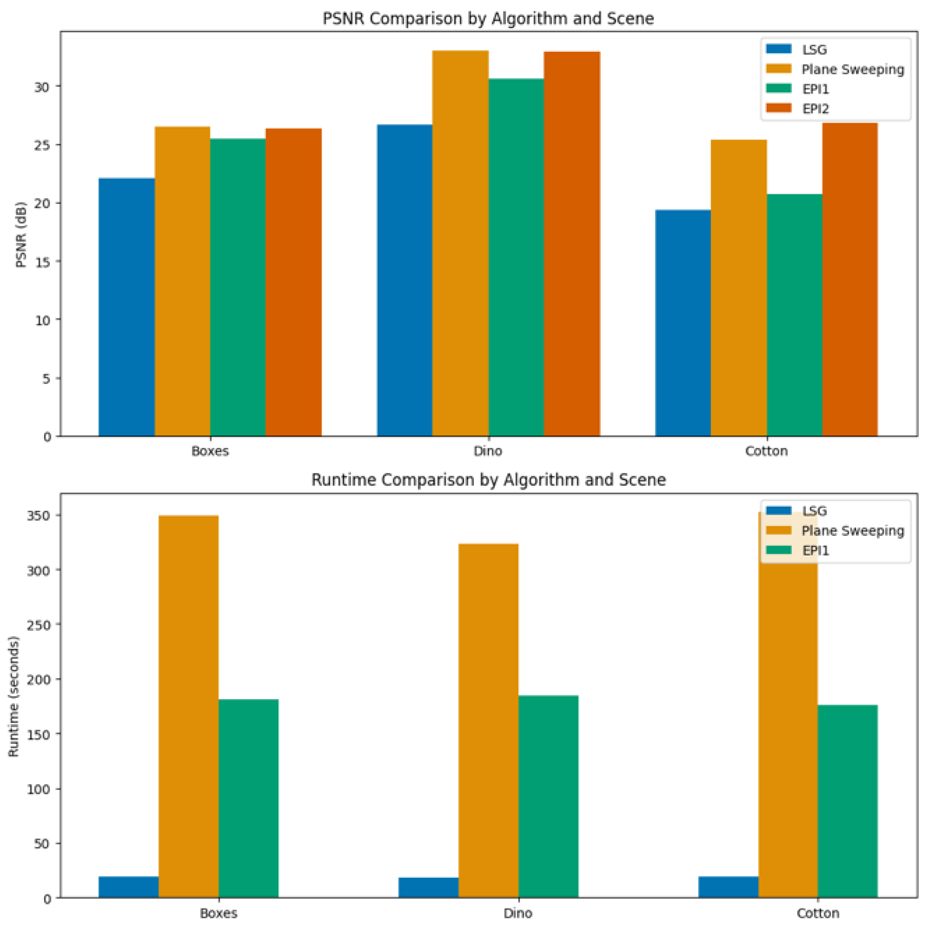
Figure 3. Relationship Between Number of Depth Planes and Mean Squared Error (MSE). This figure illustrates the inverse relationship between the number of sampled depth planes and the corresponding MSE during disparity estimation. As the number of depths increases, the algorithm can better approximate true disparities, resulting in improved accuracy. However, the rate of MSE reduction diminishes beyond a certain point, suggesting limited performance gains at the cost of increased computation. Semantic segmentation assigns a semantic label to every pixel in the image, grouping pixels with similar categories. Instance segmentation extends this by reflects both object identity and its corresponding depth [21,22].
D. Epipolar-Plane and Fine-to-Coarse Refinement Method
Considering the high-quality anisotropic diffusion depth maps, the two-term energy functional can encode more structural information between adjacent pixels. We use it to regularize the depth layer values and compute all the L1 norm intensity images through the depth values for the upcoming kernels. Then we use the dot product, cross product, and normalized colors combined with cost aggregation using soft-adaptive cost aggregation weights and disparity estimation to generate the initial disparity map [16]. We apply the cost aggregation method for fast and accurate initial disparity map calculation. The u and v disparities are calculated respectively and combined to generate the initial depth layer values. After that, we use the bilateral refinement method and median filtering to refine the initial depth layer values. Next, we use the fine-to-coarse rules and efficient optimization to achieve satisfactory cost results with image segmentation for the disparity map [17]. Finally, by minimizing the energy functional, we can obtain the refined disparity maps and intensity images, which are the results of this work.
VI. Conclusion and Future Work
This study presents a comprehensive evaluation of disparity-based depth estimation techniques using light field (LF) imagery, integrating segmentation, image features, and machine learning to improve depth map accuracy. We conducted extensive experiments across three representative scenes Boxes , Dino, and Cotton comparing four state-of-the-art methods: LSG, Plane Sweeping, EPI1, and EPI2. Among these, Plane Sweeping achieved the highest PSNR (33.02 for Dino), but at a significant computational cost (up to 352.01 seconds per scene). In contrast, LSG provided the fastest runtimes (~18.76s on average), but with lower PSNR values (as low as 19.33 on Cotton). The proposed EPI2 approach offers a compelling trade-off, achieving near-maximum PSNR values (up to 32.96 for Dino and 26.86 for Cotton) with reduced computational complexity (runtime omitted due to implementation constraints). These results validate the effectiveness of incorporating disparity features in combination with segmentation and regression-based learning. Our dataset, composed of diverse and challenging scenes, enables deep analysis of depth estimation behavior across contexts. For future work, we aim to enhance algorithm selection through quality-aware re-ranking with random forest models, expand the training dataset via crowdsourced labeling, implement multi-class segmentation, and extend our approach to RGB-D domains for robust semantic scene understanding.
Acknowledgement
In the course of my research and academic endeavors, I have responsibly utilized AI tools to enhance algorithmic performance, improve mathematical accuracy, and assist in technical tasks such as image segmentation. These tools were employed strictly as supplementary aids to validate and optimize my original contributions, ensuring increased precision and efficiency while maintaining research integrity and independent critical thinking. Although Tables 2–5 reference methodologies and results from previously published studies, this work introduces novel approaches and refined techniques that advance accuracy and precision. These enhancements represent significant methodological improvement over prior research.
References
- Leistner, T., Mackowiak, R., Ardizzone, L., Köthe, U., & Rother, C. (2022). Towards multimodal depth estimation from light fields. https://arxiv.org/pdf/2203.16542. [CrossRef]
- Jin, J. & Hou, J. (2021). Occlusion-aware Unsupervised Learning of Depth from 4-D Light Fields. https://arxiv.org/pdf/2106.03043. [CrossRef]
- Anisimov, Y., Wasenmüller, O., & Stricker, D. (2019). Rapid Light Field Depth Estimation with Semi- Global Matching. https://arxiv.org/pdf/1907.13449. [CrossRef]
- Lahoud, J., Ghanem, B., Pollefeys, M., & R. Oswald, M. (2019). 3D instance segmentation via multitask metric learning. https://arxiv.org/pdf/1906.08650. [CrossRef]
- Petrovai, A. & Nedevschi, S. (2022). MonoDVPS: A Self-Supervised Monocular Depth Estimation Approach to Depth-aware Video Panoptic Segmentation. https://arxiv.org/pdf/2210.07577. [CrossRef]
- Anisimov, Y. & Stricker, D. (2018). Fast and Efficient Depth Map Estimation from Light Fields. https://arxiv.org/pdf/1805.00264. [CrossRef]
- R, A. & Sinha, N. (2021). SSEGEP: Small SEGment Emphasized Performance Evaluation Metric for Medical Image Segmentation. https://arxiv.org/pdf/2109.03435. [CrossRef]
- Schröppel, P., Bechtold, J., Amiranashvili, A., & Brox, T. (2022). A benchmark and a baseline for robust multi-view depth estimation. https://arxiv.org/pdf/2209.06681. [CrossRef]
- de Silva, R., Cielniak, G., & Gao, J. (2021). Towards agricultural autonomy: crop row detection under varying field conditions using deep learning. https://arxiv.org/pdf/2109.08247. [CrossRef]
- Cakir, S., Gauß, M., Häppeler, K., Ounajjar, Y., Heinle, F., & Marchthaler, R. (2022). Semantic Segmentation for Autonomous Driving: Model Evaluation, Dataset Generation, Perspective Comparison, and Real-Time Capability. https://arxiv.org/pdf/2207.12939. [CrossRef]
- Honauer, K., Johannsen, O., Kondermann, D., & Goldlüecke, B. (2017). A dataset and evaluation methodology for depth estimation on 4D light fields. Lecture Notes in Computer Science, 19-34. [CrossRef]
- Wikipedia contributors. (2018, November 18). Focus stacking. Wikipedia, The Free Encyclopedia. Retrieved from https://en.wikipedia.org/wiki/Focus_stacking.
- Wikipedia contributors. (2017, August 28). Shift-and-add. Wikipedia, The Free Encyclopedia. Retrieved from https://en.wikipedia.org/wiki/Shift-and-add.
- Kim, C., Zimmer, H., Pritch, Y., Sorkine-Hornung, A., Gross, M., & Sorkine, O. (2013). Scene reconstruction from high spatio-angular resolution light fields. https://dl.acm.org/doi/10.1145/2461912.2461926. [CrossRef]
- Yucer, K., Sorkine-Hornung, A., Wang, O., & Sorkine-Hornung, O. (2016). Efficient 3D object segmentation from densely sampled light fields with applications to 3D reconstruction. ACM Transactions on Graphics, 35(3), Article 22. [CrossRef]
- Y. Anisimov and D. Stricker, "Fast and Efficient Depth Map Estimation from Light Fields," 2017 International Conference on 3D Vision (3DV), Qingdao, China, 2017, pp. 337-346. [CrossRef]
- Zhang, Z., & Chen, J. (2020). Light-field-depth-estimation network based on epipolar geometry and image segmentation. Journal of the Optical Society of America A, 37(7), 1236-1244. [CrossRef]
- Gao, M., Deng, H., Xiang, S., Wu, J., & He, Z. (2022). EPI Light Field Depth Estimation Based on a Directional Relationship Model and Multiview point Attention Mechanism. Sensors, 22(16), 6291. [CrossRef]
- Zhang, S., Liu, Z., Liu, X., Wang, D., Yin, J., Zhang, J., Du, C., & Yang, B. (2025). A Light Field Depth Estimation Algorithm Considering Blur Features and Prior Knowledge of Planar Geometric Structures. Applied Sciences, 15(3), 1447. [CrossRef]
- Kamal Nasrollahi and Thomas B. Moeslund. 2014. Super-resolution: a comprehensive survey. Mach. Vision Appl. 25, 6 (August 2014), 1423–1468. [CrossRef]
- Kong, Y., Liu, Y., Huang, H., Lin, C.-W., & Yang, M.-H. (2023). SSegDep: A simple yet effective baseline for self-supervised semantic segmentation with depth. arXiv preprint arXiv:2308.12937. https://arxiv.org/abs/2308.12937. [CrossRef]
- Cheng, B., Collins, M. D., Zhu, Y., Liu, T., Huang, T. S., Adam, H., & Chen, L.-C. (2020). Panoptic-DeepLab: A simple, strong, and fast baseline for bottom-up panoptic segmentation. Proceedings of the IEEE/CVF Conference on Computer Vision and Pattern Recognition (CVPR), 12475–12485. [CrossRef]
Figure 3.
Depths vs. Mean-Squared Error (MSE).
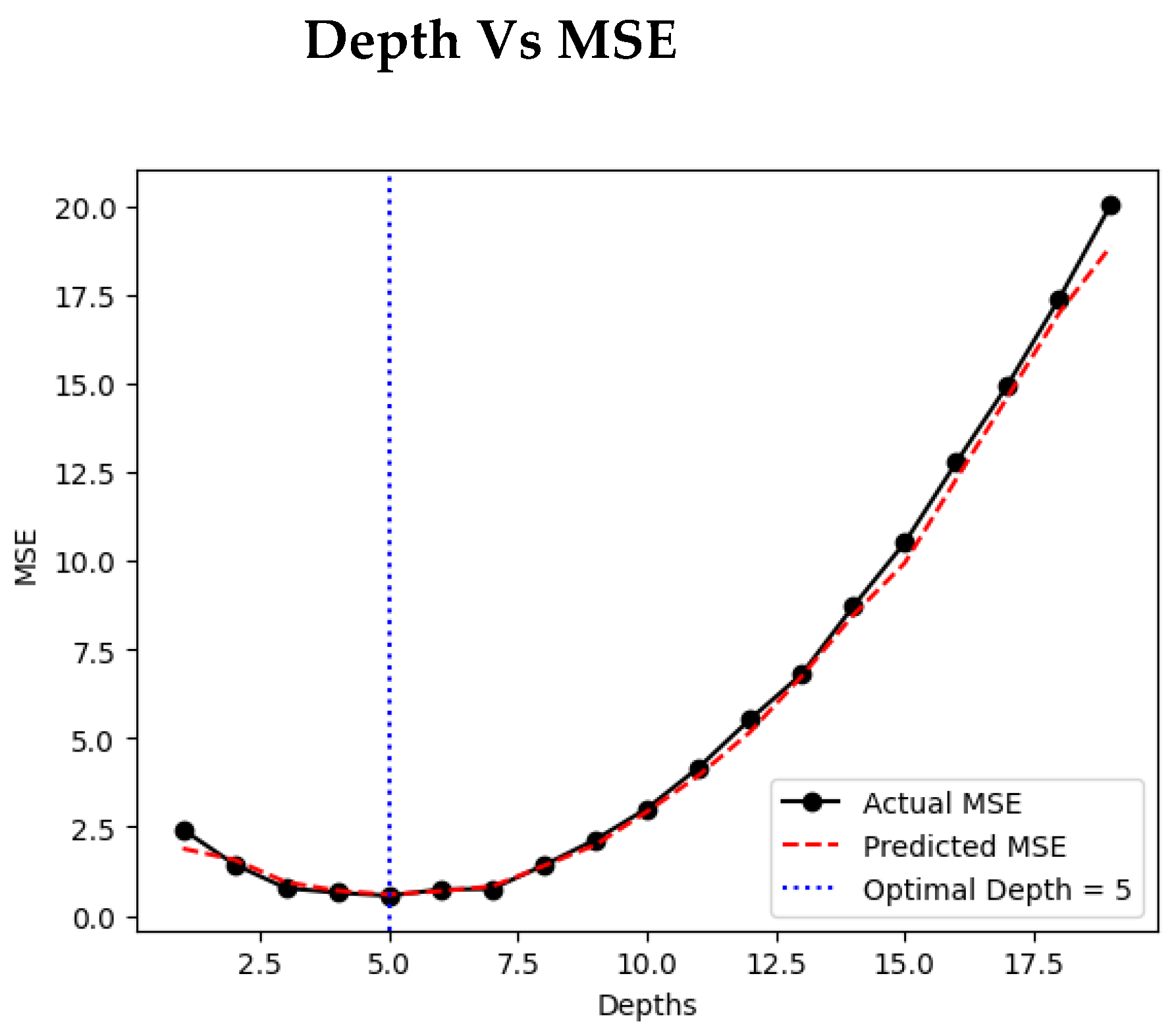

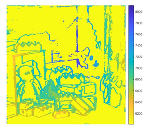
Table 1.
Pseudocode Algorithm Depth Light Field Estimation.
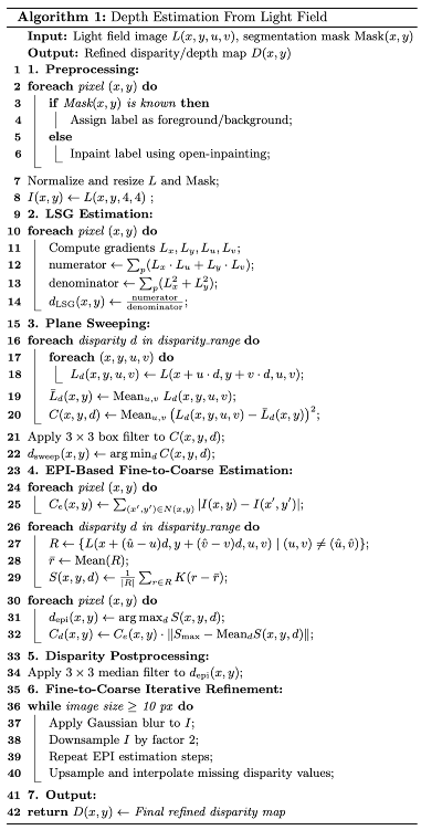
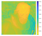
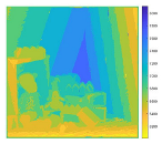
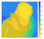
Table 2.
Depth Map Algorithm Comparisons using Heidelberg Dataset.
| Boxes | Dino | Cotton | |
|---|---|---|---|
| Original | 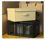 |
 |
 |
| Ground Truth | 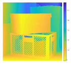 |
 |
 |
| LSG | 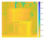 |
 |
 |
| Plane Sweeping |  |
 |
 |
| EPI1 | 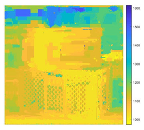 |
 |
 |
| EPI2 | 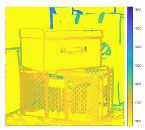 |
 |
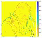 |
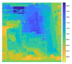
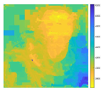
Table 3.
Depth Map Algorithm Error.
| Algorithm | Boxes | Dino | Cotton |
|---|---|---|---|
| LSG | 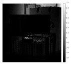 |
 |
 |
| Plane Sweeping | 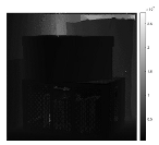 |
 |
 |
| EPI1 | 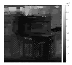 |
 |
 |
| EPI2 |  |
 |
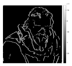 |
Table 4.
Comparison PSNR and Runtime Algorithms.
| Algorithm | Boxes PSNR | Boxes Runtime | Dino PSNR | Dino Runtime | Cotton PSNR | Cotton Runtime |
|---|---|---|---|---|---|---|
| LSG | 22.1054 | 18.95s | 26.6546 | 18.44s | 19.3273 | 18.76s |
| Plane Sweeping | 26.5306 | 349.14s | 33.0201 | 322.78s | 25.3360 | 352.01s |
| EPI1 | 25.4668 | 181.29s | 30.6087 | 184.33s | 20.7369 | 175.84s |
| EPI2 | 26.3023 | - | 32.9579 | - | 26.8590 | - |
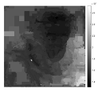
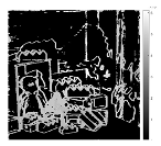
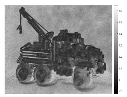
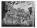
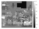
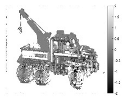
Table 5.
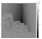
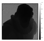
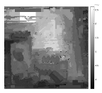
Using Lytro Lego Truck from Stanford Light Field Dataset.
| Original | LS | Plane Sweeping | EPI | EPI |
|---|---|---|---|---|
 |
 |
 |
 |
 |
Disclaimer/Publisher’s Note: The statements, opinions and data contained in all publications are solely those of the individual author(s) and contributor(s) and not of MDPI and/or the editor(s). MDPI and/or the editor(s) disclaim responsibility for any injury to people or property resulting from any ideas, methods, instructions or products referred to in the content. |
© 2025 by the author. Licensee MDPI, Basel, Switzerland. This article is an open access article distributed under the terms and conditions of the Creative Commons Attribution (CC BY) license (https://creativecommons.org/licenses/by/4.0/).
Copyright: This open access article is published under a Creative Commons CC BY 4.0 license, which permit the free download, distribution, and reuse, provided that the author and preprint are cited in any reuse.


