
Submitted:
01 June 2025
Posted:
04 June 2025
You are already at the latest version
Abstract
The main contribution is to provide machine learning and quality practitioners with a complete and practical method to estimate the lower bound of the intrinsic kappa coefficient and accuracy. Kappa statistic is one of the most used methods to evaluate the effectiveness of quality inspections based on attributive characteristics. Kappa and accuracy are also extensively used for classification problems in machine learning. This article develops exact and approximate methods to estimate the lower bound of kappa's "intrinsic" value for any number of categories. In addition, two methods (exact and approximate) are provided to estimate the accuracy lower bound for machine learning practitioners who prefer this performance metric. For the intrinsic kappa coefficient and accuracy, the results showed that the approximate methods’ estimations are very close to those from the exact method for a wide range of sample sizes and misclassified instances, indicating that the approximate can be used for any number of categories. Additionally, real-life examples illustrate the use of the method for practitioners.
Keywords:
kappa coefficient
; confidence limit
; machine learning
; accuracy
; classification problems
1. Introduction
The Kappa coefficient has recently gained researchers’ interest for its use as a performance metric in machine-learning classification problems [1]. However, due to its intuitive meaning, accuracy is still expected to be a complementary measure of kappa within the same works [2,3,4,5,6,7].
Sanchez-Marquez et al. [8] show that kappa is also extensively used for quality inspections of attributive characteristics, which is a classification problem [9,10,11,12,13,14]. In this context, the degree of assessment agreement is the same concept as accuracy in machine learning; both measures are the same statistic. Sanchez-Marquez et al. [8] developed the “intrinsic” kappa coefficient, which is robust against imbalanced samples compared to the traditional kappa coefficient that proved biased under such conditions.
Kappa and accuracy measures are also used in any field with a classification problem [15,16,17,18,19].
Researchers and practitioners can also use other metrics to evaluate classifier performance, such as G-Mean and curve ROC, each offering benefits and limitations. This paper does not aim to compare different available metrics with the one developed here. Instead, it focuses on generalising the intrinsic kappa coefficient, a metric whose application in machine learning classifiers has recently gained attention, making it usable for any number of categories. Furthermore, most current metrics for classifiers, such as G-Mean or curve ROC, are limited to two categories. In contrast, the metric developed in this work is designed to work with any number of categories.
Like other statistics, kappa has its variance; therefore, using its point estimate is incorrect since the effect of the sample size should be considered. The literature has addressed the necessity of estimating kappa’s confidence intervals or lower bounds using different approaches [8,20,21,22]. Other limitations of the kappa coefficient have been discussed [20,21,23,24,25], such as bias due to expected agreement, the challenges of using multiple raters, and the application of weighted scales. However, despite these advancements, some gaps remain unsolved. Available works using kappa still have two main problems. The first problem is that the coefficient depends on the sample bias, e.g., when samples are not balanced over the different categories, the traditional kappa coefficient [20,21,23,24,25] depends on the percentage of instances of each category [8], also called as prevalence. This characteristic of the traditional kappa coefficient is a drawback since we could change the result by only adjusting the sample prevalence without improving the classification system’s performance. The other problem is that these traditional kappa statistics are based on asymptotic approximations used without analysing the performance for small samples or developing an alternate exact method.
Donner & Rotondi [22] address the sample size problem, while Sanchez-Marquez et al. [8] also develop an exact method and derive expressions for the intrinsic kappa coefficient. As Sanchez-Marquez et al. mentions, the point estimate of the intrinsic kappa coefficient does not depend on the prevalence of the sample, which is the main drawback of the traditional kappa coefficient. Sanchez-Marquez et al.’s method [8] is especially interesting for machine learning research and applications. Researchers and practitioners must train the models using available data, which only sometimes contains balanced samples for the different categories. However, both papers only apply to binary applications, e.g., applications with two categories. In addition, Donner & Rotondi [22] provide tables for selecting the best sample size for each case, which is a limitation for the generalisation of the method. Sanchez-Marquez et al. [8] use an exact method that needs several expressions and the F distribution, thus losing the simplicity of the traditional methods based on asymptotic approximations.
This paper addresses the gaps mentioned above by developing generalised exact and approximate methods for estimating the lower bound of the intrinsic kappa coefficient and accuracy for any number of categories (NC). The results showed that the approximate methods performed well even for tiny sample sizes and low rates of misclassified instances.
The next sections are organised as follows:
- -
- Section 2, titled “On the generalisation of the intrinsic kappa coefficient for any number of categories”, derives exact and approximate generalised expressions for estimating the lower bound of the intrinsic kappa coefficient and accuracy.
- -
- Section 3 shows the comparison results between the exact and approximate methods. It also provides insights into the effect of the number of categories on estimating the intrinsic kappa coefficient.
- -
- Section 4 discusses if the main objectives set up in the introduction section have been met. It also discusses possible limitations and future research.
- -
- Section 5 shows the application of the method using actual data.
2. Materials and Methods
Sanchez-Marquez et al. [8] derived an intrinsic kappa coefficient for dichotomous categories, with its point estimate expressed as
where is the point estimate of the intrinsic kappa coefficient, is the type-I error (the proportion of non-defective units misclassified), and is the type-II error (the proportion of defective units misclassified). Significantly, this coefficient does not depend on the percentage of instances of each category, giving us a robust measure unaffected by class prevalence. Regretfully, it can be applied only to dichotomous problems. This paper aims to develop a generalised intrinsic kappa coefficient applicable to problems with any number of categories.
In Figure 1, the confusion matrix is contained inside the bold square. The labels A, B ..., and NC represent the categories used to classify each instance or unit. Every instance is assigned a label from one of these categories. The labelling process occurs twice. The first labelling is conducted beforehand and is known as the ’known standard.’ The initial label serves as a reference or benchmark to train and validate the classification system, whether it involves a machine learning algorithm or a group of human raters. The classification system itself performs the second labelling. Comparing these two labels reveals the system’s performance. In this context, performance metrics such as the kappa coefficient quantitatively measure the system’s classification accuracy. In this matrix and the following lines formulae, m represents the number of repetitions a particular object or instance is evaluated and classified. Therefore, m only makes sense in the context of quality inspections but not in machine learning since every time an instance is classified, it will be classified as belonging to the same category; thus, in machine learning, m = 1. The notation P(i/j) represents the probability or percentage of instances or units classified as belonging to class i when they belong to j, with i and j ranging from A to NC. Similarly, Xi/j indicates the number of instances or units classified in this manner. It is important to note that instances are correctly classified along the matrix diagonal i = j. The number of units known to belong to class i is denoted by ni; finally, N represents the total number of instances.
Figure 1 shows a confusion matrix for generalising the intrinsic kappa coefficient first developed by Sanchez-Marquez et al. [8]. For simplification, NC stands for the number of categories and the name of the last category. According to Sanchez-Marquez et al. [8], for deriving the intrinsic kappa coefficient, which should not depend on the proportion of units belonging to each category, we must set up the sample as balanced and assume the hypothesis that we will obtain an expression that does not depend on the proportion of units in each category. However, this does not imply that the sample must be balanced. Instead, this approach leads to a kappa coefficient expression independent of sample prevalence, yielding the intrinsic kappa coefficient. As noted earlier, Sanchez-Marquez et al. [8] were the first to derive the intrinsic kappa coefficient for dichotomous problems, employing similar fundamental concepts and methodology. Once the expression for the intrinsic kappa point estimate is derived, we must check if the initial hypothesis is met and then account for the different sample sizes in each category using kappa’s lower bound computed by the F-statistic level of significance for the exact method or the standard error for the approximate one. As explained by Sanchez-Marquez et al. [8], by forcing the same number of instances in all categories, we obtain a coefficient that does not depend on the prevalence so that it is the value that a balanced experiment would obtain, which is the intrinsic value of kappa. The intrinsic kappa coefficient shows how well the system (or the classifier in machine learning) classifies the instances regardless of the proportion of units in each category. It does not happen with the traditional kappa coefficient, which would change its value without changing the classifier performance by changing the proportion of units belonging to each category. Therefore, by using the expressions of the intrinsic kappa coefficient, we obtain the same result as with the traditional kappa coefficient with a balanced sample but without the need for the sample to be balanced. Once the expression of the point estimate of the intrinsic value of the kappa coefficient has been obtained, it is necessary to consider the estimation error due to the sample size by expressing a confidence interval or limit.
In Figure 1, the conditional proportions are shown on the top of each cell. Every cell shows a proportion on the top and a count below. For example, the first cell of the matrix in the upper left-hand corner contains the proportion of instances evaluated as belonging to category A that are known to belong to A, so P(A/A). It also contains the count of instances, which, in this cell, is the number of instances evaluated as A when it is known they belong to A. Therefore, all cells contain the conditional proportion by column and their corresponding conditional count. The additional cells outside the confusion matrix (outside the bold square) also show the proportion on the top and the count below, except for the lower right-hand corner, which only contains the total count since the overall proportion is one. As mentioned above, the confusion matrix shown in Figure 1 is built according to the hypothesis that assuming the number of instances belonging to all categories is equal (nA = nB = … = nNC) will allow us to derive the intrinsic kappa coefficient.
According to Everitt [23], the kappa coefficient is defined as
where is the proportion of observed agreements, and is the proportion of expected agreements (which can also be understood as agreements obtained by chance). The observed agreements denoted as Xo, will be on the diagonal of the confusion matrix, representing the well-classified instances. The off-diagonal counts are the misclassified ones. It is the idea behind the accuracy, which, along with kappa, is one of the most widely used performance metrics in machine learning. For those interested in a deeper understanding, foundational literature ([23]) delves into the definition and application of the kappa coefficient. The confusion matrix can be summarised using the proportion of well-classified instances. Therefore, and .
Looking at Figure 1, we can see that the sum of all conditional proportions inside the confusion matrix is NC since conditional proportions on each column sum up to one. Therefore,
Substituting (3) in (1) we obtain
The initial hypothesis has been confirmed since, in Eq. (4), the point estimate of kappa does not depend on the prevalence. Therefore, Eq. (4) and Eq. (2) compute the point estimate of the intrinsic kappa coefficient.
It is exciting and intuitive that the intrinsic kappa statistic that considers the probability of classifying well by chance only depends on the number of categories. Figure 2 shows the behaviour of for a typical accuracy level—. It shows that the intrinsic kappa coefficient is penalised when NC is minimum (NC = 2). Thus, is also the minimum. The larger the NC, the greater the . The behaviour shown in Figure 2 reflects that the larger the number of categories, the more difficult it is to classify well by chance, which is coherent with the definition of the kappa coefficient. Therefore, the intrinsic kappa coefficient considers the probability of classifying well by chance, and it depends on the number of categories, which is more coherent than what happens with the traditional kappa coefficient. The traditional coefficient reflects that classifying well by chance also depends on the proportion of instances belonging to each category [8]. It means that it is more coherent that the probability of classifying a particular unit or instance well depends only on the number of categories and not on the proportion of units in the sample belonging to each category. The latter does not make sense. Therefore, the intrinsic kappa coefficient better reflects how the system (human or automated) classifies itself than the traditional coefficient.
It is well-known that , therefore Eq. (4) must meet this essential characteristi . It means that when , .
We can derive the above conclusion directly from Eq. (4), which means that it applies to any number of categories:
Sánchez-Marquez et al. [8] derived the following equation for the case of two categories:
where is the proportion of wrong-classified non-defective instances, and is the proportion of wrong-classified defective instances.
If Eq. (5) is a particular case of Eq. (4), Eq. (5) should appear from Eq. (4) if we express Eq. (4) as a function of and . Let us check it.
For two categories and expressing it in terms of and , we have that
From Eq. (4),
, that for two categories and expressing it in terms of α and β, we arrive at
Therefore, we have confirmed that Eq. (5) and (4) are equivalent for NC = 2.
As mentioned in the literature [8], it is essential not to use the point estimate, thus considering the sample size. The following lines derive expressions to estimate the confidence lower bound of the intrinsic kappa coefficient and the accuracy using exact and approximate methods.
2.1. Exact Confidence Lower Bound of the Intrinsic Kappa Coefficient Accuracy for Any Number of Categories
As mentioned above, is the proportion of the well-classified instances; thus, it is a binomial statistic. Therefore, we can compute the exact confidence lower bound for k based on the F distribution [26] [27]:
where kLB is the confidence lower bound of the intrinsic kappa coefficient and is the confidence lower bound of the accuracy.
In Eq. (6):
where:
- -
- -
- -
- is the number of wrong classifications.
- -
- is the total number of instances.
- -
- is the value of the inverse F function for a significance level of α, and and degrees of freedom.
It should be remarked that Eq. (7) computes the accuracy lower bound using the number of failures or wrong-classified instances [26], which are the instances outside the diagonal elements of the confusion matrix. Therefore, to account for the estimation error caused by the sample size, practitioners and researchers who prefer accuracy as a performance metric must use this expression as a metric performance instead of using the point estimate, which is the common practice so far.
To compute the lower bound of the intrinsic kappa for one category (category i), we must build a confusion matrix for two categories. One category would be that we are interested in computing the kappa lower bound, and the other would summarise the ratings of the rest of the categories. Once we have constructed this two-way table, we apply the same concept as that of Eq. (6) and (7) but for two categories:
where:
where:
- -
- is the accuracy lower bound for the i category.
- -
- .
- -
- .
- -
- is the number of wrong-classified instances.
- -
- N is the total number of instances.
- -
- is the value of the inverse F function for a significance of α, and and degrees of freedom.
- -
- is the number of well-classified instances that belong to the i category.
- -
- is the number of instances that do not belong to the i-category and are classified as not belonging to that category.
As with the overall performance, to compute the accuracy lower bound of one category, practitioners and researchers must build a two-way table as mentioned above and use Eq. (9) instead of the point estimate.
Agresti & Coull [26] showed that approximate methods perform better than exact ones for binominal variables. It is worth deriving approximate methods for the estimation of confidence limits, not only due to their precision but also due to their simplicity [26], which allows practitioners and researchers to implement them using basic software packages such as Excel [27] [28]. Therefore, in the following lines, we will derive approximate Clopper-Pearson expressions [29] to approximate the lower bound of the intrinsic kappa coefficient, which will be tested in the results section. Since accuracy is a simple binomial variable, we can rely on Agresti & Coull’s results [26] to use its approximate expressions, which will also be derived in the next section.
2.2. Approximate Lower Bound of the Intrinsic Kappa Coefficient and Accuracy for any Number of Categories
To derive asymptotic approximate expressions for confidence limits of any statistic, we must start by deriving the variance of the statistic point estimate. Therefore, from Eq. (4):
As :
According to Clopper & Pearson [29] and Agresti & Coull [26], from the statistic variance, we can construct the approximate confidence interval (CI) for p by inverting the Wald test for p.
From the inverted hypothesis test:
that uses the z statistic ,
H0: p = p0 vs Ha: p ≠ p0
we can derive the inverted confidence interval [26], which is:
It is well-known that . Therefore,
However, since we do not usually have the population parameter p, the approximate CI is commonly calculated using an estimator, which is the parameter point estimate . Therefore, the resulting Wald interval for p, which, according to Agresti & Coull [26], is one of the first parameter intervals ever derived is:
If we are interested in one bound, the expressions are:
for the lower and upper bound, respectively.
It is well-known that, based on the central limit theorem (CLT), Wald’s hypothesis test and its derived interval have been generalised as a method to define normal approximations for CIs of any statistical parameter. This generalisation can be expressed as:
where is the parameter of interest and its estimator.
The expressions for one-bound estimations are:
Therefore, applying Wald’s generalisation for the intrinsic kappa coefficient from (15), we obtain
is defined in Eq. (10), which leads us to
Like what happens with the p’s CI, usually is not known, so we need to use an estimator for . Like in Wald’s interval, the most obvious option is using ’s point estimate; thus,
where is the value of the inverse standard normal distribution function for α significance level; ; N is the total sample size.
Agresti & Coull [26] showed that the approximate Wald’s adjusted method can improve the results of the original Wald’s method by adding two failures and four instances to the point estimate. It means that in Eq. (18).
The following section will confirm that Eq. (18) approximates the value of kLB well for a wide range of sample sizes and accuracy rates. It will also compare results from adjusted and non-adjusted approximate lower bound.
Since the accuracy is a binomial statistic, based on Agresti and Coull’s results [26], we must apply the adjusted Wald’s approximate method for the proportion statistic. Therefore, for our purpose, we will have that
where . Notice that the point estimate must be adjusted by adding two counts to the smallest proportion, the number of failures or wrong-classified instances [26].
3. Results
This section presents the results of comparing exact and approximate methods for a wide range of sample sizes and accuracy levels, as well as for NC = 2, 3, and 10.
As for the binomial p parameter, we expect the approximate and exact methods to obtain similar results in the lower bound, thus validating that the approximate method can be used to estimate kLB.
Table 1, Table 3 and Table 5 are built using Eq. (4) and Eq. (19) without adjusting . Therefore, , where X is the total number of failures or wrong-classified instances found outside the confusion matrix’s diagonal. N is the total amount of instances, including repetitions—if any—in the context of quality inspections. In machine learning applications, we just talk about instances without repetitions. Table 2, Table 4 and Table 6 use the adjusted point estimate for the variance in Eq. (19), thus . N is the total number of machine learning or quality assessments in the context of quality inspections. Failures are the wrong-classified instances (counts outside the confusion matrix diagonal). Relative error is defined as
Looking at all tables, we can conclude that, although the kappa coefficient is typically expressed using two decimals, we must go to the third decimal (or beyond) to see discrepancies between the exact and approximate method, even for tiny sample sizes. It is also reflected by the relative error, which is less than 1% in all cases. Since the estimates computed by both methods are completely independent and different regarding assumptions and starting points, we can conclude that these results validate the exact and approximate method this paper derives. It would be improbable that such different methods for calculating confidence intervals would have similar estimation errors, giving us such close estimation lower bounds. The only plausible explanation is that both methods are valid and almost equivalent.
A relative error shows that the adjusted point estimate performs slightly better but is so close to the method without adjusting that we must conclude that both methods give the same results in practical terms.
These results also confirm that the greater the sample size, the better the approximation, although they are very close for all cases, even for small sample sizes for all NCs studied. As expected, the greater the NC, the better the approximation. Therefore, we must conclude that based on its simplicity and estimation precision, the approximate method without point estimate adjustment is the best method to estimate the intrinsic kappa coefficient lower bound for any NC and sample size.
For validation of the accuracy approximate method, we must refer to Agresti and Coull’s results [26] make us choose the adjusted and non-adjusted Wald’s confidence interval method, which are defined by Eq. (19). Table 7 and Table 8 show similar results than those for the intrinsic kappa estimate. Adjusted and non-adjusted lower bounds have very similar results in terms of precision. Therefore, the conclusion is that, for this paper, we should choose a non-adjusted Wald’s interval to estimate the lower accuracy bound since it is the simplest method. It should be noted that accuracy is not a function of the number of categories; thus, we only need two tables for the comparison.
If we invert the confidence interval and consider the point estimates in Table 1 through Table 8 as the parameter value and the parameter lower bound as the point estimate lower bound, we can use these tables to plan the sample size based on the expected estimation error, which is defined as
although, as mentioned, for the calculation in Table 1 through Table 8, we invert the confidence interval, thus
Sanchez-Marquez et al. [8] and other authors use the practical rule of 10% for the expected estimation error. Therefore, an estimation error of less than 10% is considered a good estimation. For accuracy, there is no value above 10%. Thus, we would obtain reasonable estimates for small sample sizes and low accuracy. It means that if we used point estimates for accuracy, the point estimate would have a low estimation error each time we took a sample. Therefore, practitioners and researchers can use its point estimate when using accuracy. However, if we want to run a more precise study with less than 1% estimation errors and use the point estimate, the sample size should be >5000 instances or inspections. Suppose we do not have the opportunity to increase the sample size due to data availability or resource restraints. In that case, the only option is to use the lower bound instead of the point estimate to compare different techniques.
The estimation error of the intrinsic kappa coefficient also depends on the number of categories. As expected, the number of categories makes the estimation error smaller with the same sample size. For the minimum NC, NC = 2, the estimation error makes us increase the sample to a minimum of 500 or use the lower bound instead of the point estimate if we have N < 500. As mentioned, increasing the NC allow us to use relatively small samples such as N = 200. However, in this case, the estimation error is greater than 10% for tiny samples such as N = 100 and low accuracy levels such as 75%. To summarise, when the expected estimation error is greater than 10% (or 1% when higher precision is needed), the typical recommendation is to increase the sample size or, if not possible, use the lower bound instead of the point estimates.
4. Real-Life Example—Classification of Handwritten Digits
This section aims to illustrate the use of the method this paper develops for machine learning and quality inspections. For this purpose, two real-life examples with actual data are provided. These examples are not intended to demonstrate the benefits of the generalised intrinsic kappa statistic—this has already been shown in previous sections—but rather to guide researchers and practitioners on how to use it.
4.1. Machine Learning Example
This example of classification of the MNIST dataset is a deep learning effort that pays homage to the historical importance of this iconic dataset. Introduced initially to test handwritten digit recognition algorithms, MNIST remains relevant as a foundational tool for understanding and implementing deep learning techniques.
The goal of the example is to generate a classification of the different digits using a convolutional neural network.
The details can be found in the Python script developed in the Jupyter Notebook file provided with this paper [30].
We want to classify ten digits from 0 to 9. After trying different neural network architectures (see the details in the Jupyter Notebook file), the resulting 10 x 10 confusion matrix is
The accuracy point estimate is calculated by
Although looking at Table 7, and according to the sample size of this example, we would not need to estimate the accuracy lower bound; we calculate it to illustrate how to do it. Thus, from Eq. (19), we have that
As expected, and due to the sample size, the accuracy lower bound is close to its point estimate. The interpretation of this lower bound is that we can know that with a confidence level of 95%, we have at least an accuracy of 0.991.
The exact method gives us a very close result. From Eq. (7) we have that
In this example, the relative error is 0,02%. We also see that the exact lower bound and the approximate are very close to the point estimate since the sample size is big enough to use the point estimate, as mentioned before any calculation.
The intrinsic kappa point estimate is calculated by Eq. (4) as follows:
Like what happens with the accuracy, based on the sample size and the NC, we would not need to estimate a lower bound since the estimation error is much smaller than 10%. However, we are going to calculate kLB to illustrate the method. Therefore, from Eq. (19), we have that
Like what happens with the accuracy, the lower bound of the intrinsic kappa coefficient is very close to its point estimate. This effect is due to the sample size. Again, this effect tells us that we would not have needed to calculate the lower bound and thus use the point estimate.
The exact method gives us a similar result. From Eq. (6),
As expected, approximate and exact methods give us very close results for the kappa lower bound, with a relative error of 0.02%.
As explained in Section 2, we can compute these metrics for any classification (digit) by collapsing the confusion matrix. For instance, we can calculate accuracy and kappa coefficients for digit 7, which is the category with more classification errors, by collapsing the confusion matrix as follows:
The number of instances classified as digit seven that we know they are digit 7 is 1020; the number of instances not classified as digit seven that we know they belong to digit 7 is 16; the number of instances that are classified as digit 7, but they do not belong to it is 8; and the number of instances that are well classified as not belonging to digit 7 is 8958.
We obtain accuracy and kappa metrics by applying the same equations to this collapse matrix. Therefore,
The approximate 95%-confidence lower bound gives us the following result:
The exact 95% lower bound is calculated as
Like the overall metrics, for digit 7, exact and approximate methods give us very close results. Again, the point estimate and the lower bounds are very close, thus telling us that due to the sample size, we could use the point estimate in this example.
Using the collapse confusion matrix, we can also estimate kappa metrics. The Kappa point estimate is calculated as
Kappa’s approximate 95%-confidence lower bound is calculated as
And its exact value as
Although Table 1 tells us that the relative error must be greater for two categories, it is still acceptable, especially for big sample sizes like this one. Therefore, it is coherent with this result that shows that the approximate and exact lower bounds are very close—with a relative error of 0.08%.
This example clearly shows that, in any case, the overall intrinsic kappa coefficient will always be greater than any of the individual kappa coefficients calculated for each category since the collapsed matrix only considers the classification errors of that category. Similarly, the overall accuracy will always be smaller than the individual accuracies calculated for each category.
4.2. Quality Inspection Example
The data in this example comes from a real-life example presented by Sanchez-Marquez et al. [8]. Quality inspections are made by inspectors regarding acceptable and non-acceptable units. In total, 4800 inspections, including repetitions, on 400 units (200 from each category) by six inspectors. The resulting confusion matrix is
where 2256 are the acceptable inspections rated as acceptable, 144 are the acceptable ones wrongly classified, 2112 are the not acceptable wrongly classified, and 288 were wrongly classified as acceptable.
The accuracy point estimate is calculated by
Applying Eq. (19), we compute the approximate 95%-confidence lower bound:
The exact method gives us the following result:
As with the machine learning example, according to the sample size and the accuracy level (see Table 1), the relative error is 0.03%, thus below 1%. Therefore, we confirm that the approximate and exact methods give very close results.
Using expression (4), we have that
The method derived in Sanchez-Marquez et al.’s work [8] gives us the same point estimate using alpha and beta point estimates since , thus confirming that both methods are equivalent (see section 2).
The approximate 95%-confidence lower bound is computed as
and the exact lower bound as
Unsurprisingly, exact and approximate methods give us a relative error of less than 1%, specifically 0.07%. Sanchez-Marquez et al. [8] also show the same result using alpha and beta statistics with . Although it has been shown in Section 2 that both methods are equivalent to estimating kappa’s intrinsic value, this result confirms it with an example.
The estimation error is about 1.7%, which is low, although depending on the expected result (minimum kappa required) and the precision, one could decide to increase the sample size. This example shows that the sample size can be essential to classification problems.
The purpose of this section was not to confirm the validity of the method, which has been sufficiently proved in sections 2 and 3, but to illustrate how to use it. It has been shown that the generalised intrinsic kappa coefficient, the accuracy, and their lower bounds can be calculated by applying the equations and steps shown in this section. The method developed in this paper can be easily implemented using any software. Indeed, the approximate lower bounds, shown as sufficiently precise, can be calculated even manually using the statistical table of the standardised normal distribution.
5. Discussion
The methods developed in this paper have met the gaps introduced in Section 1 that were present in the available methods. The traditional kappa coefficient depends on how the sample is split over the different categories (aka prevalence), which does not represent how well the system classifies since, without improving anything, we could change the result by only adjusting the prevalence. Only one available work solves this issue, although only for the case of two categories. This paper develops expressions that generalise the intrinsic kappa coefficient confidence lower bound for any number of categories, which simultaneously solves the problem of considering the effect of the sample size. This work also shows that the approximate expressions derived herein perform as well as the exact ones, thus providing researchers and practitioners with simple expressions that are easy to use and interpret.
5.1. Theoretical Implications
The available works that have used the traditional kappa coefficient should review their results to recalculate them using the intrinsic kappa since it is not biased due to the prevalence of the sample. Some classification methods may have been considered acceptable or good due to the sample. This effect is more likely in machine learning developments since, in this context, it is expected to use the available sample, which is typically non-balanced. Therefore, for future work involving classification systems of any NC, we recommend using the method developed in this work, which is based on the intrinsic kappa coefficient instead of the traditional one.
5.2. Practical Implications
The method derived herein allows practitioners and researchers to adjust the sample size or use the available sample since the lower bounds consider that size, thus permitting a cost reduction if the results meet performance expectations. Without considering the sample size, the result is not reliable enough.
Since the approximate methods derived in this paper have proved reliable in estimating the lower bounds of accuracy and kappa, their use provides an easy-to-use and easy-to-interpret option that simplifies the performance studies of classification systems.
5.3. Limitations and Future Research
This paper has focused on the two most used performance metrics in machine learning and quality inspections. However, following the same methodology, future works can develop exact and approximate methods for other performance metrics such as precision, recall, F1-score, true-positive rate, false-positive rate, and other metrics. The current use of these metrics in machine learning must be corrected since researchers and practitioners use point estimates. Hence, the results depend on the prevalence and the sample size used to test the methods they apply or develop.
6. Conclusions
All objectives set up in the introduction section have been met. This paper develops precise approximate and exact methods to estimate kappa and accuracy lower bounds for any number of categories, thus generalising Sanchez-Marquez et al.’s method [8]. We recommend using the approximate expressions since they have proved to provide very close results to those of the exact method. This paper uses the intrinsic kappa coefficient, which is more reliable than the traditional kappa coefficient since it does not depend on the prevalence of the sample used to test the classification system. Practitioners and researchers should use lower bounds instead of point estimates since, as it has been shown, depending on the expected result and the sample size, the estimation error can make the results unreliable enough to make decisions.
References
- Kannan, R., Manohar, S. S., & Kumaran, M. S. (2018). Nominal features-based class-specific learning model for fault diagnosis in industrial applications. Computers & Industrial Engineering, 116, 163-177.
- Cakir, M., Guvenc, M. A., & Mistikoglu, S. (2021). The experimental application of popular machine learning algorithms on predictive maintenance and the IIoT-based condition monitoring system design. Computers & Industrial Engineering, 151, 106948.
- de Almeida, F. A., Romao, E. L., Gomes, G. F., de Freitas Gomes, J. H., de Paiva, A. P., Miranda Filho, J., & Balestrassi, P. P. (2022). Combining machine learning techniques with Kappa–Kendall indexes for robust hard-cluster assessment in substation pattern recognition. Electric Power Systems Research, 206, 107778.
- Rahmani, S. R., Libohova, Z., Ackerson, J. P., & Schulze, D. G. (2023). Estimating natural soil drainage classes in Wisconsin till plain of the Midwestern USA based on lidar derived terrain indices: Evaluating prediction accuracy of multinomial logistic regression and machine learning algorithms. Geoderma Regional, e00728.
- Zhang, B., Hu, S., & Li, M. (2023). Comparative study of multiple machine learning algorithms for risk level prediction in goaf. Heliyon, 9(8).
- Savitha, C., & Talari, R. (2023). Mapping cropland extent using sentinel-2 datasets and machine learning algorithms for an agriculture watershed. Smart Agricultural Technology, 4, 100193.
- de la Rosa, F. L., Gómez-Sirvent, J. L., Morales, R., Sánchez-Reolid, R., & Fernández-Caballero, A. (2023). Defect detection and classification on semiconductor wafers using two-stage geometric transformation-based data augmentation and SqueezeNet lightweight convolutional neural network. Computers & Industrial Engineering, 183, 109549.
- Sanchez-Marquez, R., Gerhorst, F., & Schindler, D. (2023). Effectiveness of quality inspections of attributive characteristics–A novel and practical method for estimating the “intrinsic” value of kappa based on alpha and beta statistics. Computers & Industrial Engineering, 176, 109006.
- Knop, K., Olejarz, E., & Ulewicz, R. (2019). Evaluating and improving the effectiveness of visual inspection of products from the automotive industry. In Advances in Manufacturing II: Volume 3-Quality Engineering and Management (pp. 231-243). Springer International Publishing.
- Ma, G., Wu, M., Wu, Z., & Yang, W. (2021). Single-shot multibox detector-and building information modeling-based quality inspection model for construction projects. Journal of Building Engineering, 38, 102216.
- Mehdizadeh, S. A. (2022). Machine vision based intelligent oven for baking inspection of cupcake: Design and implementation. Mechatronics, 82, 102746.
- Xue, H., Yang, Y., Xu, X., Zhang, N., & Lv, Y. (2023). Application of Near Infrared Hyperspectral Imaging Technology in Purity Detection of Hybrid Maize. Applied Sciences, 13(6), 3507.
- Olakanmi, S. J., Jayas, D. S., & Paliwal, J. (2023). Applications of imaging systems for the assessment of quality characteristics of bread and other baked goods: A review. Comprehensive Reviews in Food Science and Food Safety, 22(3), 1817-1838.
- Asbai, N., Bounazou, H., & Zitouni, S. (2025). A novel approach to deriving adaboost classifier weights using squared loss function for overlapping speech detection. Multimedia Tools and Applications, 1-28.
- Foody, G. M. (2020). Explaining the unsuitability of the kappa coefficient in the assessment and comparison of the accuracy of thematic maps obtained by image classification. Remote sensing of environment, 239, 111630.
- Wang, C., Tian, Z., Wen, D., Qu, W., Xu, R., Liu, Y., ... & Liu, Y. (2023). Preliminary study on genetic factors related to Demirjian’s tooth age estimation method based on genome-wide association analysis. International Journal of Legal Medicine, 1-19.
- Zhang, F., Yuan, B., Huang, L., Wen, Y., Yang, X., Song, R., & van Gelder, P. (2023). Fishing Behavior Detection and Analysis of Squid Fishing Vessel Based on Multiscale Trajectory Characteristics. Journal of Marine Science and Engineering, 11(6), 1245.
- Karl, K., Rajagopal, S., & Hristova, K. (2023). Quantitative assessment of ligand bias from bias plots: The bias coefficient “kappa”. Biochimica et Biophysica Acta (BBA)-General Subjects, 1867(10), 130428.
- Shi, T., Wang, C., Zhang, W., & He, J. (2025). Classification of coastal wetlands in the Liaohe Delta with multi-source and multi-feature integration. Environmental Monitoring and Assessment, 197(3), 247.
- Fleiss JL, Levin B, & Paik MC. (2003). Statistical methods for rates and proportions, Third Edition. John Wiley & Sons. [CrossRef]
- Gwet KL (2008). Computing inter-rater reliability and its variance in the presence of high agreement. British Journal of Mathematical and Statistical Psychology, 61(1), 29-48.
- Donner A & Rotondi MA. (2010). Sample size requirements for interval estimation of the kappa statistic for interobserver agreement studies with a binary outcome and multiple raters. The international journal of biostatistics, 6(1). [CrossRef]
- Everitt BS. (1968). Moments of the statistics kappa and weighted kappa. British Journal of Mathematical and Statistical Psychology, 21(1), 97-103.
- Fleiss JL, Cohen J, & Everitt BS. (1969). Large sample standard errors of kappa and weighted kappa. Psychological bulletin, 72(5), 323.
- Fleiss, J. L. (1971). Measuring nominal scale agreement among many raters. Psychological bulletin, 76(5), 378.
- Agresti A & Coull BA. (1998). Approximate is better than “exact” for interval estimation of binomial proportions. The American Statistician, 52(2), 119-126.
- Sanchez-Marquez R., Albarracin Guillem J.M., Vicens-Salort E., & Jabaloyes Vivas JM. (2018). A statistical system management method to tackle data uncertainty when using key performance indicators of the balanced scorecard. Journal of Manufacturing Systems, 48, 166-179.
- Sanchez-Marquez R. & Jabaloyes Vivas J. (2021). Building a Cpk control chart–A novel and practical method for practitioners. Computers & Industrial Engineering, 158, 107428.
- Clopper CJ & Pearson ES. (1934). The use of confidence or fiducial limits is illustrated in the case of the binomial. Biometrika, 26(4), 404-413.
- Sanchez-Marquez R. (2025). Jupyter Notebook file with Python script of a MNIST classifier, Mendeley Data, V1. [CrossRef]
Figure 1.
Generalised confusion matrix for any number of categories.
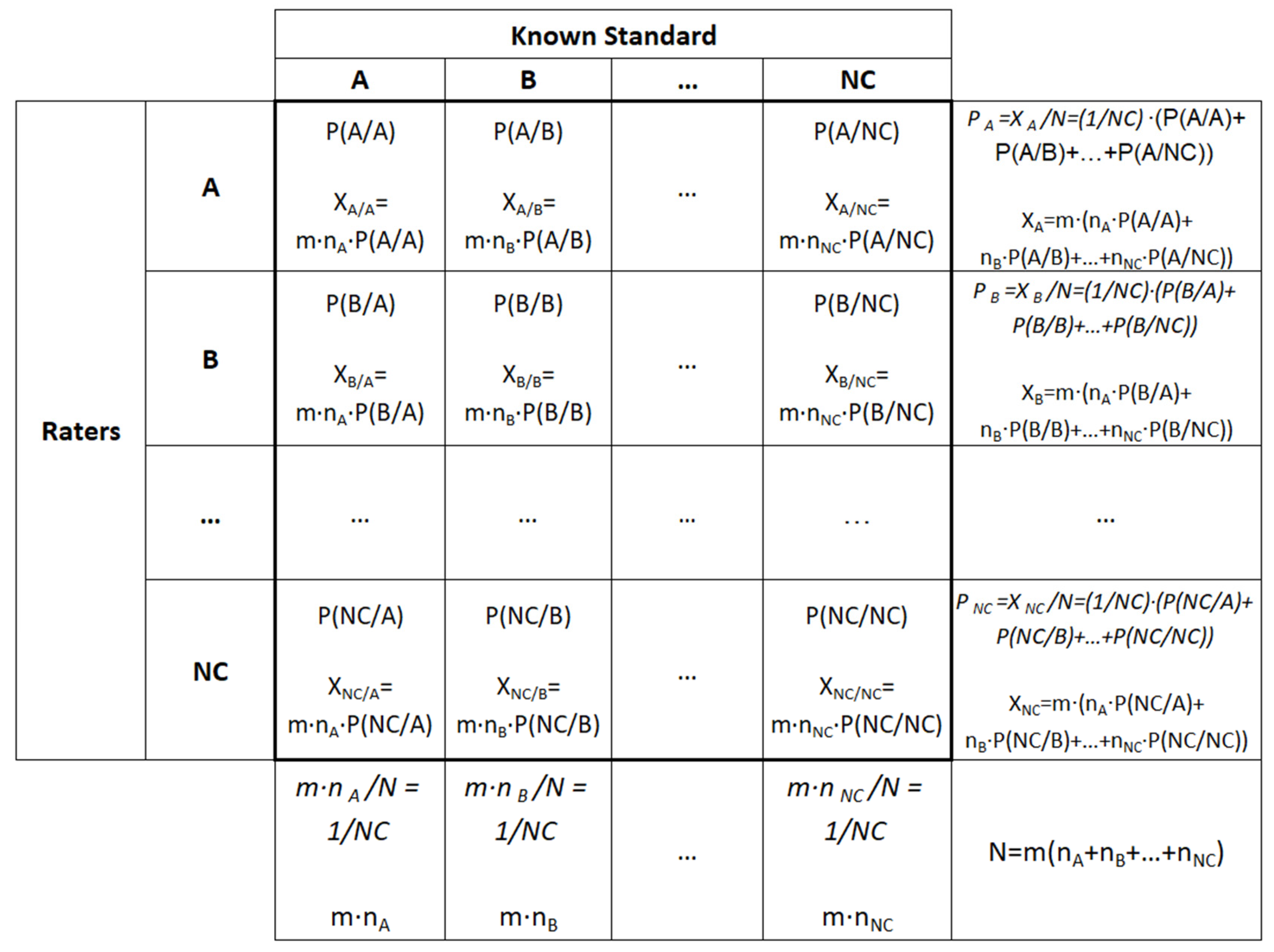
Figure 2.
Graphical representation of Eq. (4) for accuracy = 0.95: Intrinsic Kappa point estimate as a function of the number of categories.
Figure 2.
Graphical representation of Eq. (4) for accuracy = 0.95: Intrinsic Kappa point estimate as a function of the number of categories.
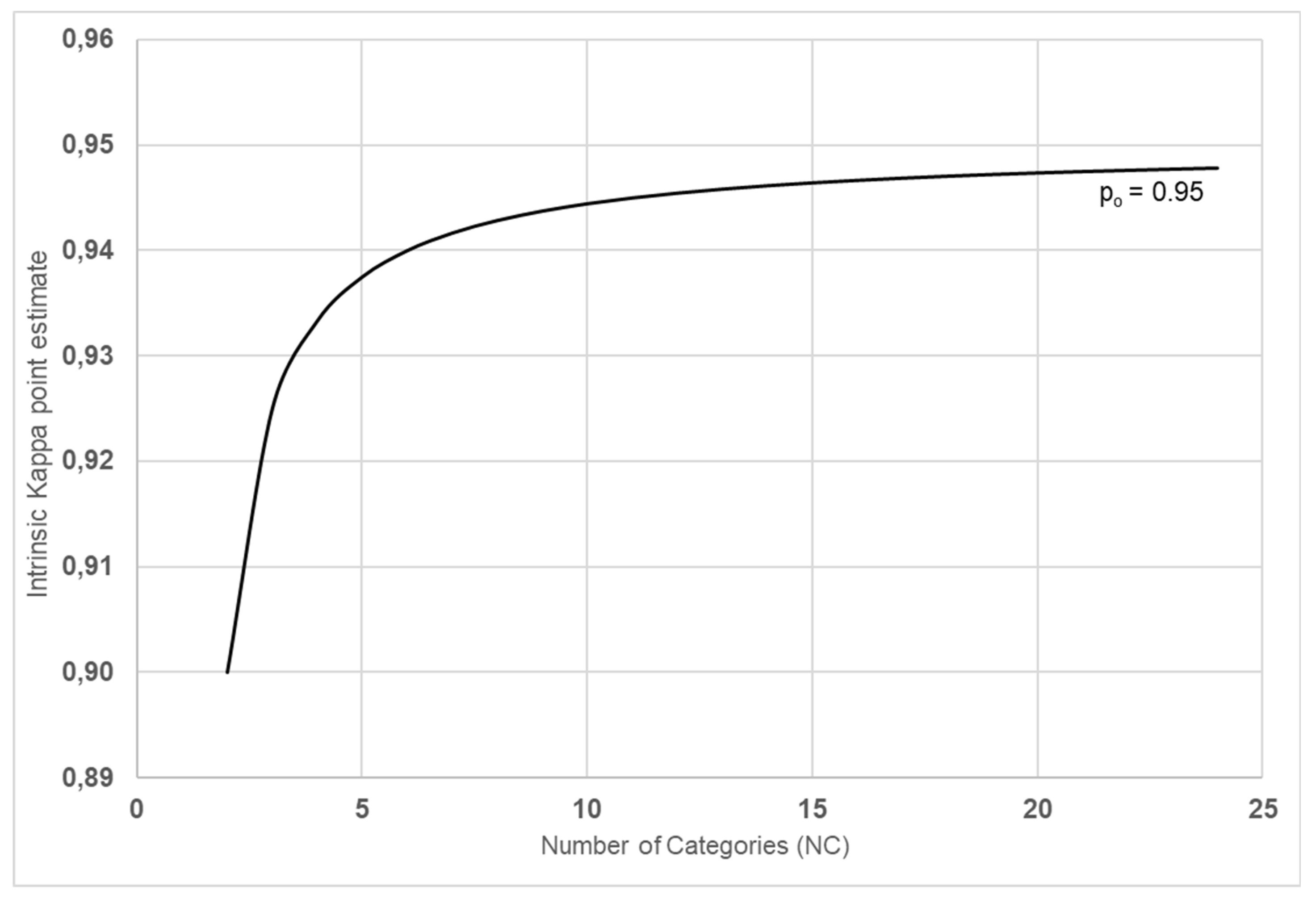

Table 1.
Intrinsic kappa lower bound. Exact vs approximate method without point-estimate adjustment for NC=2 and α = 0.05 and α = 0.05 (5%).
Table 1.
Intrinsic kappa lower bound. Exact vs approximate method without point-estimate adjustment for NC=2 and α = 0.05 and α = 0.05 (5%).
| N | Failures | Exact kLB | Approx. kLB | Rel. Error | Est. Error | |
|---|---|---|---|---|---|---|
| 100 | 5 | 0.822 | 0.9 | 0.828 | 0.81% | 7.97% |
| 100 | 25 | 0.359 | 0.5 | 0.358 | 0.35% | 28.49% |
| 200 | 5 | 0.91 | 0.95 | 0.914 | 0.44% | 3.82% |
| 200 | 50 | 0.4 | 0.5 | 0.399 | 0.09% | 20.15% |
| 500 | 5 | 0.964 | 0.98 | 0.965 | 0.19% | 1.49% |
| 500 | 50 | 0.755 | 0.8 | 0.756 | 0.16% | 5.52% |
| 500 | 100 | 0.541 | 0.6 | 0.541 | 0.07% | 9.81% |
| 1000 | 5 | 0.982 | 0.99 | 0.983 | 0.09% | 0.74% |
| 1000 | 50 | 0.876 | 0.9 | 0.877 | 0.10% | 2.52% |
| 1000 | 100 | 0.768 | 0.8 | 0.769 | 0.08% | 3.90% |
| 1000 | 250 | 0.455 | 0.5 | 0.455 | 0.00% | 9.01% |
| 2000 | 5 | 0.991 | 0.995 | 0.991 | 0.05% | 0.37% |
| 2000 | 50 | 0.938 | 0.95 | 0.939 | 0.05% | 1.21% |
| 2000 | 100 | 0.884 | 0.9 | 0.884 | 0.05% | 1.78% |
| 2000 | 250 | 0.725 | 0.75 | 0.726 | 0.04% | 3.24% |
| 2000 | 500 | 0.468 | 0.5 | 0.468 | 0.00% | 6.37% |
| 5000 | 5 | 0.996 | 0.998 | 0.997 | 0.02% | 0.15% |
| 5000 | 50 | 0.975 | 0.98 | 0.975 | 0.02% | 0.47% |
| 5000 | 100 | 0.953 | 0.96 | 0.953 | 0.02% | 0.68% |
| 5000 | 250 | 0.89 | 0.9 | 0.890 | 0.02% | 1.13% |
| 5000 | 500 | 0.786 | 0.8 | 0.786 | 0.02% | 1.74% |
| 5000 | 1500 | 0.379 | 0,4 | 0.379 | 0.01% | 5.33% |
| 50000 | 5 | 1 | 1 | 1 | 0.00% | 0.01% |
| 50000 | 50 | 0,998 | 0.998 | 0.998 | 0.00% | 0.05% |
| 50000 | 100 | 0,995 | 0.996 | 0.995 | 0.00% | 0.07% |
| 50000 | 500 | 0,979 | 0.98 | 0.979 | 0.00% | 0.15% |
| 50000 | 1000 | 0,958 | 0.96 | 0.958 | 0.00% | 0.21% |
| 50000 | 10000 | 0,594 | 0.6 | 0.594 | 0.00% | 0.98% |
| Mean Rel. Error = | 0.10% | |||||
Table 2.
Intrinsic kappa lower bound. Comparison between exact and approximate method with point estimate adjustment for NC=2 and Significance level = 0.05 (5%).
Table 2.
Intrinsic kappa lower bound. Comparison between exact and approximate method with point estimate adjustment for NC=2 and Significance level = 0.05 (5%).
| N | Failures | Exact kLB | Approx. kLB | Rel. Error | Est. Error | |
|---|---|---|---|---|---|---|
| 100 | 5 | 0.822 | 0.9 | 0.818 | 0.49% | 9.16% |
| 100 | 25 | 0.359 | 0.5 | 0.356 | 0.85% | 28.85% |
| 200 | 5 | 0.910 | 0.95 | 0.908 | 0.22% | 4.46% |
| 200 | 50 | 0.400 | 0.5 | 0.399 | 0.25% | 20.28% |
| 500 | 5 | 0.964 | 0.98 | 0.963 | 0.08% | 1.76% |
| 500 | 50 | 0.755 | 0.8 | 0.755 | 0.08% | 5.59% |
| 500 | 100 | 0.541 | 0.6 | 0.541 | 0.02% | 9.85% |
| 1000 | 5 | 0.982 | 0.99 | 0.981 | 0.04% | 0.87% |
| 1000 | 50 | 0.876 | 0.9 | 0.877 | 0.05% | 2.56% |
| 1000 | 100 | 0.768 | 0.8 | 0.769 | 0.05% | 3.93% |
| 1000 | 250 | 0.455 | 0.5 | 0.455 | 0.01% | 9.02% |
| 2000 | 5 | 0.991 | 0.995 | 0.991 | 0.02% | 0.44% |
| 2000 | 50 | 0.938 | 0.95 | 0.938 | 0.03% | 1.23% |
| 2000 | 100 | 0.884 | 0.9 | 0.884 | 0.03% | 1.80% |
| 2000 | 250 | 0.725 | 0.75 | 0.726 | 0.03% | 3.25% |
| 2000 | 500 | 0.468 | 0.5 | 0.468 | 0.00% | 6.38% |
| 5000 | 5 | 0.996 | 0.998 | 0.996 | 0.01% | 0.17% |
| 5000 | 50 | 0.975 | 0.98 | 0.975 | 0.01% | 0.48% |
| 5000 | 100 | 0.953 | 0.96 | 0.953 | 0.01% | 0.68% |
| 5000 | 250 | 0.890 | 0.9 | 0.890 | 0.02% | 1.13% |
| 5000 | 500 | 0.786 | 0.8 | 0.786 | 0.01% | 1.75% |
| 5000 | 1500 | 0.379 | 0.4 | 0.379 | 0.01% | 5.33% |
| 50000 | 5 | 1 | 1 | 1 | 0.00% | 0.02% |
| 50000 | 50 | 0.998 | 0.998 | 0.998 | 0.00% | 0.05% |
| 50000 | 100 | 0.995 | 0.996 | 0.995 | 0.00% | 0.07% |
| 50000 | 500 | 0.979 | 0.98 | 0.979 | 0.00% | 0.15% |
| 50000 | 1000 | 0.958 | 0.96 | 0.958 | 0.00% | 0.21% |
| 50000 | 10000 | 0,594 | 0.6 | 0.594 | 0.00% | 0.98% |
| Mean Rel. Error = | 0.08% | |||||
Table 3.
Intrinsic kappa lower bound. Comparison between exact and approximate method without point estimate adjustment for NC=3 and Significance level = 0.05 (5%).
Table 3.
Intrinsic kappa lower bound. Comparison between exact and approximate method without point estimate adjustment for NC=3 and Significance level = 0.05 (5%).
| N | Failures | Exact kLB | Approx. kLB | Rel. Error | Est. Error | |
|---|---|---|---|---|---|---|
| 100 | 5 | 0.866 | 0.925 | 0.871 | 0.58% | 5.81% |
| 100 | 25 | 0.519 | 0.625 | 0.518 | 0.18% | 17.10% |
| 200 | 5 | 0.932 | 0.963 | 0.935 | 0.33% | 2.83% |
| 200 | 50 | 0.550 | 0.625 | 0.549 | 0.05% | 12.09% |
| 500 | 5 | 0.973 | 0.985 | 0.974 | 0.14% | 1.11% |
| 500 | 50 | 0.816 | 0.85 | 0.817 | 0.11% | 3.89% |
| 500 | 100 | 0.656 | 0.7 | 0.656 | 0.04% | 6.31% |
| 1000 | 5 | 0.986 | 0.993 | 0.987 | 0.07% | 0.55% |
| 1000 | 50 | 0.907 | 0.925 | 0.908 | 0.07% | 1.84% |
| 1000 | 100 | 0.826 | 0.85 | 0.827 | 0.06% | 2.75% |
| 1000 | 250 | 0.591 | 0.625 | 0.591 | 0.00% | 5.41% |
| 2000 | 5 | 0.993 | 0.996 | 0.993 | 0.04% | 0.28% |
| 2000 | 50 | 0.954 | 0.963 | 0.954 | 0.04% | 0.89% |
| 2000 | 100 | 0.913 | 0.925 | 0.913 | 0.04% | 1.30% |
| 2000 | 250 | 0.794 | 0.813 | 0.794 | 0.03% | 2.25% |
| 2000 | 500 | 0.601 | 0.625 | 0.601 | 0.00% | 3.82% |
| 5000 | 5 | 0.997 | 0.999 | 0.997 | 0.01% | 0.11% |
| 5000 | 50 | 0.981 | 0.985 | 0.982 | 0.02% | 0.35% |
| 5000 | 100 | 0.965 | 0.97 | 0.965 | 0.02% | 0.50% |
| 5000 | 250 | 0.917 | 0.925 | 0.917 | 0.01% | 0.82% |
| 5000 | 500 | 0.839 | 0.85 | 0.840 | 0.01% | 1.23% |
| 5000 | 1500 | 0.534 | 0.55 | 0.534 | 0.01% | 2.91% |
| 50000 | 5 | 1 | 1 | 1 | 0.00% | 0.01% |
| 50000 | 50 | 0.998 | 0.999 | 0.998 | 0.00% | 0.03% |
| 50000 | 100 | 0.996 | 0.997 | 0.997 | 0.00% | 0.05% |
| 50000 | 500 | 0.984 | 0.985 | 0.984 | 0.00% | 0.11% |
| 50000 | 1000 | 0.968 | 0.97 | 0.968 | 0.00% | 0.16% |
| 50000 | 10000 | 0.696 | 0.7 | 0.694 | 0.21% | 0.84% |
| Mean Rel. Error = | 0.07% | |||||
Table 4.
Intrinsic kappa lower bound. Comparison between exact and approximate method with point estimate adjustment for NC=3 and Significance level = 0.05 (5%).
Table 4.
Intrinsic kappa lower bound. Comparison between exact and approximate method with point estimate adjustment for NC=3 and Significance level = 0.05 (5%).
| N | Failures | Exact kLB | Approx. kLB | Rel. Error | Est. Error | |
|---|---|---|---|---|---|---|
| 100 | 5 | 0.866 | 0.925 | 0.863 | 0.35% | 6.68% |
| 100 | 25 | 0.519 | 0.625 | 0.517 | 0.44% | 17.31% |
| 200 | 5 | 0.932 | 0.963 | 0.931 | 0.16% | 3.30% |
| 200 | 50 | 0.55 | 0.625 | 0.549 | 0.14% | 12.17% |
| 500 | 5 | 0.973 | 0.985 | 0.972 | 0.06% | 1.31% |
| 500 | 50 | 0.816 | 0.85 | 0.816 | 0.06% | 3.95% |
| 500 | 100 | 0.656 | 0.7 | 0.656 | 0.01% | 6.33% |
| 1000 | 5 | 0.986 | 0.993 | 0.986 | 0.03% | 0.65% |
| 1000 | 50 | 0.907 | 0.925 | 0.908 | 0.04% | 1.87% |
| 1000 | 100 | 0.826 | 0.850 | 0.826 | 0.04% | 2.77% |
| 1000 | 250 | 0.591 | 0.625 | 0.591 | 0.01% | 5.41% |
| 2000 | 5 | 0.993 | 0.996 | 0.993 | 0.01% | 0.33% |
| 2000 | 50 | 0.954 | 0.963 | 0.954 | 0.02% | 0.91% |
| 2000 | 100 | 0.913 | 0.925 | 0.913 | 0.02% | 1.31% |
| 2000 | 250 | 0.794 | 0.813 | 0.794 | 0.02% | 2.25% |
| 2000 | 500 | 0.601 | 0.625 | 0.601 | 0.00% | 3.83% |
| 5000 | 5 | 0.997 | 0.999 | 0.997 | 0.01% | 0.13% |
| 5000 | 50 | 0.981 | 0.985 | 0.981 | 0.01% | 0.36% |
| 5000 | 100 | 0.965 | 0.97 | 0.965 | 0.01% | 0.51% |
| 5000 | 250 | 0.917 | 0.925 | 0.917 | 0.01% | 0.82% |
| 5000 | 500 | 0.839 | 0.85 | 0.84 | 0.01% | 1.23% |
| 5000 | 1500 | 0.534 | 0.55 | 0.534 | 0.01% | 2.91% |
| 50000 | 5 | 1 | 1 | 1 | 0.00% | 0.01% |
| 50000 | 50 | 0.998 | 0.999 | 0.998 | 0.00% | 0.04% |
| 50000 | 100 | 0.996 | 0.997 | 0.997 | 0.00% | 0.05% |
| 50000 | 500 | 0.984 | 0.985 | 0.984 | 0.00% | 0.11% |
| 50000 | 1000 | 0.968 | 0.97 | 0.968 | 0.00% | 0.16% |
| 50000 | 10000 | 0.696 | 0.7 | 0.696 | 0.00% | 0.63% |
| Mean Rel. Error = | 0.05% | |||||
Table 5.
Intrinsic kappa lower bound. Comparison between exact and approximate method without point estimate adjustment for NC=10 and Significance level = 0.05 (5%).
Table 5.
Intrinsic kappa lower bound. Comparison between exact and approximate method without point estimate adjustment for NC=10 and Significance level = 0.05 (5%).
| N | Failures | Exact kLB | Approx. kLB | Rel. Error | Est. Error | |
|---|---|---|---|---|---|---|
| 100 | 5 | 0.901 | 0.944 | 0.905 | 0.41% | 4.22% |
| 100 | 25 | 0.644 | 0.722 | 0.643 | 0.11% | 10.96% |
| 200 | 5 | 0.950 | 0.972 | 0.952 | 0.24% | 2.08% |
| 200 | 50 | 0.666 | 0.722 | 0.666 | 0.03% | 7.75% |
| 500 | 5 | 0.980 | 0.989 | 0.981 | 0.10% | 0.82% |
| 500 | 50 | 0.864 | 0.889 | 0.864 | 0.08% | 2.76% |
| 500 | 100 | 0.745 | 0.778 | 0.745 | 0.03% | 4.20% |
| 1000 | 5 | 0.990 | 0.994 | 0.990 | 0.05% | 0.41% |
| 1000 | 50 | 0.931 | 0.944 | 0.932 | 0.05% | 1.33% |
| 1000 | 100 | 0.871 | 0.889 | 0.872 | 0.04% | 1.95% |
| 1000 | 250 | 0.697 | 0.722 | 0.697 | 0.00% | 3.47% |
| 2000 | 5 | 0.995 | 0.997 | 0.995 | 0.03% | 0.20% |
| 2000 | 50 | 0.966 | 0.972 | 0.966 | 0.03% | 0.66% |
| 2000 | 100 | 0.935 | 0.944 | 0.936 | 0.03% | 0.94% |
| 2000 | 250 | 0.847 | 0.861 | 0.848 | 0.02% | 1.57% |
| 2000 | 500 | 0.705 | 0.722 | 0.705 | 0.00% | 2.45% |
| 5000 | 5 | 0.998 | 0.999 | 0.998 | 0.01% | 0.08% |
| 5000 | 50 | 0.986 | 0.989 | 0.986 | 0.01% | 0.26% |
| 5000 | 100 | 0.974 | 0.978 | 0.974 | 0.01% | 0.37% |
| 5000 | 250 | 0.939 | 0.944 | 0.939 | 0.01% | 0.60% |
| 5000 | 500 | 0.881 | 0.889 | 0.881 | 0.01% | 0.87% |
| 5000 | 1500 | 0.655 | 0.667 | 0.655 | 0.00% | 1.78% |
| 50000 | 5 | 1 | 1 | 1 | 0.00% | 0.01% |
| 50000 | 50 | 0.999 | 0.999 | 0.999 | 0.00% | 0.03% |
| 50000 | 100 | 0.997 | 0.998 | 0.997 | 0.00% | 0.04% |
| 50000 | 500 | 0.988 | 0.989 | 0.988 | 0.00% | 0.08% |
| 50000 | 1000 | 0.977 | 0.978 | 0.977 | 0.00% | 0.12% |
| 50000 | 10000 | 0.775 | 0.778 | 0.775 | 0.00% | 0.42% |
| Mean Rel. Error = | 0.05% | |||||
Table 6.
Intrinsic kappa lower bound. Comparison between exact and approximate method with point estimate adjustment for NC=10 and Significance level = 0.05 (5%).
Table 6.
Intrinsic kappa lower bound. Comparison between exact and approximate method with point estimate adjustment for NC=10 and Significance level = 0.05 (5%).
| N | Failures | Exact kLB | Approx. kLB | Rel. Error | Est. Error | |
|---|---|---|---|---|---|---|
| 100 | 5 | 0.866 | 0.925 | 0.863 | 0.35% | 4.85% |
| 100 | 25 | 0.519 | 0.625 | 0.517 | 0.44% | 11.10% |
| 200 | 5 | 0.932 | 0.963 | 0.931 | 0.16% | 2.42% |
| 200 | 50 | 0.55 | 0.625 | 0.549 | 0.14% | 7.80% |
| 500 | 5 | 0.973 | 0.985 | 0.972 | 0.06% | 0.97% |
| 500 | 50 | 0.816 | 0.85 | 0.816 | 0.06% | 2.80% |
| 500 | 100 | 0.656 | 0.7 | 0.656 | 0.01% | 4.22% |
| 1000 | 5 | 0.986 | 0.993 | 0.986 | 0.03% | 0.48% |
| 1000 | 50 | 0.907 | 0.925 | 0.908 | 0.04% | 1.36% |
| 1000 | 100 | 0.826 | 0.850 | 0.826 | 0.04% | 1.96% |
| 1000 | 250 | 0.591 | 0.625 | 0.591 | 0.01% | 3.47% |
| 2000 | 5 | 0.993 | 0.996 | 0.993 | 0.01% | 0.24% |
| 2000 | 50 | 0.954 | 0.963 | 0.954 | 0.02% | 0.67% |
| 2000 | 100 | 0.913 | 0.925 | 0.913 | 0.02% | 0.95% |
| 2000 | 250 | 0.794 | 0.813 | 0.794 | 0.02% | 1.57% |
| 2000 | 500 | 0.601 | 0.625 | 0.601 | 0.00% | 2.45% |
| 5000 | 5 | 0.997 | 0.999 | 0.997 | 0.01% | 0.10% |
| 5000 | 50 | 0.981 | 0.985 | 0.981 | 0.01% | 0.27% |
| 5000 | 100 | 0.965 | 0.97 | 0.965 | 0.01% | 0.37% |
| 5000 | 250 | 0.917 | 0.925 | 0.917 | 0.01% | 0.60% |
| 5000 | 500 | 0.839 | 0.85 | 0.84 | 0.01% | 0.87% |
| 5000 | 1500 | 0.534 | 0.55 | 0.534 | 0.01% | 1.78% |
| 50000 | 5 | 1 | 1 | 1 | 0.00% | 0.01% |
| 50000 | 50 | 0.998 | 0.999 | 0.998 | 0.00% | 0.03% |
| 50000 | 100 | 0.996 | 0.997 | 0.997 | 0.00% | 0.04% |
| 50000 | 500 | 0.984 | 0.985 | 0.984 | 0.00% | 0.08% |
| 50000 | 1000 | 0.968 | 0.97 | 0.968 | 0.00% | 0.12% |
| 50000 | 10000 | 0.696 | 0.7 | 0.696 | 0.00% | 0.42% |
| Mean Rel. Error = | 0.05% | |||||
Table 7.
Accuracy lower bound. Comparison between exact and approximate method without point estimate adjustment and Significance level = 0.05 (5%).
Table 7.
Accuracy lower bound. Comparison between exact and approximate method without point estimate adjustment and Significance level = 0.05 (5%).
| N | Failures | Exact Acc.LB | Appr. Acc.LB | Rel. Error | Est. Error | |
|---|---|---|---|---|---|---|
| 100 | 5 | 0.911 | 0.95 | 0.914 | 0.37% | 3.77% |
| 100 | 25 | 0.679 | 0.75 | 0.679 | 0.09% | 9.50% |
| 200 | 5 | 0.955 | 0.975 | 0.957 | 0.21% | 1.86% |
| 200 | 50 | 0.7 | 0.75 | 0.7 | 0.03% | 6.72% |
| 500 | 5 | 0.982 | 0.99 | 0.983 | 0.09% | 0.74% |
| 500 | 50 | 0.877 | 0.9 | 0.878 | 0.07% | 2.45% |
| 500 | 100 | 0.77 | 0.8 | 0.771 | 0.02% | 3.68% |
| 1000 | 5 | 0.991 | 0.995 | 0.991 | 0.05% | 0.37% |
| 1000 | 50 | 0.938 | 0.95 | 0.939 | 0.04% | 1.19% |
| 1000 | 100 | 0.884 | 0.9 | 0.884 | 0.04% | 1.73% |
| 1000 | 250 | 0.727 | 0.75 | 0.727 | 0.00% | 3.00% |
| 2000 | 5 | 0.995 | 0.998 | 0.996 | 0.02% | 0.18% |
| 2000 | 50 | 0.969 | 0.975 | 0.969 | 0.02% | 0.59% |
| 2000 | 100 | 0.942 | 0.95 | 0.942 | 0.02% | 0.84% |
| 2000 | 250 | 0.863 | 0.875 | 0.863 | 0.02% | 1.39% |
| 2000 | 500 | 0.734 | 0.75 | 0.734 | 0.00% | 2.12% |
| 5000 | 5 | 0.998 | 0.999 | 0.998 | 0.01% | 0.07% |
| 5000 | 50 | 0.988 | 0.99 | 0.988 | 0.01% | 0.23% |
| 5000 | 100 | 0.977 | 0.98 | 0.977 | 0.01% | 0.33% |
| 5000 | 250 | 0.945 | 0.95 | 0.945 | 0.01% | 0.53% |
| 5000 | 500 | 0.893 | 0.9 | 0.893 | 0.01% | 0.78% |
| 5000 | 1500 | 0.689 | 0.7 | 0.689 | 0.00% | 1.52% |
| 50000 | 5 | 1 | 1 | 1 | 0.00% | 0.01% |
| 50000 | 50 | 0.999 | 0.999 | 0.999 | 0.00% | 0.02% |
| 50000 | 100 | 0.998 | 0.998 | 0.998 | 0.00% | 0.03% |
| 50000 | 500 | 0.989 | 0.99 | 0.989 | 0.00% | 0.07% |
| 50000 | 1000 | 0.979 | 0.98 | 0.979 | 0.00% | 0.11% |
| 50000 | 10000 | 0.797 | 0.80 | 0.797 | 0.00% | 0.37% |
| Mean Rel. Error = | 0.04% | |||||
Table 8.
Accuracy lower bound. Comparison between exact and approximate method with point estimate adjustment and Significance level = 0.05 (5%).
Table 8.
Accuracy lower bound. Comparison between exact and approximate method with point estimate adjustment and Significance level = 0.05 (5%).
| N | Failures | Exact Acc.LB | Appr. Acc. LB | Rel. Error | Est. Error | |
|---|---|---|---|---|---|---|
| 100 | 5 | 0.911 | 0.95 | 0.909 | 0.22% | 4.34% |
| 100 | 25 | 0.679 | 0.75 | 0.678 | 0.22% | 9.62% |
| 200 | 5 | 0.955 | 0.975 | 0954 | 0.10% | 2.17% |
| 200 | 50 | 0.7 | 0.75 | 0.699 | 0.07% | 6.76% |
| 500 | 5 | 0.982 | 0.99 | 0.981 | 0.04% | 0.87% |
| 500 | 50 | 0.877 | 0.9 | 0.878 | 0.03% | 2.49% |
| 500 | 100 | 0.77 | 0.8 | 0.77 | 0.01% | 3.69% |
| 1000 | 5 | 0.991 | 0.995 | 0.991 | 0.02% | 0.44% |
| 1000 | 50 | 0.938 | 0.95 | 0.938 | 0.02% | 1.21% |
| 1000 | 100 | 0.884 | 0.9 | 0.884 | 0.02% | 1.75% |
| 1000 | 250 | 0.727 | 0.75 | 0.727 | 0.00% | 3.01% |
| 2000 | 5 | 0.995 | 0998 | 0.995 | 0.01% | 0.22% |
| 2000 | 50 | 0.969 | 0.975 | 0.969 | 0.01% | 0.60% |
| 2000 | 100 | 0.942 | 0.95 | 0.942 | 0.02% | 0.85% |
| 2000 | 250 | 0.863 | 0.875 | 0.863 | 0.01% | 1.39% |
| 2000 | 500 | 0.734 | 0.75 | 0.734 | 0.00% | 2.13% |
| 5000 | 5 | 0.998 | 0.999 | 0.998 | 0.00% | 0.09% |
| 5000 | 50 | 0.988 | 0.99 | 0.988 | 0.01% | 0.24% |
| 5000 | 100 | 0.977 | 098 | 0.977 | 0.01% | 0.34% |
| 5000 | 250 | 0.945 | 0.95 | 0.945 | 0.01% | 0.54% |
| 5000 | 500 | 0.893 | 0.9 | 0.893 | 0.01% | 0.78% |
| 5000 | 1500 | 0.689 | 0.7 | 0.689 | 0.00% | 1.52% |
| 50000 | 5 | 1 | 1 | 1 | 0.00% | 0.01% |
| 50000 | 50 | 0.999 | 0.999 | 0.999 | 0.00% | 0.02% |
| 50000 | 100 | 0.998 | 0.998 | 0.998 | 0.00% | 0.03% |
| 50000 | 500 | 0.989 | 0.99 | 0.989 | 0.00% | 0.07% |
| 50000 | 1000 | 0.979 | 0.98 | 0.979 | 0.00% | 0.11% |
| 50000 | 10000 | 0.797 | 0.8 | 0.797 | 0.00% | 0.37% |
| Mean Rel. Error = | 0.03% | |||||
Disclaimer/Publisher’s Note: The statements, opinions and data contained in all publications are solely those of the individual author(s) and contributor(s) and not of MDPI and/or the editor(s). MDPI and/or the editor(s) disclaim responsibility for any injury to people or property resulting from any ideas, methods, instructions or products referred to in the content. |
© 2025 by the authors. Licensee MDPI, Basel, Switzerland. This article is an open access article distributed under the terms and conditions of the Creative Commons Attribution (CC BY) license (http://creativecommons.org/licenses/by/4.0/).
Copyright: This open access article is published under a Creative Commons CC BY 4.0 license, which permit the free download, distribution, and reuse, provided that the author and preprint are cited in any reuse.


