
Submitted:
29 May 2025
Posted:
01 June 2025
You are already at the latest version
Abstract
Fiber-reinforced composite materials exhibit orthotropic behavior, characterized by complex orthotropic engineering constants such as Young’s modulus, Poisson’s ratio, and shear modulus. It is widely recognized that basalt fibers possess superior resistance to elevated temperatures compared to glass fibers. However, the behavior of these fibers within composites at typical operational temperatures for automotive and consumer goods applications has not been thoroughly investigated. A novel measurement setup based on the non-destructive impulse excitation method has been developed for the automated identification of the complex orthotropic engineering constants as a function of temper-ature. This study provides a comparative analysis of the identified engineering constants of bidirectionally fabric-reinforced glass and basalt composites with an epoxy matrix, across a temperature range from -20 °C to 60 °C. The results reveal only minimal dif-ferences in stiffness and damping behavior between the examined glass and basalt samples.
Keywords:
Temperature dependency
; Complex Engineering constants
; Glass fiber
; Basalt fiber
; Composites
1. Introduction
1.1. Glass Fibre-Reinforced Polymer (GFRP) Composites
GFRP composites have gained widespread adoption across various industries due to their excellent properties, including high tensile strength, flexibility, and chemical resistance, see e.g. [1]. These composites can be fabricated using a range of manufacturing technologies and are employed in numerous applications. The reinforcing glass fibers (GF) are available in forms such as rovings, chopped strands, yarns, fabrics, and mats. Thermoset GFRP composites are produced through processes such as, among others, compression molding, hot press molding, resin transfer molding, reaction injection molding, and vacuum-assisted molding. In contrast, thermoplastic composites are manufactured using plunger and screw-type injection molding machines. The versatility of GFRP composites extends to their use in the automotive, aerospace, and construction sectors, where their low density and high strength provide significant advantages, see e.g. [2,3].
1.2. Basalt Fiber-Reinforced Polymer (BFRP) Composites
Basalt fibers (BF) represent a relatively new material with potential to replace glass fibers in composite materials. The production process involves melting basalt rock at high temperatures, resulting in relatively low environmental impact compared to synthetic polymers, see e.g. [4,5]. Filament diameters ranging from 7 microns to 17 microns can be produced, depending on the fiber drawing speed and melting temperature. Like GF, BF can be manufactured in forms such as rovings, chopped strands, yarns, fabrics, and mats. The elastic modulus of BF, which depends on its chemical composition, is typically equal to or somewhat superior to that of GF, see e.g. [6]. Some studies indicate that BF offers superior mechanical strength compared to GF, see e.g. [7]. However, the stiffness and damping behavior of BF-reinforced composites at typical operational temperatures for automotive and consumer goods applications have not been thoroughly investigated or compared with similar GF-reinforced composites.
1.3. Elastic and Damping Properties of Composite Materials
The elastic properties of composite material parts are critical in determining their deformation under static and dynamic loads. The vibration and acoustic behavior of these materials are influenced by their elastic and damping properties. Temperature variations change the elastic and damping characteristics of composite materials, leading to alternations in resonance frequencies, mode shapes, and transient responses, which can impact the functional performance of vehicles, construction components, and consumer goods. Therefore, understanding the temperature-dependent elastic and damping properties is essential for a reliable design of composite structures.
The elastic and damping behavior of a material in a thin sheet with linear material properties can be described by engineering constants: Young's modulus (E), Poisson's ratio (v), and in-plane shear modulus (G). In a statically loaded sheet, normal stresses and shear stresses occur, resulting in both normal and shear strains. Young's modulus (E) in a material point is the ratio of normal stress to normal strain (see Figure 1a). Poisson's ratio (v) is the negative ratio of normal strain in one direction to normal strain in the perpendicular direction (see Figure 1b). The in-plane shear modulus (G) is the ratio of shear stress to shear strain (see Figure 1c).
When the sheet is dynamically loaded with a sinusoidal load at a circular frequency (ω), the dynamic Young's modulus (E(ω)) is the ratio of stress amplitude to strain amplitude (see Figure 2). Similarly, the dynamic Poisson's ratio (v(ω)) and the dynamic in-plane shear modulus (G(ω)) are the ratios of amplitudes. Damping can cause a phase shift between the sinusoidal stress and strain signals (see Figure 2). This is the case for viscoelastic materials like polymers and polymer composites. The value of the dynamic engineering constants can vary as a function of the circular frequency (see e.g. [8]).
For isotropic materials, the elastic properties are the same in each direction. Most composites, however, exhibit orthotropic behavior. Orthotropic materials have elastic properties symmetric with respect to a Cartesian coordinate system. Five engineering constants are required to describe the orthotropic in-plane elastic behavior of thin sheets. In a plane with two perpendicular orthotropic material directions 1 and 2 (see Figure 3), the five engineering constants are E1 (Young’s modulus in the 1-direction), E2 (Young’s modulus in the 2-direction), v12 (Major Poisson’s ratio with major strain in the 1-direction and contraction strain in the 2-direction), v21 (Minor Poisson’s ratio with minor strain in the 2-direction and contraction strain in the 1-direction), and G12 (In-plane shear modulus in the (1,2) plane).
The relation between stresses and strains in an orthotropic composite sheet is given by the stiffness matrix [C], see e.g. [9]:
In the case of pure elastic behavior, the engineering constants have only real values. In the case of viscoelastic behavior, the quantities in (1) are all complex numbers with real and imaginary parts. [C*] is the complex in-plane stiffness matrix, , are normal strains and ,are normal stresses, respectively in the 1- and 2-direction. , are the in-plane shear strains and stresses.
, are the complex dynamic Young’s moduli, , are the major and minor Poisson’s ratios and is the complex in-plane shear modulus. For a given circular frequency and assumed linear behavior, the values are constant and called the complex dynamic Engineering constants. Because of the symmetry of the stiffness matrix [C*], and therefore there are only 4 independent complex Engineering constants in C*. These are shown in equations (2)
The real parts in the equation (2) represent the elastic behavior while the imaginary “tangents delta” parts govern the damping contribution in the complex Engineering constants.
1.4. A Novel Setup to Measure Orthotropic Engineering Constants
A novel measurement setup utilizing a non-destructive impulse excitation method has been developed for the automated identification of complex orthotropic engineering constants as a function of temperature. In this study, the measurement setup is employed to provide a comparative analysis of the identified engineering constants of glass and basalt bidirectionally fabric-reinforced composites with an epoxy matrix, across a temperature range from -20 °C to 60 °C. The first chapter of this article will describe briefly static standard methods, standard dynamic methods and the new measurement setup. Subsequently, the tested materials and measurement results will be discussed.
2. Measurement of Engineering Constants of Composite Materials
Various test methods exist for measuring engineering constants, categorized into static and dynamic measurement methods.
2.1. Static Measurement Methods
Well-known static methods include tensile testing, bending, shear, and torsion tests. Engineering constants are determined based on measured forces, longitudinal and transverse deformations (see, e.g. [10]). Flexural testing in three or four-point bending is an alternative to tensile testing, applying much smaller forces and achieving larger displacements. Calculations are typically based on thin-beam flexure equations, as described in ASTM D7264/D7264M-21 [11]. Experimental results always come with a level of uncertainty. Factors affecting uncertainty in static testing are discussed in Kostic [12]. The most influential source of uncertainty in determining the engineering constants of composite materials via static testing is the test system (dimensional measurement device, gauge determination system, extensometer type, alignment system, test machine stiffness, force measurement accuracy, extensometer accuracy), as noted by Lord and Morrell [13]. Due to inevitable imperfections in the sensors, force and displacement measurements at low stress and strain values near the origin of the stress-strain curve have high relative uncertainty bounds.
2.2. Dynamic Measurement Methods
Dynamic testing methods are indirect. The impulse excitation technique (IET) (see, e.g. [14]) and dynamic mechanical analysis (DMA) (see, e.g. [15]) are the most used dynamic methods. Dynamic testing methods are more challenging to understand intuitively but are easier to execute and provide more accurate engineering constants at low stress and strain amplitudes, as noted by Lord and Morrell [13]. The DMA uses forced excitation to measure the elastic and damping properties of composite beams within a limited frequency range, allowing the identification of temperature and frequency-dependent elastic and damping properties. Unfortunately, most DMA equipment can only handle small beam samples, which is a disadvantage for testing composite materials [16]. IET can be easily applied to large beam samples, is easy to perform, and does not require complex equipment. Simply tapping the test sample causes a low-amplitude vibration response that can be measured with a sensor and is called the "impulse response function" (IRF). The IRF comprises decaying excited modes of vibration of the test sample. The resonance frequencies and damping ratios can be extracted from the measured IRF, Heritage [17]. Because IET is non-destructive, it is suitable for testing at different temperatures, Brebels [18]. Because of all these advantages, IET was selected for the current study. The standard IET uses analytical and empirical formulas to derive the elastic properties from the measured vibration quantities. Unfortunately, no formulas are available for freely suspended orthotropic plates. To solve this problem, Sol [19] demonstrated in 1986 the possibility of replacing standard IET formulas with special-purpose finite-element (FE) models. He used a mixed numerical-experimental technique (MNET) to identify orthotropic engineering constants. The resulting identification method, called the 'Resonalyser' procedure, can simultaneously identify the four engineering constants of an orthotropic material from resonance frequencies of two test beams and a test plate measured by IET. The Resonalyser procedure is a multi-sample IET that extracts the resonance frequencies and damping ratios from the IRF’s measured on a thin orthotropic rectangular test plate and two test beams. The test beams were cut along two in-plane orthotropic directions (Figure 4). The length to width aspect ratio L/W of the test plate was adjusted according to the following formula (3):
The resonance frequencies f1 and f2 were associated with the fundamental bending vibration modes of the two test beams. L1 and L2 are the lengths of the beams. The aspect ratio L/W creates the so-called “Poisson” plate. The first five resonance frequencies of a Poisson plate are always associated with the torsion, saddle, breathing and two combinations of torsion and bending vibration modes (see Figure 5).
The orthotropic engineering constants are parameters in the numerical models of the beams and plate. These were iteratively tuned to match the computed resonance frequencies with the measured frequencies. Because the vibration modes of the first five resonance frequencies are known, no full modal analysis is necessary to identify the type of vibration mode sequence. An interesting property of a Poisson plate is that the saddle and breathing vibration modes are highly sensitive to variations in Poisson’s ratio, as shown by Lauwagie [20]. Knowledge of the type of vibration mode, together with the three first measured resonance frequencies, allows the generation of good starting values for the engineering constants G12 and v12 using the virtual field method, Pierron [21]. A detailed mathematical derivation can be found in a study by Sol et al. [22]. Validation of the results obtained using the Resonalyser procedure has been presented in several publications [23,24,25]. In 1995, De Visscher [26] extended the Resonalyser procedure to identify the damping part of the complex orthotropic engineering constants. Detailed information on how the damping part can be computed from the measured FRF can be found in [26]. Information and examples of the extended Resonalyser method can be found in [27].
Over the past few decades, various authors have presented MNET approaches for identifying orthotropic elastic constants [28,29,30,31,32,33,34,35,36,37,38,39,40,41,42,43,44]. Most methods require the measurement of modal shapes associated with resonance frequencies by using experimental modal analysis techniques. Modal analysis allows measurement on large composite material plate samples but is more difficult to execute as a function of temperature than IET. Therefore, the extended Resonalyser procedure was selected for continuous identification of engineering constants across different temperatures in a climate chamber. At different temperature steps across a desired temperature range, the IRF of the test beams and Poisson plate were obtained with an automated excitation system. This allowed the identification of the orthotropic engineering constants at each temperature step. Automated excitation uses pendulum impact activated by solenoids. The pendulum was connected through a small aperture in the climate chamber wall (Figure 6).
The pendulum mechanism is actuated using a solenoid (yellow in Figure 6a). Upon activation by a voltage, the solenoid propels a lever (dark blue in Figure 6), which strikes the wall of the climate chamber. Owing to inertia, the pendulum was set in motion until it impacted on the sample (red star in Figure 6b). The sample received an impulse and oscillated, while the pendulum mass rebounded. Gravity pulls the lever back to its initial position (Figure 6c). All components of the pendulum mechanism returned to their starting positions, while the sample continued to oscillate (Figure 6c). Three pendulum systems simultaneously excited the two beams and the plate sample in the climate chamber.
It is essential that the temperature distribution within the sample remain homogeneous across all temperature steps. The transient heat conduction in a thin sheet is influenced by convection occurring at the surfaces. The temperature profile of the samples varies over time at different internal positions, with the surface temperature changing relatively quickly, whereas the temperature at the midplane changes more slowly. Key control parameters include the convection heat-transfer coefficient h, thermal conductivity k, specific heat capacity Cp, and density ρ of the composite material of the sample [45]. Further details on the automated excitation and temperature distribution in the test samples can be found in [28].
A description of the tested materials and graphical representation of the test results are provided in the next paragraph. At the end of this paper, a comparison of the elastic and damping behavior between GFRP and BFRP in a temperature range of -20 °C to 60 °C is provided.
3. Tested Materials
The aim of this study was to compare two similar samples, the only difference being the type of fiber reinforcement. The first sample, a bidirectional glass G300 fabric reinforced composite sample GFRP had an MTB350 enhanced epoxy matrix and was composed of eight layers with a weave pattern known as "8-Harness Satin” (8HS). The fiber volume fraction was 47 %. The sample thickness was 2 mm, and the density was 1874 kg/m3. Figure 7 (left) shows a patch of the 8HS glass fabric.
The second sample, a bidirectional basalt TT320 fabric-reinforced composite sample BFRP had an MTB350 enhanced epoxy matrix and was composed of eight layers with a 7HS weave pattern. The fiber volume fraction was 45 %. The sample thickness was 2.17 mm, and the density was 1876 kg/m3. Figure 7 (right) shows a patch of basalt 7HS fabric.
The warp direction for both samples in Figure 7 is referred as the 1-direction or 0° direction. The weft direction is referred to as the 2-direction or 90° direction. A 7HS weave pattern is only slightly stiffer in the weft direction than an 8HS weave pattern.
The sizes and masses of the tested beams and plates are presented in Table 1.
4. Measurement of the Young’s Modulus by 3-Point Bending and IET
The standard EIT was executed continuously across a temperature range of -20 °C to 60 °C on the same test samples in an ARS 0390 climate chamber manufactured by ESPEC CORP. Contrary to static testing, IET directly provides Young’s modulus at very low displacement and force values using the formula provided in ASTM C 1259–98 [14]:
In equation (4), f is the frequency measured on a free-free test beam, L is the length of the beam, M is the mass, b is the width and t is the thickness.
The three-point bending test was conducted using a universal testing machine, Tinius Olsen 5 ST, across a temperature range of -20 °C to 60 °C, with increments of 10 °C. The test bench was housed in a temperature chamber (TH2700) manufactured by Grip Engineering GmbH. The cooling was facilitated by liquid nitrogen, which was controlled by a magnet valve located at the back of the chamber. The instrument was equipped with a 2.5 kN load cell, and measurements were taken with a span of 8 cm and a displacement speed of 1 mm/min. The accuracy of the load cell and displacement was 1%. The Young’s modulus of 3-point bending test could not be computed directly from the force and displacement near the origin because of the uncertainty of the force and displacement values at very low values. Therefore, the Young’s modulus of the samples was calculated using linear regression between a force of 100 Newton and zero. Figure 8 shows an example of a recorded force-displacement curve, where the red line in the figure is the regression line.
The measurement procedure and formula for the computation of Young’s modulus are given in ASTM D7264/D7264M-21 [11]:
In equation 5, F = 100 Newton applied in the middle of the span, L = 0.08 m is the length of the span between the supports, u is the displacement measured by curve fitting between zero and 100 Newton, b is the width, and t is the thickness.

Table 2.
Test results for Young’s modulus of GFRP.
| Young’s modulus E1 (0°) [GPa] |
Young’s modulus E2 (90°) [GPa] |
|||
|---|---|---|---|---|
| Temperature [°C] | 3-point bending | IET | 3-point bending | IET |
| -20 | 26.6 | 27.8 | 23.6 | 25.7 |
| -10 | 26.3 | 27.6 | 24.2 | 25.5 |
| 0 | 26.0 | 27.4 | 24.0 | 25.4 |
| 10 | 26.8 | 27.2 | 24.0 | 25.2 |
| 20 | 25.5 | 27.1 | 23.7 | 25.0 |
| 30 | 25.6 | 26.9 | 23.4 | 24.8 |
| 40 | 24.7 | 26.7 | 22.5 | 24.6 |
| 50 | 24.3 | 26.5 | 21.9 | 24.4 |
| 60 | 24.0 | 26.2 | 21.6 | 24.0 |
Table 3.
Test results for Young’s modulus of BFRP.
| Young’s modulus E1 (0°) [GPa] |
Young’s modulus E2 (90°) [GPa] |
|||
|---|---|---|---|---|
| Temperature [°C] | 3-point bending | IET | 3-point bending | IET |
| -20 | 25.1 | 26.1 | 23.3 | 25.8 |
| -10 | 23.6 | 26.0 | 23.6 | 25.6 |
| 0 | 24.0 | 25.8 | 24.3 | 25.5 |
| 10 | 23.9 | 25.6 | 23.2 | 25.3 |
| 20 | 23.9 | 25.4 | 22.9 | 25.1 |
| 30 | 24.2 | 25.3 | 22.4 | 24.8 |
| 40 | 22.6 | 25.0 | 22.2 | 24.7 |
| 50 | 22.2 | 24.8 | 21.9 | 24.5 |
| 60 | 21.9 | 24.4 | 21.4 | 24.0 |
Figure 9 shows the Young’s modulus (in Gpa) for both BFRP and GFRP (3-point bending and standard IET results) as a function of the temperature. It can be observed that the difference between the Young’s moduli E1 and E2 of GFRP and BFRP was very small. It can also be seen that the static 3-point bending results are systematically slightly lower than the values from the dynamic IET tests. This can be easily explained by the viscoelastic nature of fiber-reinforced polymers.
5. Automated Testing with the Extended Resonalyser Procedure
5.1. Measurement Results (Frequency and Damping Ratio Plots)
Figure 10 and Figure 11 show the results obtained by using automated IET testing equipment. The resonance frequencies associated with the fundamental bending modal shapes of Beam 1 (Figure 10a) and Beam 2 (Figure 10b), the resonance frequency associated with the torsional modal shape (Figure 10c), and the resonance frequencies associated with the breathing modal shape (Figure 10d) of both the GFRP and BFRP samples are shown in Figure 10. The resonance frequencies of the basalt-reinforced samples (brown in Figure 10) are slightly higher than those of the glass-reinforced samples (blue in Figure 10). All measured frequencies decreased monotonously with increasing temperature. Figure 11 shows the measured damping ratios of the test beams and Poisson plate. It can be observed in Figure 11 that the damping curves (thin blue and brown lines) show more noise than the measured frequencies in Figure 10. The damping curves were therefore smoothed with polynomials (thick blue and brown lines) before their values were used for identification of the damping part of the engineering constants (see Figure 13).
The damping ratios associated with the fundamental bending modal shapes of Beam 1 (Figure 11a) and Beam 2 (Figure 11b), the damping ratio associated with the torsional modal shape (Figure 11c), and the damping ratios associated with the breathing modal shape (Figure 11d) of both the GFRP and BFRP samples are shown in Figure 11.
5.2. Identified Engineering Constants (Moduli and Tangents Delta)
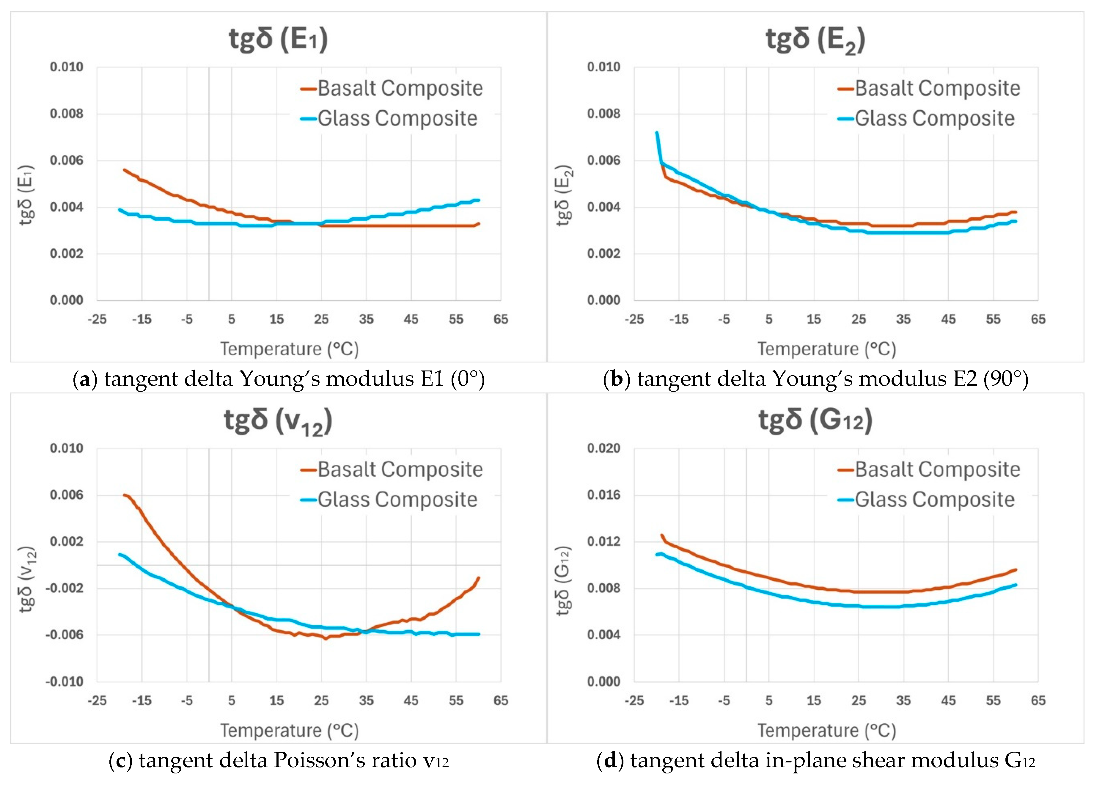
At each temperature step, the measured resonance frequencies and damping ratios were used in the Resonalyser procedure to identify the real (elastic) part and tangent delta (damping) part of the orthotropic engineering constants of the GFRP and BFRP samples between -20 °C and 60 °C. The results are shown in Figure 12 (real part) and Figure 13 (tangents delta). It can be observed in Figure 12a that the values of Young’s modulus E1 in the warp direction of GFRP are slightly bigger than those of BFRP for the whole considered temperature range. The values of the Young’s modulus in the weft direction E2 of GFRP (Figure 12b) are equal to those of BFRP for all temperatures: both curves coincide.
The same observation of coincidence is valid for both curves of Poisson’s ratio in Figure 12c. The shear modulus curves have the same evolution as the Young’s modulus in the warp direction, the G12 values of the GFRP curve are slightly bigger than those of BFRP for the whole considered temperature range. Finally, it can be remarked that all the curves of Figure 12 have decreasing values from -20 °C towards 60 °C.
The curves for the tangent delta in Figure 13 are nearly coinciding but are not monotonously decreasing like the real parts of the engineering constants. The curves show minimal values around room temperature and then increase with increasing temperature.
Figure 13.
Tangents delta of the engineering constants of GFRP and BFRP samples.
6. Discussion
The temperature interval from -20 °C to 60 °C was selected for its relevance to many vehicles and consumer goods. Generally, the observation is that the differences of the engineering constants between the GFRP and BFRP are minimal in this studied temperature interval. Some details, however, require some discussion. In Figure 10, all the frequency values of the BFRP beam samples are bigger than those of the GFRP, while in Figure 12 the Young’s modules of the GFRP beams appear to be bigger than those of the BFRP beams. This can be explained by the bigger thickness value of the BFRP beams (about 2.2 mm) as compared to the thickness of the GFRP beams (about 2 mm). The resonance frequencies of beams increase linearly with thickness t, as can be seen by rewriting formula (4) into formula (6):
The measured damping ratios as a function of temperature in the plots of Figure 11 show more noise than the plots of measured frequencies in Figure 10. The explanation for this observation is that damping is principally governed by the matrix of the composites. The temperature distribution in the matrix at subsequent temperature steps can never be 100 % homogeneous in all positions in the samples. The temperature heterogeneities cause variations in the damping value. The measured frequencies are principally governed by the stiffness of the fiber reinforcements which are less influenced by small temperature fluctuations.
The increase of the delta tangent values towards 60°C is very small. This is an indication that 60°C is still far from the glass transition temperature of the matrix material.
7. Conclusions
The IET was selected for the described study because of the many advantages as a dynamic method. It is nondestructive, accurate and easy to automate. The proposed automated resonalyser procedure uses simultaneously IET on two beams and a Poisson plate and allows identification of complex orthotropic engineering constants as a function of temperature. No experimental modal analysis was required. The resulting engineering constants are identified at low strains and stresses and hence are suitable for usage in linear analysis of deformations of construction parts. Engineering constants are mechanical parameters, necessary for linear deformation analysis, acoustic and vibration studies. In the presented study, no major differences between the engineering constants of glass and basalt reinforced composites in the considered temperature interval of -20 °C to 60 °C could be found. For applications in which the strength of the materials is important, only a study with appropriate static methods in the same temperature range can give answers.
Author Contributions
Conceptualization, H.R.; methodology, H.S.; software, H.S.; validation, J.G., G.N. and G.M.H.; investigation, J.G., G.N. and G.M.H.; resources, J.G.; writing—original draft preparation, H.S.; writing—review and editing, H.R.; visualization, J.G., G.N. and G.M.H.; supervision, H.R.; project administration, H.R. All authors have read and agreed to the published version of the manuscript.
Data Availability Statement
Material information available in the article
Conflicts of Interest
The authors declare no conflicts of interest
Abbreviations
The following abbreviations are used in this manuscript:
| IET | Impulse excitation technique |
| IRF | Impulse response function |
| DMA | Dynamic mechanical analysis |
| FE | Finite element |
| ASTM | American Standard Testing Materials |
| GF | Glass fiber |
| BF | Basalt fiber |
| GFRP | Glass fiber reinforced plastic |
| BFRP | Basalt fiber reinforced plastic |
References
- Sathishkumar T P, Satheeshkumar S , Naveen Jesuarockiam; Glass fiber-reinforced polymer composites – a review, June 2014, Journal of Reinforced Plastics and Composites 33(13):1258-1275. [CrossRef]
- Jashanpreet Singh, Kumar Satish, Saroj Kumar Mohapatra, Mandeep Kumar; Properties of Glass Fiber Hybrid Composites: A Review January 2017, Polymer-Plastics Technology and Engineering 56(5):455–469. [CrossRef]
- Muqsit Minhaj Pirzada; Recent Trends and Modifications in Glass Fibre Composites – A Review, International Journal of Materials and Chemistry 2015, 5(5): 117-122.
- Hafsa Jamshaid, Rajesh Mishra; A green material from rock: basalt fiber – a review, The Journal of The Textile Institute, Volume 107, 2016 - Issue 7. [CrossRef]
- Sami Sbahieh, Sami G. Al-Ghamdi, Gordon Mckay; A comparative life cycle assessment of fiber-reinforced polymers as a sustainable reinforcement option in concrete beamsFront. Built Environ., 22 May 2023, Sec. Sustainable Design and Construction, Volume 9 - 2023. [CrossRef]
- Mauro Henrique Lapena, Gerson Marinucci; Mechanical Characterization of Basalt and Glass Fiber Epoxy Composite Tube Materials Research. 2018; 21(1): e20170324. [CrossRef]
- Ashokkumar R. Tavadi, Yuvaraja Naik, K. Kumaresan, N.I. Jamadar, C. Rajaravi; Basalt fiber and its composite manufacturing and applications: An overview International Journal of Engineering, Science and Technology, Vol. 13, No. 4, 2021, pp. 50-56 Ashokkumar. [CrossRef]
- R.M. Christensen, Theory of viscoelasticity, an introduction, Academic Press, 1971 .
- Hashin, Z., Complex moduli of viscoelastic composites: general theory and application to particulate composites, Int. J. Solids Structures, Pergamon Press 1970, Volume 6, pp. 539 to 552. Hasshin. [CrossRef]
- ASTM D3039; Standard test method for tensile properties of polymer matrix composite materials. ASTM.
- ASTM D7264/D7264M-21; Standard Test Method for Flexural Properties of Polymer Matrix Composite Materials ASTM.
- Sonja Kostic, Jasmina Miljojkovic, Goran Simunovic, Djordje Vukelic, Branko Tadic; Uncertainty in the determination of elastic modulus by tensile testing, Engineering Science and Technology, an International Journal 25 (2022).Kostic. [CrossRef]
- J.D. Lord, R.M. Morrell; Elastic Modulus Measurement, Good Practice Guide No.98, National Physical Laboratory, 2006, Elastic modulus measurement. | NPL Publications.Lord.
- ASTM C 1259–98; Standard test methods for dynamic Young’s modulus, shear modulus and Poisson’s ratio for advanced ceramics by impulse excitation of vibration.ASTM.
- Schalnat, J. et al. Influencing parameters on measurement accuracy in dynamic mechanical analysis of thermoplastic polymers and their composites. Polymer testing 91, 106799 (2020).Schalnat. [CrossRef]
- Ashok, R.B., Srinivasa, C.V. & Basavaraju, B. Dynamic mechanical properties of natural fiber composites—a review. Adv Compos Hybrid Mater 2, 586–607 (2019). [CrossRef]
- Heritage, K.; Frisby, C.; Wolfenden, A.; Impulse excitation technique for dynamic flexural 740 measurements at moderate temperature, Review of Scientific Instruments 1988, Volume 59, pp. 973.Heritage. [CrossRef]
- Brebels Adriaan, Bollen Bart; Non-Destructive Evaluation of Material Properties as Function of Temperature by the Impulse Excitation Technique, Vol.20 No.6 (June 2015) - The e-Journal of Non-destructive Testing - ISSN 1435-4934. Brebels.
- Sol H.; Identification of anisotropic plate rigidities using free vibration data, PhD. Thesis, Vrije Universiteit Brussel, October 1986.Sol.
- T. Lauwagie, K. Lambrinou, H. Sol, W. Heylen; Resonant-Based Identification of the Poisson’s Ratio of Orthotropic Materials, Experimental Mechanics, Volume 50, pp. 437–447, (2010). Lauwagie. [CrossRef]
- Pierron, F., Grediac, M.; The virtual fields method, Springer 2012, ISBN 978 1 7614 1825 8. Pierron.
- Hugo Sol, Hubert Rahier, Jun Gu; Prediction and Measurement of the Damping Ratios of Laminated Polymer Composite Plates, MDPI, Materials (Basel), Materials, Volume 13, Issue 152020, 2020. Sol. [CrossRef]
- De Baer, I; Experimental and Numerical Study of Different Setups for Conducting and Monitoring Fatigue Experiments of Fibre-Reinforced Thermoplastics, PhD thesis University Ghent, Belgium, 2008. DeBaer.
- T. Lauwagie, H. Sol, W. Heylen; Handling uncertainties in mixed numerical-experimental techniques for vibration-based material identification, Journal of Sound and Vibration 291 (2006) pp. 723–739.Lauwagie. [CrossRef]
- Lauwagie T., Sol H., Roebben G., Heylen W., Shi Y.; Validation of the Resonalyser method: an inverse method for material identification, Proceedings of ISMA 2002, International Conference on 734 Noise and Vibration Engineering, Leuven, 16-18 Sept. 2002, pp. 687-694.Lauwagie.
- De Visscher J., Sol, H., De Wilde, W.P., Vantomme, J.; Identification of the damping properties of orthotropic composite materials using a mixed numerical experimental method, Applied Composite Materials, Volume 4, Kluwer Academic Publishers 1997. DeVisscher. [CrossRef]
- Bytec, BV; Theoretical background and examples of the Resonalyser procedure. Resonalyser.
- H. Sol, J. Gu, G. Hernandez, G. Nazerian, H. Rahier; Thermo-Mechanical Identification of orthotropic engineering constants of composites using an extended non-destructive impulse excitation technique, MDPI, Applied Science, Volume 15, Issue 7, 2025. [CrossRef]
- Deobald, L.R., Gibson R.F.; Determination of elastic constants of orthotropic plates by a modal 719 analysis/Rayleigh-Ritz technique, Journal of Sound and Vibration, Volume 124, Issue 2, 22 June 1988, pp. 269-283. Deobald. [CrossRef]
- P. Pederson, P.S. Frederiksen; Identification of orthotropic material moduli by a combined experimental/ numerical approach, Measurement 10 (1992) pp.113–118. Pederson.
- E.O. Ayorinde, R.F. Gibson; Elastic constants of orthotropic composite materials using plate resonance frequencies, classical lamination theory and an optimized three mode Rayleigh formulation, Composite Engineering 3 (1993) pp. 395–407. Ayorinde. [CrossRef]
- F. Moussu, M. Nivoit; Determination of the elastic constants of orthotropic plates by a modal analysis method of superposition, Journal of Sound and Vibration 165 (1993) pp. 149–163. Moussu. [CrossRef]
- P. S. Frederiksen; Estimation of elastic moduli in thick composite plates by inversion of vibrational data, Proceedings of the Second International Symposium on Inverse Problems, Paris, 1994, pp. 111–118. Frederiksen.
- E.O. Ayorinde; Elastic constants of thick orthotropic composite plates, Journal of Composite Materials 29 (1995) pp. 1025–1039. Ayorinde. [CrossRef]
- J. Cunha ; Application des techniques de recalage en dynamique a l’identification des constantes elastiques des materiaux composites, Thèse PhD., Université de Franche-Comté, France, 1997. Cunha.
- Guan-Liang Qian, Suong V. Hoa and Xinran Xiao; A vibration method for measuring mechanical properties of composite, theory and experiment, Composite Structures, Volume 39, Issues 1-2, September-October 1997, Pages 31-38. GuanLiang. [CrossRef]
- H. Sol, C. Oomens; Material Identification Using Mixed Numerical Experimental Methods, Kluwer Academic Publishers, Dordrecht, 1997. Sol.
- Shun-Fa Hwang and Chao-Shui Chang; Determination of elastic constants of materials by vibration testing, Composite Structures, Volume 49, Issue 2, June 2000, pp. 183-190. ShunFa. [CrossRef]
- G.R. Liu, K.Y. Lam, X. Han; Determination of elastic constants of anisotropic laminated plates using elastic waves and a progressive neural network, Journal of Sound and Vibration 52 (2) (2002) pp. 239–259. Liu. [CrossRef]
- K. G. Muthurajan a, K. Sanakaranarayanasamy b and B. Nageswara Rao; Evaluation of elastic constants of specially orthotropic plates through vibration testing , Journal of Sound and Vibration, Volume 272, Issues 1-2, 22 April 2004, pp. 413-424. Muthurajan. [CrossRef]
- E. Ayorinde and L. Yu; On the elastic characterization of composite plates with vibration data, Journal of Sound and Vibration, Volume 283, Issues 1-2, 6 May 2005, pp. 243-262. Ayorinde. [CrossRef]
- Marco Alfano and Leonardo Pagnotta; Determining the elastic constants of isotropic materials by modal vibration testing of rectangular thin plates, Journal of Sound and Vibration, Volume 293, Issues 1-2, 30 May 2006, pp. 426-439. Alfano. [CrossRef]
- J. Caillet, J. Carmona and D. Mazzoni; Estimation of plate elastic moduli through vibration testing, Applied Acoustics, Volume 68, Issue 3, March 2007, pp. 334-349. Caillet. [CrossRef]
- K. Bledzki, A. Kessler, R. Rikards and A. Chate; Determination of elastic constants of glass/epoxy unidirectional laminates by the vibration testing of plates, Composites Science and Technology, Volume 59, Issue 13, October 1999, pp. 2015-2024. Bledzki. [CrossRef]
- Cengel, Y; Heat transfer, a practical approach, McGraw-Hill ISBN 0-07-011505-2, 1998 Cengel.
Figure 1.
Engineering constants: (a) Young’s modulus E, (b) Poisson’s ratio v, (c) Shear modulus G.
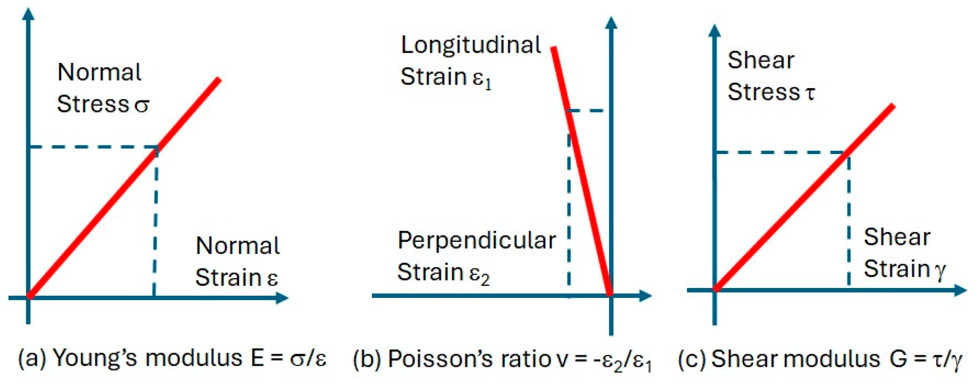
Figure 2.
Sinusoidal Stress and Strain graphs.
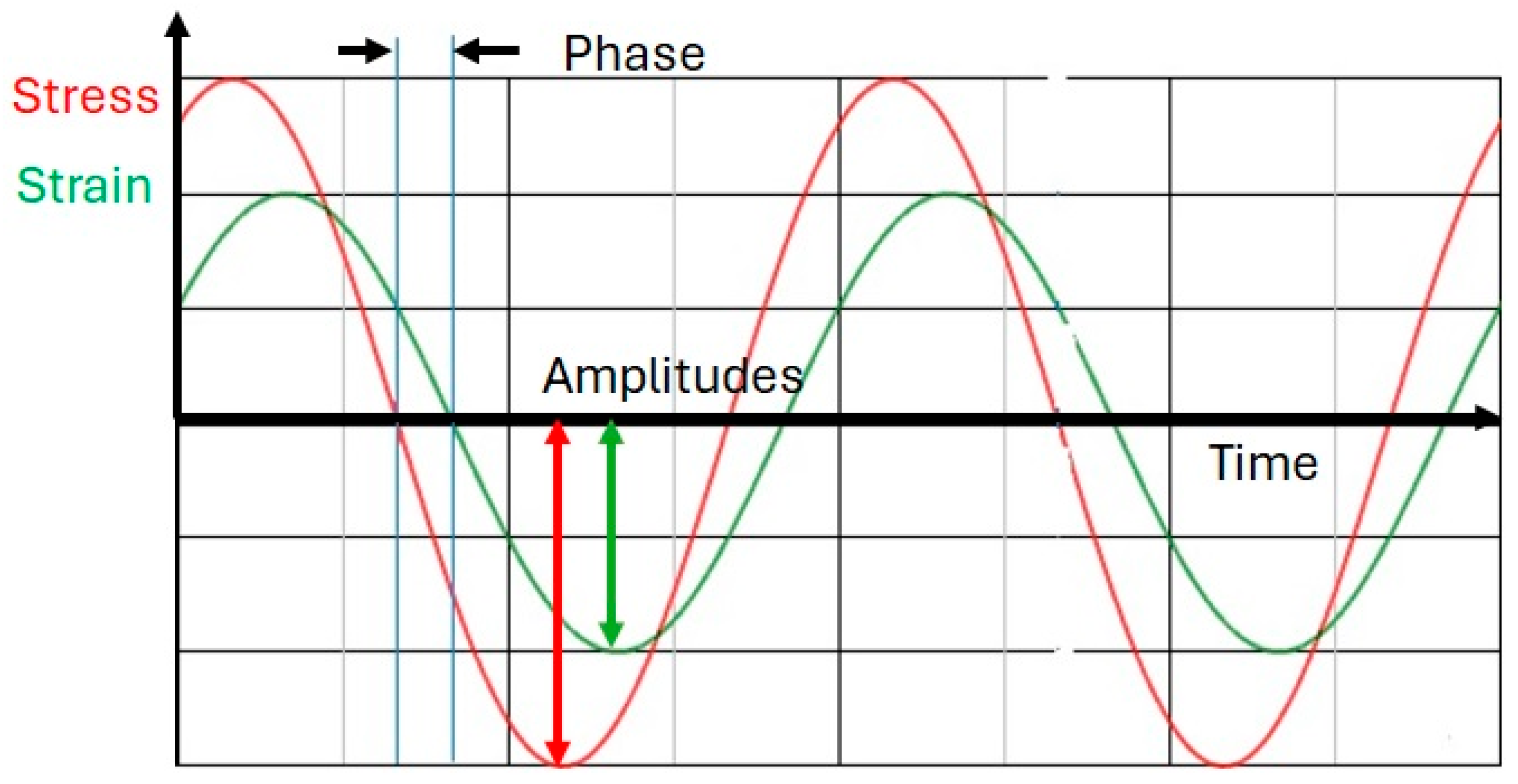
Figure 3.
Examples of sheets with orthotropic material directions (1, 2).

Figure 4.
Two test beams were cut along orthotropic directions 1 and 2, and a rectangular test plate with edges parallel to the orthotropic material directions.
Figure 4.
Two test beams were cut along orthotropic directions 1 and 2, and a rectangular test plate with edges parallel to the orthotropic material directions.
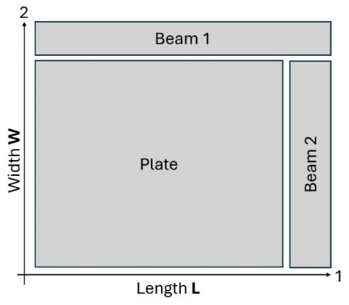
Figure 5.
First 5 Modal shapes of a Poisson plate.
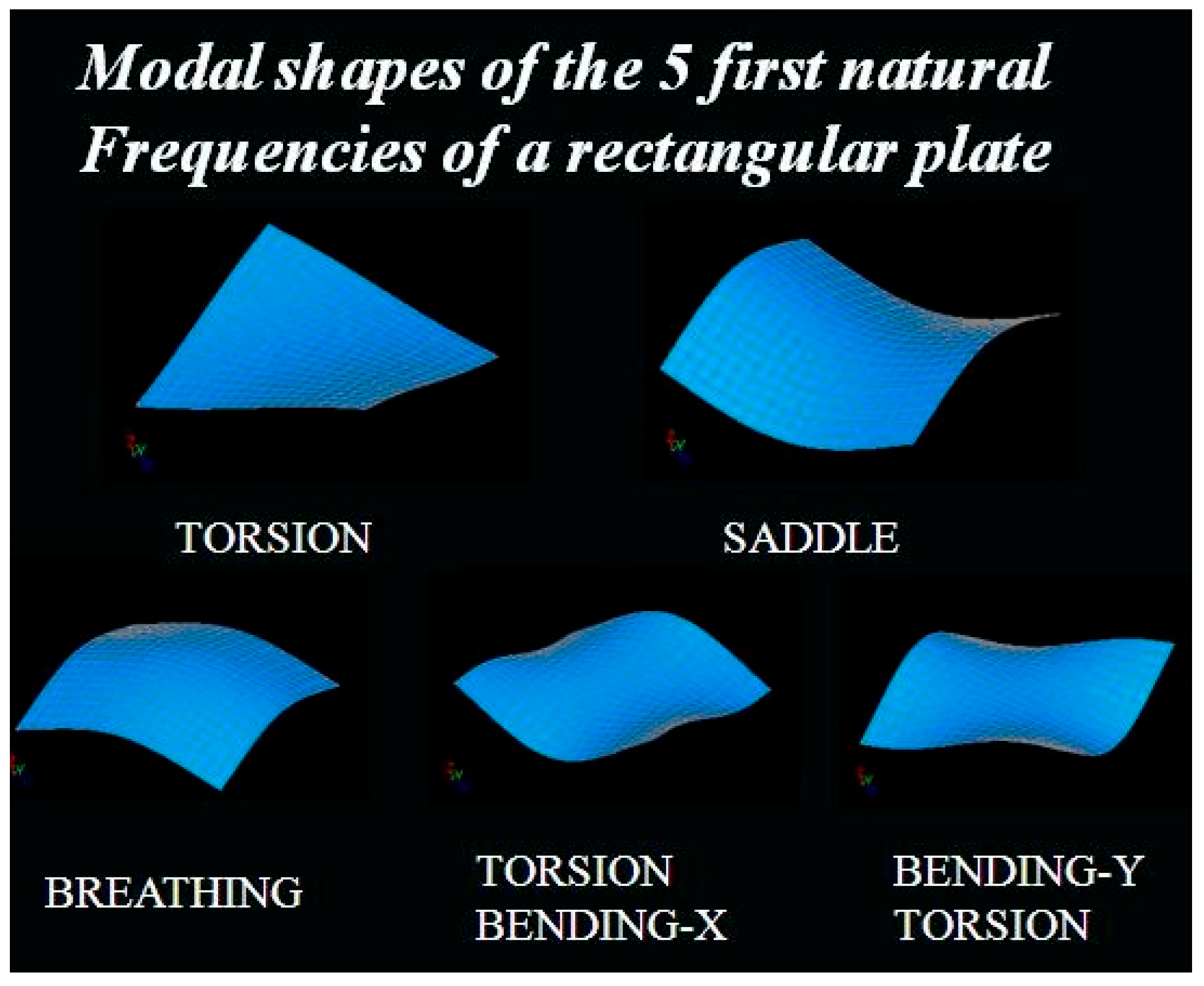
Figure 6.
Different stages of pendulum impact (figure taken partly from [28]).
Figure 6.
Different stages of pendulum impact (figure taken partly from [28]).
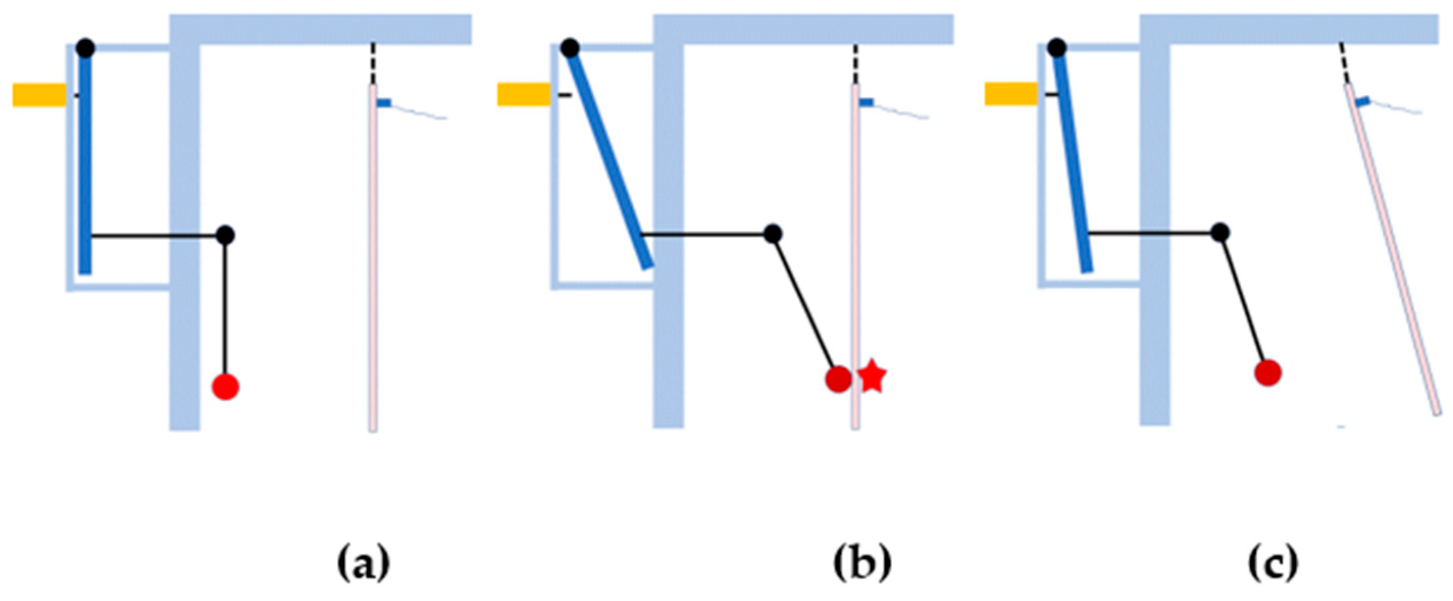
Figure 7.
Patches of glass (left) and Basalt (right) fabric (with millimeter scale).
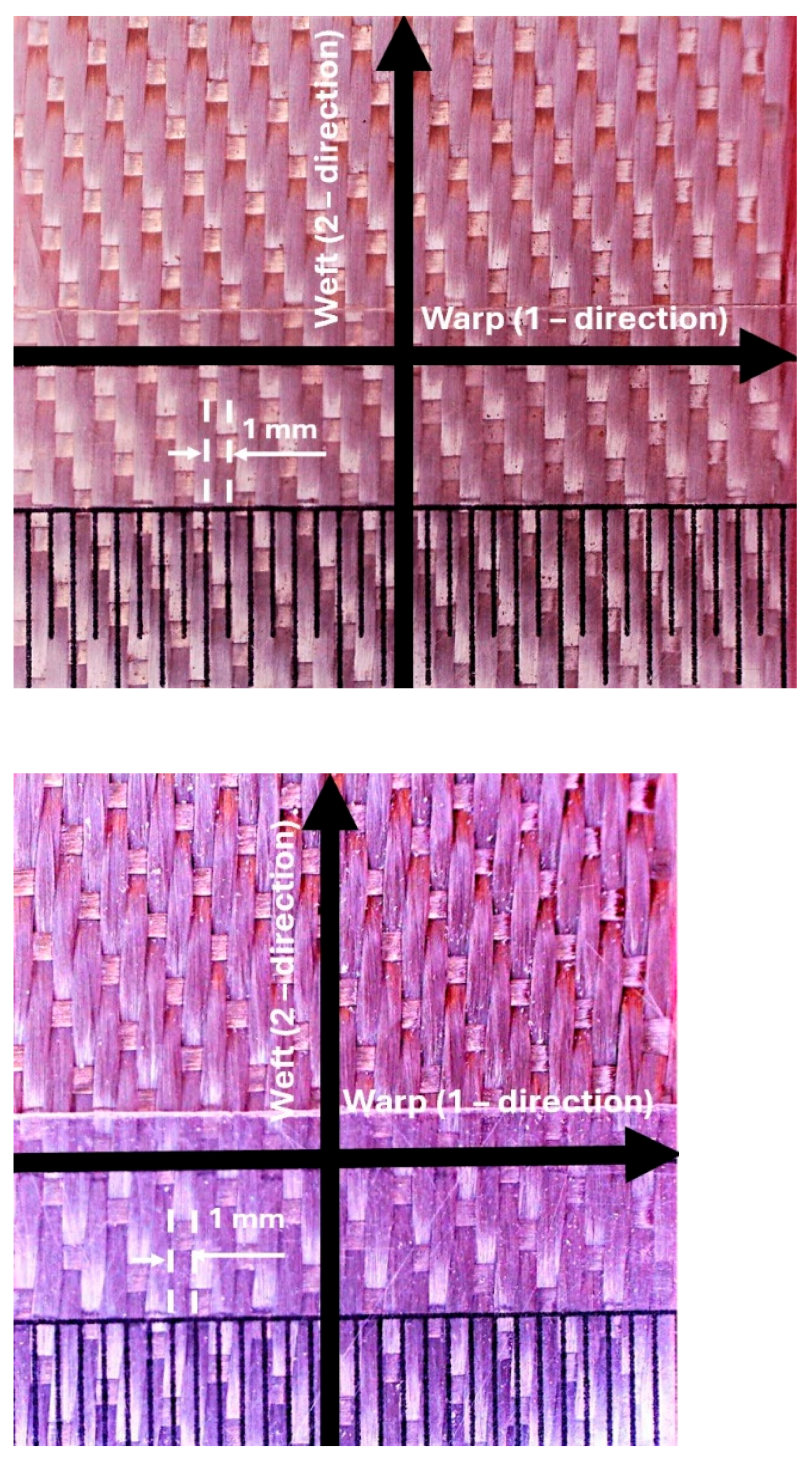
Figure 8.
Recorded Force-displacement graph during a 3-point bending test.
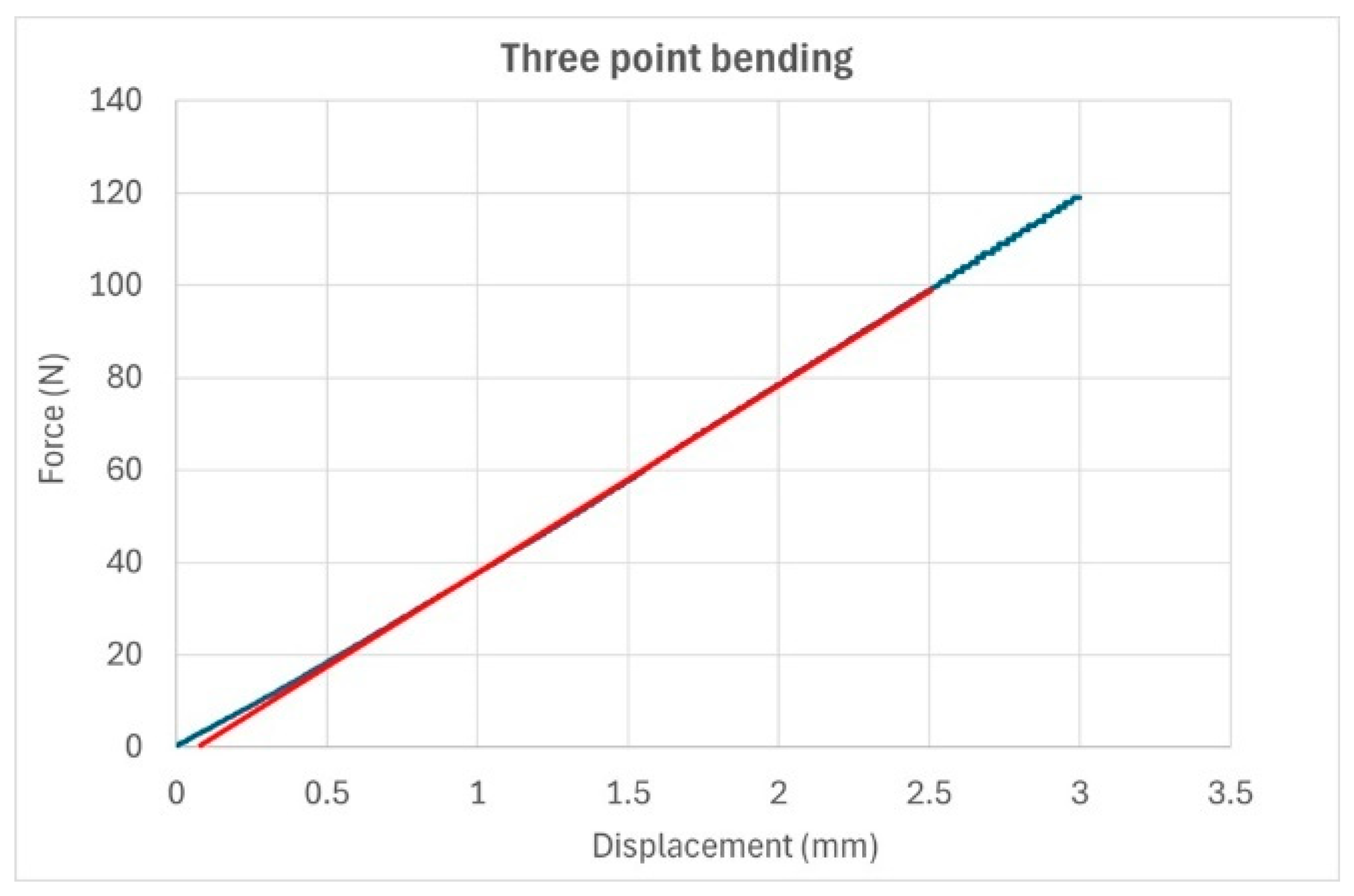
Figure 9.
Young’s modulus (in GPa) for BFRP and GFRP (3-point bending and standard IET results) as function of the temperature.
Figure 9.
Young’s modulus (in GPa) for BFRP and GFRP (3-point bending and standard IET results) as function of the temperature.
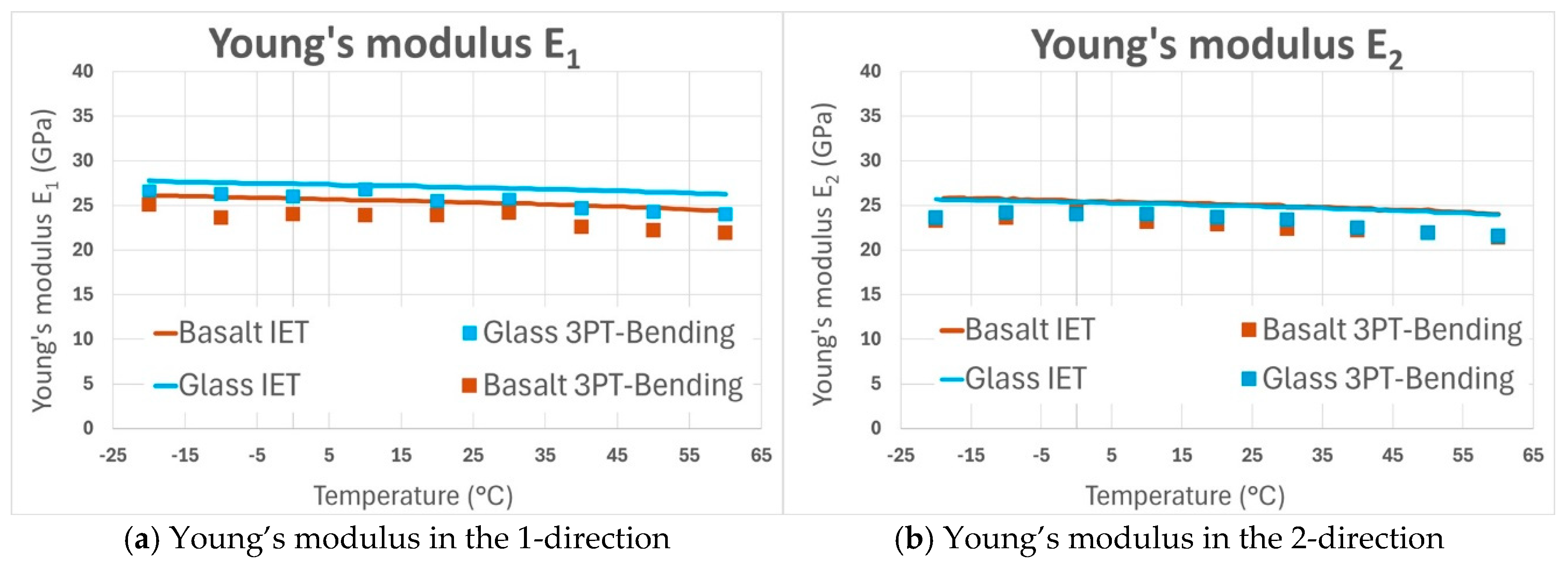
Figure 10.
Resonance frequencies in [Hz] of GFRP and BFRP samples measured with automated IET testing in the climate chamber between -20 °C and 60 °C.
Figure 10.
Resonance frequencies in [Hz] of GFRP and BFRP samples measured with automated IET testing in the climate chamber between -20 °C and 60 °C.
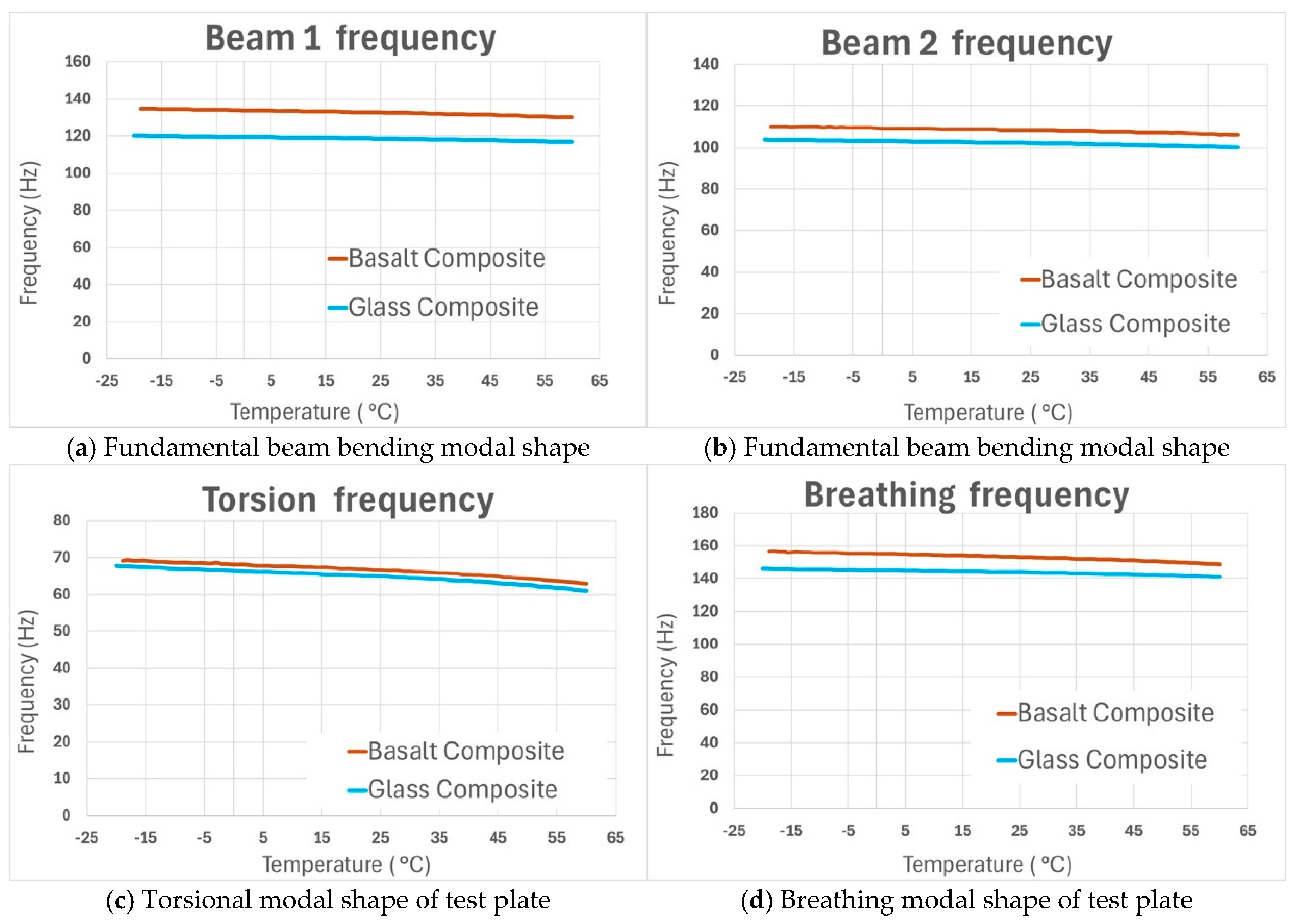
Figure 11.
Damping ratio in [%] plots of GFRP and BFRP samples measured with automated IET testing in the climate chamber between -20 °C and 60 °C.
Figure 11.
Damping ratio in [%] plots of GFRP and BFRP samples measured with automated IET testing in the climate chamber between -20 °C and 60 °C.

Figure 12.
Real part of the orthotropic engineering constants of GFRP and BFRP samples.
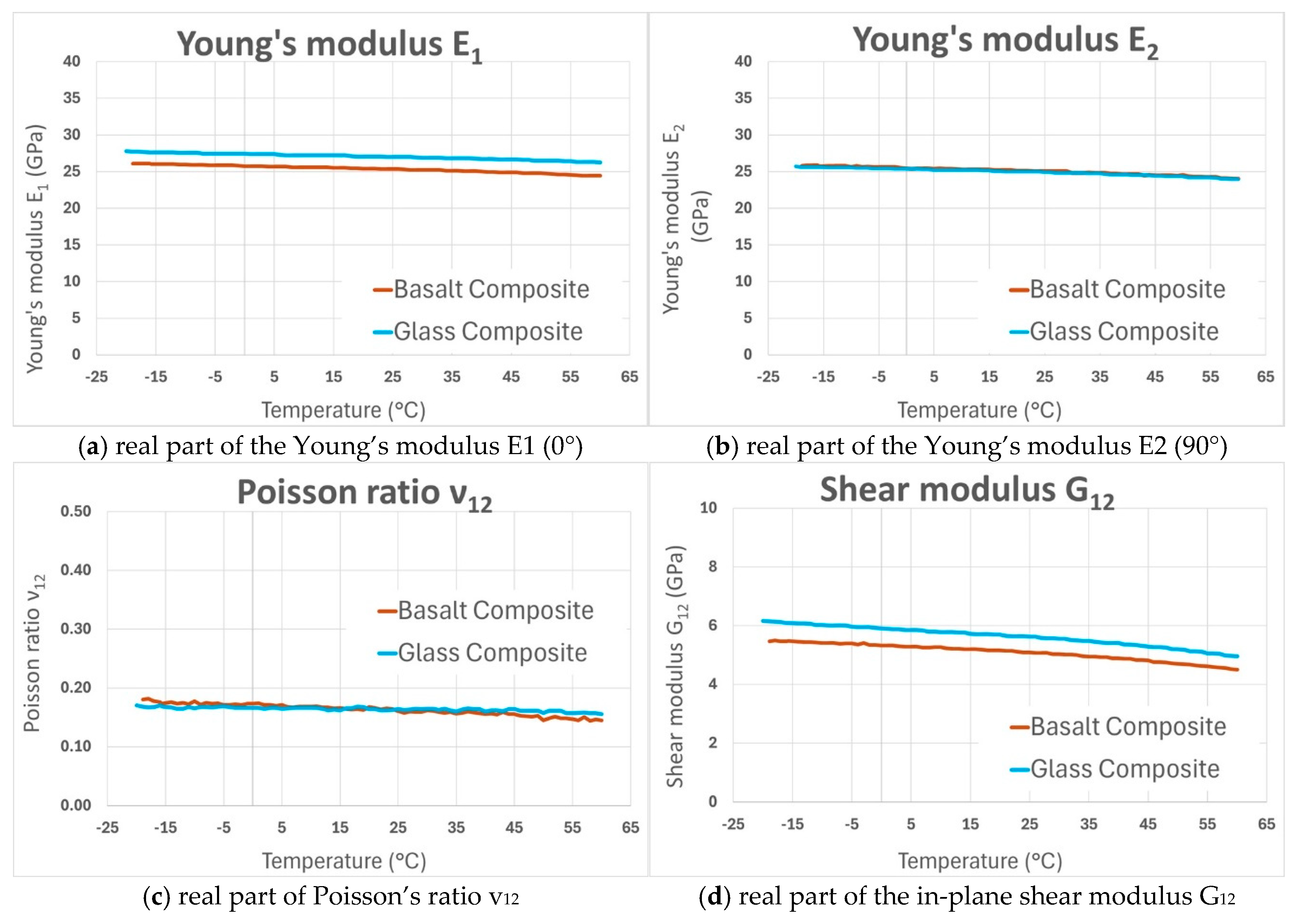
Table 1.
Dimensions and masses of the test beams and plates.
| Sample | Length [m] | Width [m] | Thickness [m] | Mass [kg] |
|---|---|---|---|---|
| GFRP Beam-1 (0°) | 0.255 | 0.0259 | 0.00200 | 0.0249 |
| GFRP Beam-2 (90°) | 0.272 | 0.0260 | 0.00203 | 0.0268 |
| GFRP plate | 0.243 | 0.234 | 0.00203 | 0.2170 |
| BFRP Beam-1 (0°) | 0.247 | 0.0260 | 0.00217 | 0.0262 |
| BFRP Beam-2(90°) | 0.273 | 0.0260 | 0.00217 | 0.0289 |
| BFRP plate | 0.243 | 0.0239 | 0.00223 | 0.2430 |
Disclaimer/Publisher’s Note: The statements, opinions and data contained in all publications are solely those of the individual author(s) and contributor(s) and not of MDPI and/or the editor(s). MDPI and/or the editor(s) disclaim responsibility for any injury to people or property resulting from any ideas, methods, instructions or products referred to in the content. |
© 2025 by the authors. Licensee MDPI, Basel, Switzerland. This article is an open access article distributed under the terms and conditions of the Creative Commons Attribution (CC BY) license (http://creativecommons.org/licenses/by/4.0/).
Copyright: This open access article is published under a Creative Commons CC BY 4.0 license, which permit the free download, distribution, and reuse, provided that the author and preprint are cited in any reuse.


