Submitted:
29 May 2025
Posted:
30 May 2025
You are already at the latest version
Abstract
This paper introduces and proves a novel proposition on the structural closure property of Linear Time-Invariant (LTI) invertible systems. Specifically, it demonstrates that systems composed by arbitrarily combining LTI invertible systems through cascade, parallel, and feedback configurations remain LTI invertible systems. Furthermore, a constructive approach is proposed to reinterpret systems governed by linear constant-coefficient differential equations, proving that under the assumption of causality, such systems are invertible. The theoretical contribution of this work enriches the understanding of invertibility in signal and system theory, while its practical value lies in providing structural support for the design and analysis of complex systems.
Keywords:
linear time-invariant (LTI)
; invertibility
; structural closure property
; constructive proof
MSC: 93C05; 93B05
1. Introduction
Signal and system theory, particularly in the context of engineering applications, focuses on the analysis of Linear Time-Invariant (LTI) systems. These systems are foundational in fields such as communication engineering, control theory, and system optimization [1,2,3,4]. Compared to nonlinear systems, LTI systems benefit from a well-established theoretical framework and unified analysis methods [5,6]. However, the concept of invertibility within this framework has received limited attention, often restricted to a few specific cases [7,8,9,10]. Table 1 summarizes typical examples of invertible and non-invertible systems, covering four categories: linear/non-linear and time-invariant/time-variant. In this table, denotes the input signal and the output signal.
The examples in Table 1 demonstrate that invertibility is independent of linearity and time-invariance. For instance, an ideal filter is an LTI system but is not invertible, as the original signal cannot be reconstructed from the filtered output signal [11,12]. Conversely, systems such as and form an inverse pair but are not LTI systems. However, the deeper relationship between LTI property and invertibility remains unclear, which is why invertibility has not been incorporated as a core concept in the theory of signals and systems.
This paper addresses this gap by exploring the relationship between the LTI property and invertibility from a structural perspective. Based on foundational results in the theory of signals and systems , it is known that LTI systems retain their LTI property under cascade and parallel connections [1,2,13,14]. Building upon this, we propose two key insights:
- Structural closure property of LTI systems: Systems constructed from simple LTI systems via cascade, parallel, or feedback configurations remain LTI systems.
- Structural closure property of LTI invertible systems: If the component systems are both LTI and invertible, the combined system preserves both the LTI property and invertibility.
Building on this foundation, this paper introduces a constructive method to reinterpret systems described by linear constant-coefficient differential equations. Traditionally, the LTI property of such systems is verified through formal proofs based on the mathematical definitions of linearity and time-invariance. In contrast, the constructive approach proposed here not only provides a structural explanation for the LTI property of differential equation systems but also reveals that causality in such systems inherently implies invertibility.
This paper is organized as follows: Section 2 defines invertible systems, elaborates on the fundamental results concerning the linearity, time-invariance, and invertibility properties of systems; Section 3 proves the structural closure property of LTI invertible systems; Section 4 applies these results to analyze systems governed by linear constant-coefficient differential equations.
2. Preliminaries
2.1. Definition of Invertible Systems
In the context of the theory of signals and systems, a system is defined as a mapping between input and output signals, denoted as:
where denotes the system operator acting on the input to produce the output .
Definition 1.
A system is said to be invertible if there exists an inverse system such that:
and
This means that whether the signal flows from input to output through , or from output back to input through , the original signal can be fully reconstructed. In other words, cascading the system with its inverse yields an identity system, where the output is identical to the input.
Informally, an invertible system ensures a one-to-one correspondence between inputs and outputs: different inputs yield different outputs. By contrast, a non-invertible system may map distinct inputs to the same output, or a single input to multiple outputs.
2.2. Two Lemmas on the LTI Property and Invertibility of Systems
Lemma 1.
The inverse of an invertible system is unique.
Proof.
Suppose a invertible system has two inverses, and . By the definition of an inverse system, we have:
Since equation (3) holds for any invertible system and any admissible input , it follows by the transitivity of equality that . Therefore, the inverse system is unique. □
Lemma 2.
For LTI systems and with unit impulse responses and , respectively:
(a) The cascade of the two LTI systems is also an LTI system, with unit impulse response:
(b) The parallel connection of the two LTI systems is also an LTI system, with unit impulse response:
(c) The feedback system, as shown in Figure 1, is also an LTI system, with input-output relationship:
where denotes convolution.
Remark 1.
Propositions (a) and (b) are standard results in the literatur [1,2,13,14], often presented as textbook content or exercises. For proposition (c), it is evident from Figure 1 that the relationship between the input and the output holds. Specifically, the two are related through convolution. Clearly, these propositions can be proved using the associativity, linearity, and time-shift properties of convolution. As the derivation is straightforward, it is omitted here for brevity
In summary, Lemma 2 establishes that systems formed by combining LTI systems through cascade, parallel, and feedback structures remain LTI systems.
3. Two Theorems on the Invertible Systems
Theorem 1.
If two systems are mutual inverses, they share the same linearity (or non-linearity) and time-invariance (or time-variance) properties. Specifically, if one system is LTI, its inverse system is also LTI.
Remark 2.
The proof for all four cases is similar. Here, we illustrate the case for LTI systems.
Proof.
As shown in Figure 2, let and be a pair of mutual inverses, forming a cascade system denoted by , where denotes the cascade operation. Suppose is an LTI system with unit impulse response . By the definition of invertibility, is the identity system, whose unit impulse response is . Since the identity system is also LTI, if were not LTI, then would not satisfy the LTI property—this is a contradiction. Therefore, must also be LTI. By the properties of convolution, the unit impulse responses satisfy: . □
Theorem 2.
Let and be two LTI invertible systems with impulse responses and , and their respective inverses and with impulse responses and , satisfying: , . Then the following conclusions hold:
(a) Invertibility of the Cascade System
The cascade system formed by and remains invertible, with inverse system . The unit impulse response of the inverse system is , The system structure is illustrated inFigure 3.
(b) Invertibility of the Parallel System
The parallel system formed by and remains invertible, with its inverse system realizable via a feedback configuration: serves as the forward path, and as the feedback path. The system structure is illustrated in Figure 4.
(c) Invertibility of the Feedback System
The feedback system formed by and (as shown in Figure 1) remains invertible, Its inverse system is a parallel system composed of and .
Proof.
The proof of (a): As shown in Figure 3, let and , where denotes the cascade operation. By Lemma 2(a) and Theorem 1, for any admissible input , the output of the system is:
Applying the associative and commutative properties of convolution, we obtain:
Therefore, is the inverse system of . □
Proof.
The proof of (b): As shown in Figure 4, let , where denotes the parallel operation. Define the system as , where denotes the identity system, denotes the cascade operation. The denominator in a rational expression implies the presence of a feedback path. corresponds to the feedback system with as the forward path and as the feedback path.
By Lemma 2(b), the output of for input is:
By Lemma 2(c), passes through to yield output :
Substituting equation (6) into equation (7), we get:
By the zero-input, zero-output property of LTI systems, it follows that . Thus, is the inverse system of . □
Furthermore, by the symmetry of the structure in Figure 4, if is used as the forward path and as the feedback path, the resulting feedback system is also the inverse system of .
By Lemma 1, and are equivalent systems. We verify this by comparing their input-output relationships.
For :
For :
Convolving both sides of equation (9) with and equation (10) with , we simplify to:
Therefore, , proving they are the same system.
Proof.
The proof of (c): Theorem 2(b) has established that the inverse of a parallel system can be realized through a feedback configuration. Essentially, this indirectly proves Theorem 2(c). For a more thorough understanding, we now present an alternative proof for the invertibility of the feedback system.
By Lemma 2(c), the input-output relationship of the feedback system (as shown in Figure 1) is:
where and are the impulse responses of and respectively.By Theorem 2(a) and 2(b), both and the composite system are invertible. Therefore, there exists a one-to-one correspondence between the input and output in the feedback system, proving its invertibility. □
Remark 3.
In summary, Theorem 2 establishes that the inverse of a cascade system is also a cascade system, the inverse of a parallel system is a feedback system, and conversely, the inverse of a feedback system is a parallel system. Therefore, any system constructed by combining LTI invertible systems via cascade, parallel, and feedback operations remains an LTI invertible system.
4. Discussion
4.1. Relationship Between Lemma 2 and Theorem 2
Lemma 2 establishes the closure property of LTI systems, stating that LTI systems remain LTI under cascade, parallel, and feedback combinations. Building upon this, Theorem 2 extends the result by introducing an additional invertibility constraint, showing that systems constructed from LTI invertible systems also retain invertibility. This theoretical framework provides a foundation for constructing complex systems from simpler components, embodying the essence of the scientific method. As Leibniz famously stated: “All thoughts can be broken down into a small number of simple ideas, and these simple ideas, combined according to certain rules, can form any complex idea—just like mathematical operations.” The results derived from Lemma 2 and Theorem 2 echo this principle, offering a systematic approach for system design and analysis.
4.2. Proof of Linearity and Time-Invariance for Linear Constant-Coefficient Differential Equation Systems
Consider the general form of a linear constant-coefficient differential equation system:
where is the input signal, and is the output signal. The task is to prove that this system is linear and time-invariant.
4.2.1. Proof by Verification
In the theory of signals and systems, linearity and time-invariance are typically verified by applying their respective mathematical definitions.
Let input signals and produce outputs and under system (13), respectively:
Multiplying (14) by a constant , and (15) by , then adding, we obtain:
Thus, the system confirms linearity.
For time-invariance, consider an input . By convolving both sides of (13) with a delayed impulse and invoking the differentiation property of convolution, we obtain, we obtain:
Thus, the system is time-invariant.
While this verification-based approach is logically rigorous, it does not reveal the structural mechanisms of the system. From an engineering perspective, such proofs are often considered unsatisfying.
4.2.2. Constructive Proof
System (13) can be decomposed into a cascade of two subsystems and :
As shown in Figure 5, and are composed of differentiators and amplifiers, implemented via cascade, parallel, and feedback configurations. By Lemma 2, both and are LTI systems; therefore, their cascade is also an LTI system.
Compared with the verification-based approach, the constructive proof reveals the internal structure of the system more intuitively, despite its initial complexity. This structural insight benefits system design and analysis. Indeed, this perspective naturally recalls Xu Guangqi’s (1562–1633) reflection on Euclid’s Elements: “Seemingly obscure, but ultimately clear; seemingly complex, but ultimately simple; seemingly difficult, but ultimately easy.” In innovative research, constructive methods are often superior to verification-based ones, as intuitive understanding typically precedes formal logical reasoning, and the constructive proof here provides a compelling illustration of this principle.
4.3. Are Linear Constant-Coefficient Differential Equation Systems Invertible?
4.3.1. The General Case
To disprove a proposition, it suffices to provide a counterexample. We examine two of the simplest cases derived from system (13).
First, consider the differentiator system :
From a strict theoretical perspective, this system is evidently non-invertible. For example, both and (where is a constant) yield the same output, making it impossible to uniquely determine the input from the output.
Second, consider the system :
This system is LTI, and its properties depend on the choice of unit impulse response. As long as the condition is satisfied, the unit impulse response is:
where is the unit step function. Table 2 summarizes the system characteristics under different unit impulse responses. Due to the non-uniqueness of , the causality and invertibility of the system are also undetermined.
4.3.2. The Case Under Causality Assumption
System analysis usually assumes causality, which encompasses the following three aspects:
- Causality of Signals: Physical signals typically emerge at a specific point in time, represented as , where is the unit step function. For simplicity, we often set , implying for .
- Causality of Systems: In the physical world, every effect must have a cause, and the cause precedes the effect. System outputs depend on current and past inputs, not future inputs. Thus, the output has the form , satisfying .
- Initial Rest Condition: The system starts from rest, i.e., . This state is analogous to the “chaos” state described in creation myths, such as the “formless void and darkness” in the Genesis or the “chaos like a chicken's egg” in the account of Pangu splitting heaven and earth in Chinese mythology. From the perspective of modern physics, ”chaos” state refers to a state of maximal entropy, extreme disorder and and absolute stasis.
Under these assumptions, the following propositions hold:
Proposition 1.
is equivalent to an integrator:
Proof.
By the fundamental theorem of calculus [15] and under the causality assumption, integrating the expression for yields:
Given the initial rest condition, the proposition is proved. □
Proposition 2.
The differentiator is invertible, and its inverse is the integrator.
Proof.
By the definition of invertible systems, we have:
Therefore, and are mutual inverses, and the proposition is proved. □
In addition, amplifiers are trivially invertible. Therefore, by Theorem 2 and the system structure shown in Figure 5, we conclude that linear constant-coefficient differential equation systems are invertible under the assumption of causality.
Moreover, due to the inherent symmetry of the mathematical structure, such systems are also invertible under anti-causal conditions. The causality of a system is not dictated by its mathematical equation alone, but rather by physical intuition and empirical observation. Linear constant-coefficient differential equation systems are typically mathematical abstractions of real-world physical systems (e.g., mechanical or electrical systems), which are inherently causal. Therefore, system analysis must consider the physical context in addition to the mathematical formulation; otherwise, conclusions may deviate from reality. This is akin to the creative process in literature and the arts—rooted in life, elevated beyond life, but ultimately returning to life.
Does an anti-causal system exist? The universe, or yuzhou in Chinese (with yu referring to the spatial dimensions and zhou referring to the temporal dimensions), is vast and boundless. In such a universe, events that defy everyday experience, though having an extremely small probability, may inevitably occur. While anti-causal systems of this kind might exist in certain regions of spacetime, they hold greater theoretical significance than practical value for us. For a better understanding of this perspective, consider the following illustrative analogy: Although the vast majority of celestial bodies (such as planets in the solar system and even galaxies in the Milky Way) exhibit counterclockwise rotation due to initial conditions during formation, clockwise-rotating celestial bodies are not prohibited by physical laws. In fact, such celestial bodies have been observed, albeit they are extremely rare and located at great distances.
4.4. Other LTI Systems Beyond Linear Constant-Coefficient Differential Equations
Although linear constant-coefficient differential equation systems form an important subclass of LTI systems, they do not encompass all LTI systems. For example, ideal filters and delay elements are not represented by such systems.
According to previous conclusions, an ideal filter is non-causal and non-invertible, and therefore cannot be described by linear constant-coefficient differential equations.
A delay element, on the other hand, is an invertible system, with its inverse also being a delay element. The respective impulse responses are and . However, one is a causal system, and the other is an anti-causal system. Since mutual inverse linear constant-coefficient differential equation systems must possess the same causality, delay elements cannot be represented by such equations.
Author Contributions
Conceptualization, W.W.; methodology, C.L.; writing—original draft, W.W.; writing—review and editing, C.L. All authors have read and agreed to the published version of the manuscript.
Funding
This research was funded by the Young Innovative Talents Project in Guangdong Province, grant number 2019KQNCX013.
Data Availability Statement
The original contributions presented in the study are included in the article, further inquiries can be directed to the corresponding author.
Conflicts of Interest
The authors declare no conflicts of interest.
References
- Oppenheim, A.V.; Willsky, A.S.; Nawab, S.H. Signals and systems, 2nd ed.; Prentice Hall: Englewood Cliffs, NJ, USA, 1996; pp. 12–29. [Google Scholar]
- Lathi, B.P. Linear systems and signals, 2nd ed.; Oxford University Press: Oxford, UK, 2004; pp. 15–22. [Google Scholar]
- Palani, S. Signals and systems, 2nd ed.; Springer: Berlin, Germany, 2022; pp. 11–20. [Google Scholar]
- Ulaby, F.T.; Yagle, A.E. Signals and systems: Theory and applications, 2nd ed.; Michigan Publishing Services: Ann Arbor, MI, USA, 2024; pp. 13–21. [Google Scholar]
- Wang, W.; Lei, C. Exploring superposition and homogeneity in “Signal and System” course. Adv. Educ. 2025, 15, 272–278. [Google Scholar] [CrossRef]
- Wang, W.; Lei, C. Exploring causality in “Signal and System” course. Adv. Educ. 2025, 15, 85–92. [Google Scholar] [CrossRef]
- Qu, C.; He, J.; Duan, X. 3DIOC: Direct data-driven inverse optimal control for LTI systems. arXiv 2024, arXiv:2409.10884. [Google Scholar]
- Poe, K.; Mallada, E.; Vidal, R. Invertibility of discrete-time linear systems with sparse inputs. In Proceedings of the 2024 IEEE 63rd Conference on Decision and Control (CDC), Milan, Italy, 16–19 December 2024. [Google Scholar]
- Mishra, V.; Iannelli, A.; Bajcinca, N. A data-driven approach to system invertibility and input reconstruction. In Proceedings of the 2023 IEEE 62nd Conference on Decision and Control (CDC), Singapore, Singapore, 13–15 December 2023. [Google Scholar]
- Zhang, M.; Dahhou, B.; Li, Z.-T. On Invertibility of an Interconnected System Composed of Two Dynamic Subsystems. Appl. Sci. 2021, 11, 596. [Google Scholar] [CrossRef]
- Yi, H.; Chang, F.; Tan, P.; Huang, B.; Wu, Y.; Xu, Z.; Ma, B.; Ma, J. Design of infinite impulse response maximally flat stable digital filter with low group delay. Sci Rep. 2025, 15, 11074. [Google Scholar] [CrossRef]
- R, A.; Samiappan, S.; Prabukumar, M. Fine-tuning digital FIR filters with gray wolf optimization for peak performance. Sci Rep. 2024, 14, 12675. [Google Scholar] [CrossRef]
- Zheng, J.; Ying, Q.; Yang, W. Signals and systems, 2nd ed.; Higher Education Press: Beijing, China, 2000; pp. 13–28. [Google Scholar]
- Wu, D.; Li, X. Analysis of signals and linear systems, 5th ed.; Higher Education Press: Beijing, China, 2019; pp. 24–41. [Google Scholar]
- Arnol’d, V.I. Huygens and Barrow, Newton and Hooke; Birkhäuser: Berlin, Germany, 1990; pp. 35–52. [Google Scholar]
Figure 1.
Structure of the feedback system.
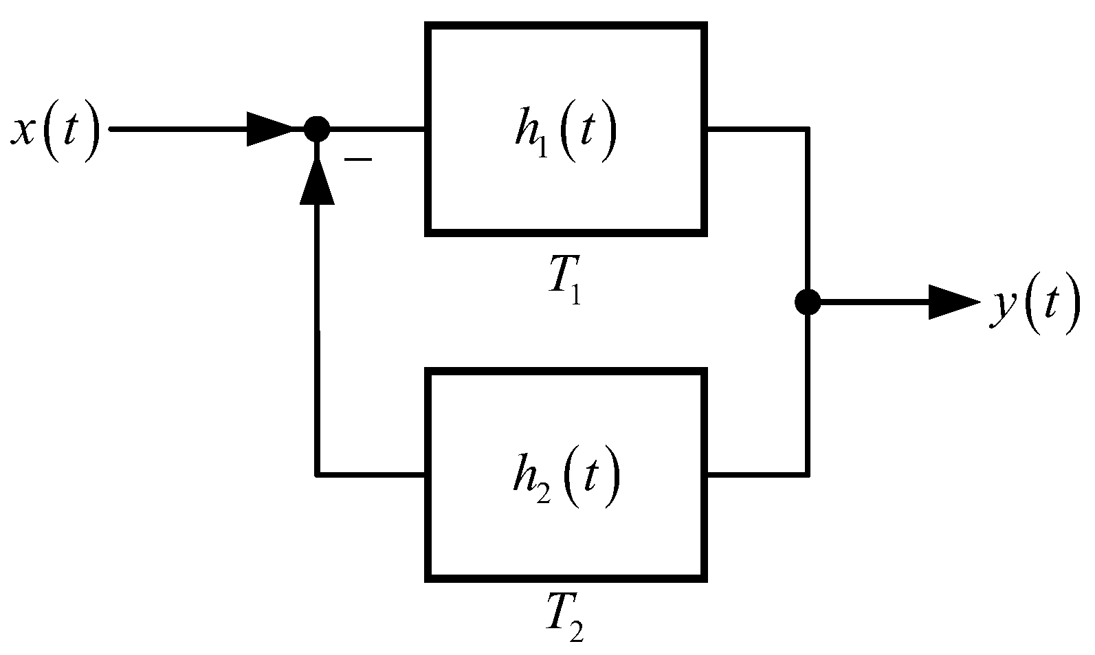
Figure 2.
Structure of the cascade system.
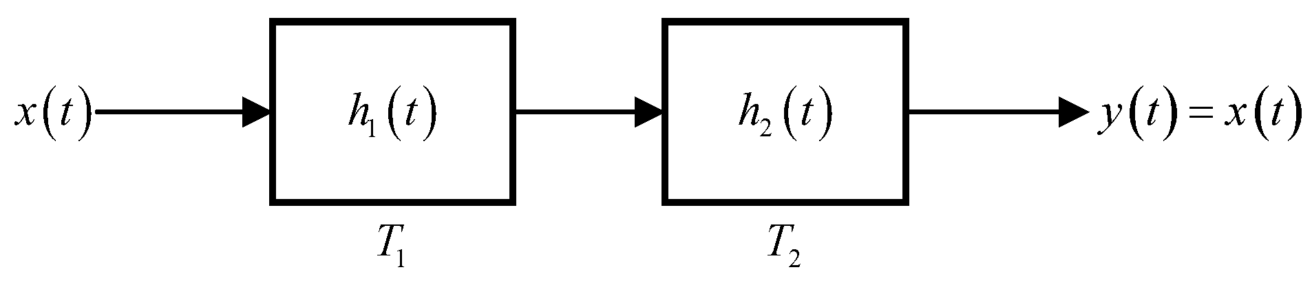
Figure 3.
Inverse system of the cascade system.
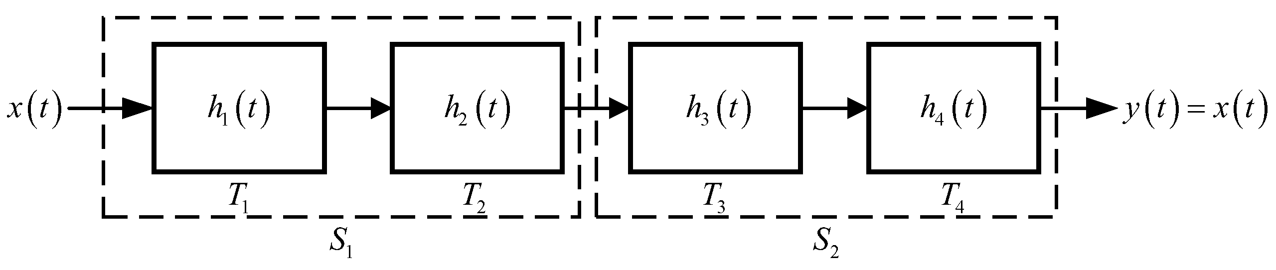
Figure 4.
Inverse system of the parallel system.
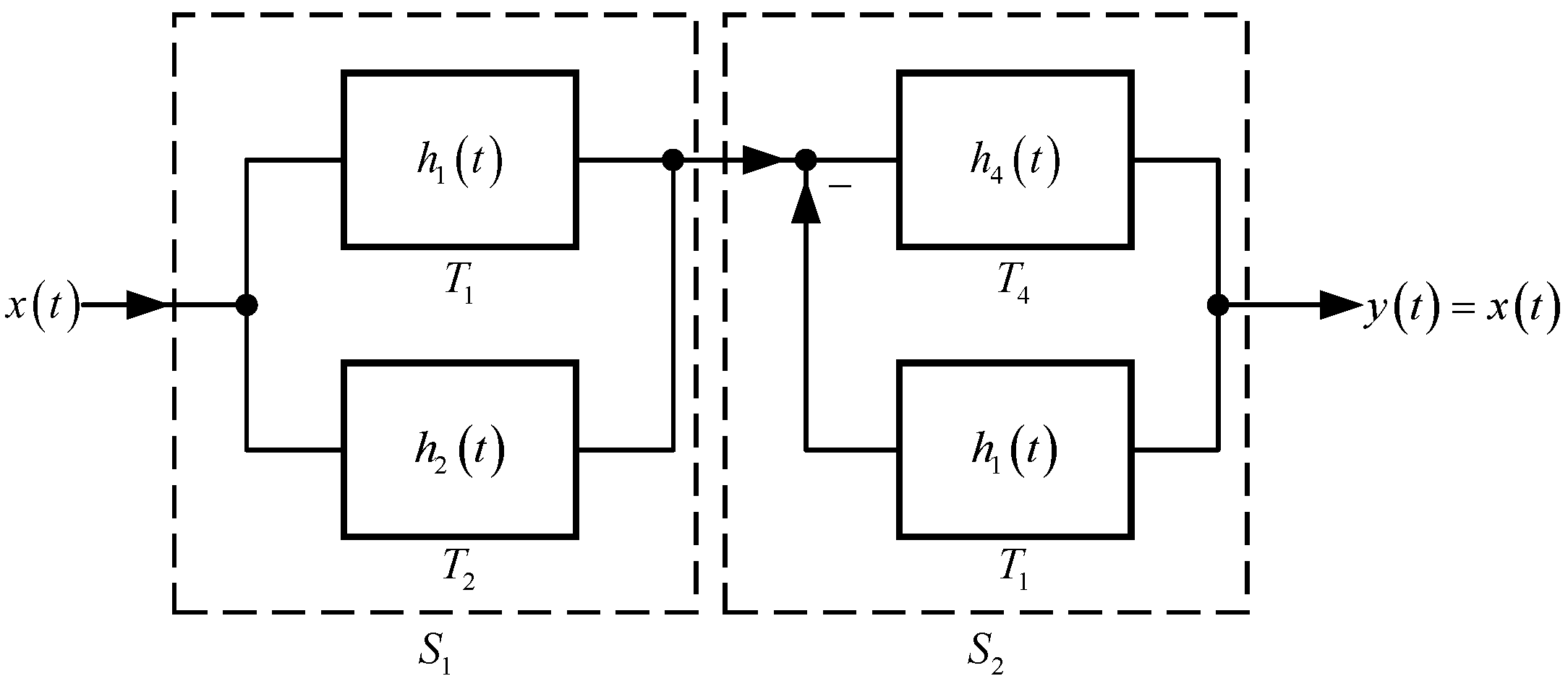
Figure 5.
Structural diagram of system (15).
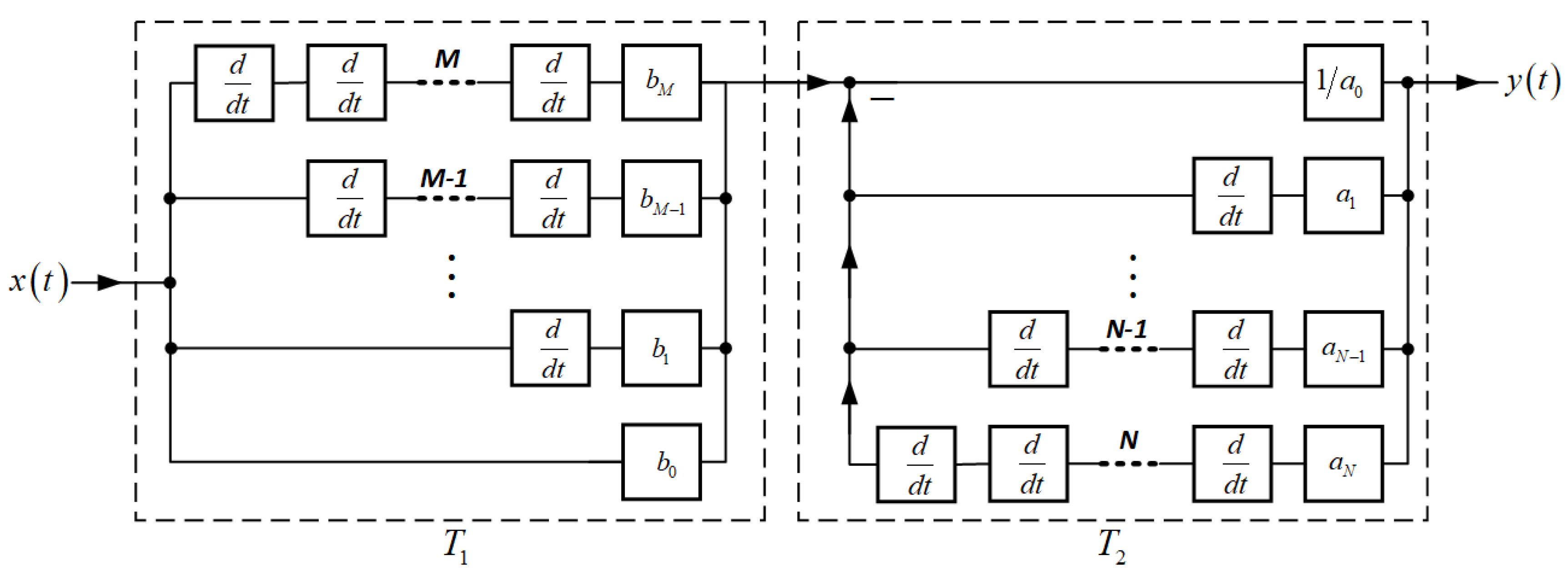

Table 1.
Examples of invertible and non-invertible systems.
| Category | Invertible system | Non-invertible system |
|---|---|---|
| Linear time-invariant | ||
| Linear time-variant | ||
| Non-linear time-invariant | ||
| Non-linear time-variant |
Table 2.
System properties under different unit impulse responses.
| System equation | Unit impulse response | System function | Causality | Invertibility |
|---|---|---|---|---|
|
, |
Causal | Invertible | ||
|
, |
Non-causal | Invertible | ||
| Not defined | Non-causal | Non-invertible |
Disclaimer/Publisher’s Note: The statements, opinions and data contained in all publications are solely those of the individual author(s) and contributor(s) and not of MDPI and/or the editor(s). MDPI and/or the editor(s) disclaim responsibility for any injury to people or property resulting from any ideas, methods, instructions or products referred to in the content. |
© 2025 by the authors. Licensee MDPI, Basel, Switzerland. This article is an open access article distributed under the terms and conditions of the Creative Commons Attribution (CC BY) license (http://creativecommons.org/licenses/by/4.0/).
Copyright: This open access article is published under a Creative Commons CC BY 4.0 license, which permit the free download, distribution, and reuse, provided that the author and preprint are cited in any reuse.


