Submitted:
29 May 2025
Posted:
30 May 2025
Read the latest preprint version here
Abstract
Ultra-high contrast (UHC) MRI is a term used to describe MR imaging that shows abnormalities with high contrast when little or no abnormality is seen on conventional MR images. It is achieved without the use of increased static or gradient magnetic fields. UHC can be accomplished by using tissue properties such as T1 twice or more in the same sequence to synergistically contribute to overall contrast as with directly acquired divided subtracted inversion recovery (dSIR) T1-bipolar sequences. These sequences also provide high contrast and high spatial resolution signal boundaries. UHC MRI can also be achieved by applying synthetic bipolar filters to high quality tissue property maps. Illustrative cases of mild traumatic brain injury, multiple sclerosis, methamphetamine substance use disorder, Parkinson's disease and white matter changes associated with a cerebral tumour are shown. Patients showed widespread abnormalities with directly acquired and synthetic dSIR sequences in areas where little or no abnormality was seen with conventional T2-wSE and/or T2-FLAIR sequences. New signs seen with dSIR sequences include the whiteout sign and grayout signs as well as the bilaminar cortex sign and bubble signs. dSIR and other bipolar sequences create high contrast from small changes in T1 as well as other tissue properties, and are complementary to conventional clinical sequences which create high contrast from larger changes in T1 and/or T2. Comparison is made with other sequences which use single or combined inversion recovery images. dSIR and other tissue property bipolar filter (BLAIR) sequences utilise sequences that already exist on most MR machines and are easy to implement.
Keywords:
Ultra-high contrast
; divided subtracted inversion recovery (dSIR) sequence
; logarithmic subtracted inversion recovery (lSIR) sequence
; bipolar filter (BLAIR)
; synthetic MRI
; tissue boundaries
; multiple sclerosis
; whiteout sign
; grayout sign
Introduction
Ultra-high contrast MRI is a term used to describe MR imaging that shows abnormalities with high contrast when little or no abnormality is seen using conventional state-of-the-art MRI sequences. It is achieved without the use of increased static or gradient magnetic fields. For soft tissues, Xray CT can be regarded as high contrast, conventional state-of-the-art MRI as very high contrast and MRI which shows abnormalities with obvious contrast when they are not seen with conventional MRI as ultra-high contrast (UHC) [1].
A common mechanism for achieving UHC MRI is synergistic contrast in which changes in a single tissue property such as T1 are used twice or more in the same sequence to increase contrast rather than just once which is the case with most conventional sequences [2]. An example is the divided subtracted inversion recovery (dSIR) sequence in which the signals from two inversion recovery (IR) sequences with different inversion times (TIs) are subtracted to increase the contrast produced by small changes in T1. This contrast is increased further by division of the subtraction by the sum of the signals from the two sequences [3].
Another way of achieving UHC MRI is to use a high quality single tissue property map such as a T1 or T2 map and retrospectively apply a shaped filter to the map. The filter can increase contrast in one or more domains of tissue property values and maintain anatomical detail in the rest of the image. This is unlike narrow windowing of images which, when used to increase contrast, is accompanied by saturation of the display gray scale at the upper and lower signal thresholds. Narrow windowing leads to loss of anatomical detail and limits the degree to which contrast can be increased by windowing.
The principal clinical focus of UHC MRI to date has been on small changes in tissue properties from normal that are insufficient to generate useful contrast with conventional state-of-the-art sequences. When abnormalities are already seen with high contrast using conventional sequences, there is no particular clinical gain in demonstrating them with even greater contrast. As a result, attention has been directed at normal or near normal appearing tissues as seen with conventional state-of-the-art imaging.
Small changes in T1 may produce obvious abnormalities with the dSIR sequence as illustrated in a case of mild traumatic brain injury (mTBI) in an 18-year-old male patient shown in Figure 1. No abnormality is seen on the T2-FLAIR image in the patient (Figure 1A). The dSIR sequence in a normal age matched control shows normal white matter in the cerebral hemispheres as low signal (dark) (arrows) in Figure 1B. The same dSIR sequence in the patient shows abnormal high signal in his entire white matter (arrows) (Figure 1C). High signal (light) well defined boundaries are seen between normal white and gray matter on the dSIR image in Figure 1B. These are less obvious in Figure 1C because of the high signal in the abnormal white matter.
High contrast abnormalities in white matter have been seen using dSIR T1-bipolar filter (BLAIR) images of the type illustrated in Figure 1 in areas where little or no abnormality has been seen with T2-FLAIR or T2-wSE sequences in cases of mTBI [4], multiple sclerosis (MS) [5], methamphetamine substance use disorder [6] and Grinker's myelinopathy [7].
The purpose of this educational review is to describe the basic physics underlying UHC MRI using BLAIR images and illustrate use of these images in patients in order to facilitate wider use of them in clinical practice.
Basic Physics
Tissue Property Filters (TP-Filters) and the Inversion Recovery (IR) Sequence
The first part of this paper is a condensed and updated version of work published previously [1,2,3]. It is included to make the paper self-contained and not require concurrent reference to other papers to understand the contrast of clinical images included in the paper.
Instead of illustrating image contrast in the usual way by plotting longitudinal and then transverse magnetisation (MZ and then MXY) against time using the Bloch equations as in Figure 2, it is possible to use plots of signals produced by the exponential recovery of longitudinal magnetisation and exponential decay of transverse magnetisation against T1 and T2 respectively (rather than against time). These plots are tissue property filters (TP-filters); the tissue properties may be mobile proton density, T1, T2, T2*, D*, etc [8,9]. In this paper the term tissue is used to include fluids unless otherwise specified.
For TR >> T1, the T1 dependent part of the IR sequence has the signal equation:
where ST1 is the signal from the T1-filter, TI in the inversion time and T1 is the longitudinal relaxation time. The T1-filter of the IR sequence (with a constant value of TI) is shown in phase-sensitive or signed form in Figure 3A where it is a monotonic low pass filter, and in magnitude form in Figure 3B where it is a negative unipolar filter. The maximum size of the slopes of these two filters are shown with red lines in Figure 3A and Figure 3B. The magnitude forms of the IR filter ST1 = (1-2e-TI/T1) for T1 <  and ST1 = (2e-TI/T1 -1) for T1 > are used in the subsequent text unless otherwise specified.
ST1 = 1-2e-TI/T1
and ST1 = (2e-TI/T1 -1) for T1 > are used in the subsequent text unless otherwise specified.When TI is increased, the magnitude IR T1-unipolar filter shifts to the right as shown in Figure 4. Figure 4A (left) shows the IR T1-filter with a short TIs (e.g., the Short TI IR or STIR sequence) for brain where gray matter (G) has a higher signal than white matter (W). The slope of the T1-filter between W and G is moderately positive (red line).
When the TI is increased to an intermediate TI, TIi, as in Figure 4B (centre), the T1-filter is shifted to the right. W and G are fixed in the same position on the X axis, and W now has a higher signal than G. The slope of the T1-filter between W and G is strongly negative (red line).
When the TI is increased further to a long TI, TIl, the T1-filter is displaced further to the right, as in Figure 4C (right) where W has a slightly higher signal than G, and the slope of the T1-filter between them is mildly negative (red line).
Using the small change approximation of differential calculus, the contrast (difference in signal) produced by each T1-filter from the increase in T1 from W to G (horizontal green arrows in Figure 4A, Figure 4B and Figure 4C) is the size of this increase multiplied by the slopes of the respective T1-filters (i.e. by their first derivatives, the red lines). This contrast is shown by the vertical blue arrows in Figure 4 and is moderately positive in Figure 4A, highly negative in Figure 4B and mildly negative in Figure 4C. The slopes of the T1-filters show the contribution of the sequence to contrast in each example.
Subtracted IR (SIR) and Divided Subtracted IR (dSIR) Bipolar Filters
Two conventional magnitude IR T1-unipolar filters with different TIs, namely TIshort = TIs and TIintermediate = TIi are shown in Figure 5A. The subtraction: first TIs T1-filter minus the second TIi T1-filter produces the subtracted IR (SIR) T1-bipolar filter shown in Figure 5B. The vertical dashed lines at the null points of the two IR T1-filters shown in Figure 5A divide the X axis in Figure 5B into the lowest Domain (lD), the middle Domain (mD) and the highest Domain (hD). In the mD in Figure 5B (between the two dashed lines) the size of the slope of the SIR T1-bipolar filter is about double that of the IR T1-filters shown in Figure 5A. This is because the slope of the SIR filter in its mD in Figure 5B is the positive slope of the TIs filter in the mD shown in Figure 5A minus the negative slope of the TIi filter in the mD also shown in Figure 5A.
The two IR T1-filters shown in Figure 5A can also be added to give the Added IR (AIR) T1-filter shown in Figure 5C. In its mD, which is bounded by the vertical dashed lines, the signal is reduced to about 0.20 compared with its value of 2 at T1 = 0 (i.e. about one tenth).
Figure 6A shows a divided SIR (dSIR) T1-bipolar filter in which the SIR T1-bipolar filter in Figure 5B is divided by the AIR T1-filter in Figure 5C i.e. . The signal (SdSIR) of the dSIR filter is given by:
 where STIs is the signal from the shorter TI filter and STIi is the signal from the intermediate TIi filter.
The resulting dSIR T1-bipolar filter (Figure 6A) shows a negative pole and a positive pole. Its mD shows a highly positive nearly linear slope which is about ten times greater than the slopes of the IR T1-filters shown in Figure 5A. The dSIR filter has maximum and minimum values of ±1. (The contributions from mobile proton density and T2 to conventional IR sequences cancel out with dSIR sequences which are therefore T1 maps; the whole sequence can be accurately represented by its T1-bipolar filters.)
Figure 6B compares the contrast produced by a conventional STIs IR T1-unipolar filter (pink) to that from the SIR T1-bipolar filter (blue) shown in Figure 5B from the same increase in T1 (horizontal positive green arrow, ΔT1). ΔT1 is multiplied by the slopes of the respective STI IR and SIR filters (red lines) to produce the differences in signal ΔS, i.e. the contrast from each of them. These are shown by the vertical pink and blue arrows on the right. The SIR T1-bipolar filter generates about twice the contrast (blue arrow) of the STIs IR T1-unipolar filter (pink arrow) from the same increase in T1, ΔT1.
Figure 6C compares the contrast produced by the STIs IR T1-unipolar filter (pink) to that produced by the dSIR T1-bipolar filter shown in Figure 6A (blue). The increase in T1 (horizontal positive green arrow, ΔT1) is multiplied by the slopes of the respective STIs IR and dSIR filters (red lines) to produce the differences in signal ΔS, or contrast generated by the two filters. These are shown by the vertical pink and blue arrows on the right. For the same increase in T1 (ΔT1), the dSIR T1-bipolar filter produces about ten times greater contrast than the STIs IR T1-unipolar filter. The STIs IR T1-filter is that of a conventional TI IR sequence such as MP-RAGE (magnetisation prepared-rapid acquisition gradient echo).
To produce the large increase in contrast shown in Figure 6C, the dSIR sequence is typically targeted at the small increase in the T1 of normal tissue produced by disease (shown by the horizontal green arrow) and this is positioned within the steeply sloping mD of the dSIR T1-bipolar filter. This is done by choosing appropriate values of TIs and TIi. The target is often small increases in the T1 of white matter. High contrast can also be produced by difference or change in T1 within the lower part of the hD and the upper part of the lD where the dSIR T1-bipolar filter has relatively steep slopes. More detail is available in reference [3].
Contrast at Tissue Boundaries
MRI tissue boundaries take different forms such as a gradual change in signal from one tissue to another as well as sharply defined high and low signal boundaries between tissues. In the boundary region between two pure tissues (such as between white and gray matter) the T1s of voxels which contain mixtures of the two tissues typically span the range of T1 values between those of the two pure tissues. If a narrow mD dSIR T1-bipolar filter (e.g., with TIs nulling normal white matter, and TIi longer than TIs but less than that needed to null gray matter) is used there are mixtures of the two pure tissues in voxels in the boundary region with intermediate T1 values (T1W,G) which correspond with the peak of the T1-bipolar filter as shown in Figure 7. This produces a high signal boundary between white matter and gray matter. The dSIR T1-bipolar filter shows much higher contrast than that produced between white matter and gray matter by a conventional white matter nulled IR sequence such as MP-RAGE (Figure 7). The mechanism shown in Figure 7 produces the high signal SW,G at the boundary between normal white and normal gray matter shown in Figure 1B. High spatial resolution boundaries are also seen at the junction between CSF and white matter at ventricular boundaries, and can be seen at the boundary between gray matter and CSF with wide mD sequences [3]. The high and low signal boundaries on dSIR images are iso-T1 contours.
T1 Maps and Qualitative - Quantitative MRI
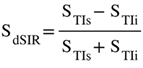
To better understand the dSIR T1-bipolar filter, a linear equation of the form y = mx + c can be used to approximate the filter in its mD. The equation is produced by fitting a straight line between the first and last points of the mD (i.e. first point x = and y = -1, and last point x = and y = +1). In the mD, the signal of the dSIR sequence SdSIR, is given by:
where ΔTI = TIi - TIs (i.e., second TI minus first TI) which is positive, and ΣTI = TIs + TIi which is also positive. Note that because ΔTI is positive, the slope is positive. The offset is negative.
The expression in Eq. (2) illustrates four key features of the dSIR T1-bipolar filter, firstly, the near linear change in signal (i.e. SdSIR) with T1 in the mD, secondly, the filter has a slope in the mD equal to , thirdly the filter shows high sensitivity to small changes in T1 when the size of ΔTI is small. When ΔT1 is small, the size of ΔTI can be decreased to match it and so scale up the sensitivity of the filter. The reduction in ΔTI increases the steepness of the T1-filter in the mD and thus the amplification of contrast produced from ΔT1. This compensates for the small value of ΔT1 until the sequence becomes SNR and/or artefact limited. This is not the case with conventional IR sequences where, if ΔT1 is decreased, contrast decreases.
Fourthly, Eq. (3) can be used to calculate T1 values in the mD so that:
The linear approximation is only valid in the mD. Also, it is assumed that TR is long compared to tissue T1 values. An equivalent expression that allows for incomplete recovery of longitudinal magnetisation during TR can be formulated.
Outside of the mD in the lD and hD, the magnitude of the dSIR T1-bipolar filter signal decreases towards zero at minimum and maximum values of T1. T1s in the mD occupy the full range of the display gray scale from black to white. T1s from the shortest and longest T1s in the lD and hD respectively only occupy parts of the display gray scale.
Log Then Subtracted Inversion Recovery (lSIR) Sequences
Another bipolar filter is the natural logarithm (ln) then subtracted inversion recovery (lSIR) filter [10]. The signal of this filter (SlSIR) is half of the subtraction: ln short STIs T1-filter minus ln intermediate STIi T1-filter. The ln STIs and ln STIi unipolar negative T1-filters are shown in Figure 8 and have sharper negative poles than those of unipolar STIs and STIi T1-filters shown in Figure 5A.
Figure 9 shows a dSIR T1-bipolar filter in blue and the corresponding lSIR T1-bipolar filter with the same TIs in orange. The two filters appear similar in the lowest region of the lD and in the highest region of the hD as well as in the central region of the mD. The slope of the dSIR filter is essentially constant and equal to . The magnitude of the slope of the lSIR filter is the same that of the dSIR filter at the centre of the mD but greater around the lower and higher nulling TI values. The lSIR filter asymptotically approaches negative and positive infinity at the two corresponding T1s. The lSIR filter increases its contrast amplification as the change in T1 from normal becomes smaller. Like the dSIR filter, the lSIR filter essentially eliminates the mobile proton density and T2 dependence of the full IR sequence and so can be used to model the full sequence behaviour.
The lSIR filter is an inverse hyperbolic tangent of the dSIR filter in the mD (SlSIR = atanh SdSIR), and an inverse hyperbolic cotangent of the dSIR filter in the lD and hD.
From a practical point of view, the lSIR T1-filter has 2-3 times the slope of the dSIR T1-filter for very small differences or changes in T1 around the null points and thus has 20-30 times greater contrast than conventional IR sequences for the same very small differences or changes in T1. The maximum and minimum values of the lSIR filter are usually shown as ±2-3 (rather than ±infinity). This compares with values of ±1 for the dSIR filter. The low and high signal boundaries of the lSIR filter are narrower than those of the corresponding dSIR filter.
The lSIR filter shows a selective increase in slope, or sharpening, at iso-T1 contours close to the nullpoints. It is not generalised edge enhancement of all boundaries on an image.
Composite (c) Bipolar Filters (T1 as Well as T2, T2*, D*, χ and/or MT)
It is possible to introduce an attenuation filter SOF (other filter) and apply it to one of the two IR filters used for dSIR T1-bipolar filter imaging in Figure 5 and Figure 6. SOF may equal e–ΔTE/T2, e–ΔTE/T2* or e–ΔbD* which introduce T2, T2* and D* dependence respectively. This provides additional contrast to the T1 contrast of the dSIR bipolar filter. When ΔTE equals zero, or Δb equals zero, SOF = 1. If SOF is set to 0.5 and 0.25, the curves shown in Figure 10A and Figure 10B result when using a narrow mD dSIR sequence (TIs = 350 ms and 500 ms). The nulling times are the same for all values of SOF.
In Figure 10A attenuation of the first IR filter (with TIs) is shown with SOF set at 1 (blue), 0.5 (orange) and 0.25 (yellow). The yellow and orange curves are wider around the outside of the first (negative) pole at the first TIs and are narrower and inside the second (positive) pole at TIi. This results in a broadening and loss of contrast and lower signal white matter around the first negative pole as well as increased contrast and narrower boundaries between white and gray matter around the positive pole. SOF can be set negative values to reverse the sign of the relevant contrast and make it synergistic with the T1 contrast.
In Figure 10B, attenuation of the second IR filter (with TIi) is shown. As SOF is decreased from 1.0 to 0.5 and 0.25, the filter narrows around the first (negative) pole and widens around the second (positive) pole. The negative contrast produced for the same difference in T1 is increased around the first negative pole. Composite (c) forms of the bipolar filters can be designated as cSIR, cdSIR, clSIR etc.
Susceptibility and magnetisation transfer can also be used to attenuate signals and produce supplementary contrast. The combination of T1 and T2* contrast may be of particular value in demonstrating the central vein sign and paramagnetic rim sign in multiple sclerosis (MS) as well as late sequelae of haemorrhage and fMRI in combination with perfusion.
Synthetic dSIR and lSIR T1-Bipolar Filter Images
Synthesizing Narrower mD Images from Wider mD dSIR and lSIR T1-Bipolar Filter Images
It is possible to synthetically create narrower mD dSIR images from wider mD dSIR images using Eq. 1 and the relationships illustrated in Figure 6A. The TIs of the narrower mD images are within those of the wider mD when using magnitude forms of the IR sequences.
Synthesizing dSIR and lSIR T1-Bipolar Filter Images from T1 Maps
dSIR and lSIR T1-bipolar filter images with particular values of TI can also be synthesised from T1 maps using Eq.1 and the relationships shown in Figure 6A, Figure 8 and Figure 9. T1 and other tissue property maps (T2, T2*, D*) have linear TP-filters with maximum signal values at the high end of the tissue property X axis. As a result, CSF has high signals on the maps and this can dominate their appearance. The problem can be avoided when appropriate T1-bipolar filters are applied to T1 maps to create T1-bipolar images in which CSF signal is reduced. The equivalent mapping using MP2RAGE acquisitions has also been described previously. While in principle the same contrast is obtained, there are wide discrepancies in the T1s measured by different techniques suggesting T1 is not independent of the method of acquisition. The unaccounted variance may mask small white matter abnormalities observed using dSIR images that were not previously seen with general purpose T1 mapping.
Synthesizing T2-, T2*-, D*and χ-Bipolar Filter Images Using Purpose Designed Bipolar Filters Together with T2, T2*, D* and χ Maps
It is also possible to create TP-bipolar filter images from tissue properties other than T1 using purpose designed synthetic TP-bipolar filters. These filters are typically based on the appearance of the dSIR T1-bipolar filter shown in Figure 6A and Figure 6C. They can have a linear function in their mD and a scaled reciprocal function (e.g., y = ) or similar function in their lDs and hDs. These functions join the linear function in the mD at signal values of -1 and +1, respectively. Synthetic TP-bipolar filters can then be used with T2, T2*, D* and χ maps to create T2-, T2*-, D*-and χ-bipolar filter images.
The lSIR inverse hyperbolic tangent and cotangent functions can also be used in the same way to create synthetic lSIR TP-bipolar filter images from tissue property maps.
Directly acquired T1-bipolar filter images and synthetic T1-, T2-, T2*-, D*-, χ- and MT-bipolar images with different TPs can be multiplied together to produce synergistic multi TP-bipolar filter images. Under log then subtraction (lSIR) the multiplicative contrast become additive. The signs of the slopes of the TP-bipolar filters (negative or positive) can be matched with the signs of the changes in tissue properties (negative or positive) to ensure the contrast produced by the different tissue properties is synergistic [2].
Window Levels and Widths of Displayed Images
Conventional Changes in Window Level and Width of MR Images
When an image is displayed, the window level sets the brightness (signal level) and the window width sets the contrast (signal difference). Changes in the window level and width of images change their signals on the gray scale display from S to SD and can be described using a high pass filter as seen in Figure 11A. This plots the display signal SD against the image signal S. This is a signal (S) filter not a TP-filter. Contrast (the difference in signal between the SDs of P and Q) may be increased by narrowing the window width as shown in Figure 11B so that P and Q are now respectively shown at the bottom and top ends of the display scale. With narrow windowing, signals with values at the upper end of the X axis from Q and beyond are all shown with the same high value of SD. As a result, there is no contrast between these voxels and they coalesce into blocks. This leads to a loss of anatomical coherence. The same also happens at the lower end of the S scale where values of S less than P have the same signal in Figure 11B and coalesce. This saturation of signals establishes a practical limit to how tightly images can usefully be windowed (i.e., how narrow the window width can usefully be made) and thus how much the contrast of the displayed image can be increased before the loss of anatomical coherence leads to a lack of credibility of the images. This is in addition to limits imposed by SNR considerations and image artefact levels.
dSIR Images
dSIR images can decrease ΔTI and so increase contrast. Maximum and minimum values are shown as high and low signal boundaries as in Figure 11C, T1 values lower than the lower nulling T1 value and greater than the greater nulling T1 value do not appear on the same plateaux as with conventional narrow windowing in Figure 11B, but vary in signal because of the sloping regions in the lDs and hDs of the dSIR T1-bipolar filter (Figure 11C). As a consequence, contrast is maintained and anatomical detail is preserved in all three Domains when ΔTI is decreased. As a result, contrast can be increased by decreasing ΔTI until it becomes SNR and/or artefact limited.
Methods
With approval from the New Zealand Health and Disability Ethics Committee 20/CEN/246 (26 June 2020), 21/CEN/246 (1 May 2021); 20/NTB/14 (21 May 2020); UAHPEC 018466 (20 Dec 2019); and the Northern B Health and Disability Ethics Committee 2022 EXP 13106 (18 Nov 2022) as well as informed consent from each subject, MR scans were performed on four adult normal controls, seven adult patients with mild traumatic brain injury (mTBI), MS, methamphetamine substance use disorder, Grinker's myelinopathy, Parkinson's disease and white matter in a patient with a glioma. The research was conducted in accordance with the Declaration of Helsinki. 3T scanners (General Electric Healthcare Premier and Siemens Healthineers Skyra) were used. 2D IR FSE sequences were performed with a TIs chosen to null the shortest T1 normal white matter (or slightly shorter) and a longer TIi chosen to produce narrow mD dSIR images targeted at small increases in the T1 of white matter from normal as illustrated in Figure 6C. 3D wide mD dSIR images with a short TIs and a long TIl were also obtained [5]. Longer TE 2D IR images were acquired to produce cdSIR images. Positionally matched 2D and 3D T2-FLAIR images were obtained as well as susceptibility weighted filtered images as described in Table 1.
Illustrative Cases
Mild Traumatic Brain Injury (mTBI)
Conventional MRI images usually show little or no change in mTBI but narrow mD dSIR images frequently show extensive high signal areas in white matter (the whiteout sign) (Figure 1). This may resolve within as little as two days or persist over years. It is generally attributed to neuroinflammation but oedema, demyelination and degeneration may also have a role.
In addition to the whiteout sign, there may be loss of contrast in the gray matter of the thalamus due to an increase in T1. This is manifest as a low contrast appearance between the medial and lateral thalamus (Figure 12A) (arrows) (a grayout sign). After remission normal high gray white matter contrast is restored (Figure 12B) (arrows). Contrast between the lateral thalamus (arrows) and the posterior limb of the internal capsule (PLIC) is low in (Figure 12A) but very high in (Figure 12B). The low contrast between the thalamus and the PLIC in (A) results from a reduction in signal in the gray matter of the lateral thalamus due to an increase in its T1 in the hD as well as an increase in signal in the white matter of the PLIC due to an increase in its T1 in the mD. This is reversed in (Figure 12B) where the normal high contrast boundary is restored.
Figure 13A shows a normal control with obvious contrast between the heads of the caudate nuclei and the adjacent CSF as well as between the cortex and CSF. Figure 13B shows a patient with mTBI who has a whiteout sign. There are grayout signs in the thalamus and putamen. In addition, contrast is lost between the heads of the caudate nuclei and CSF as well as between cortex and CSF which appear isointense. These are grayout signs. Thus, the patient has a combination of whiteout and grayout signs.
Multiple Sclerosis (MS)
Focal lesions, as well as patchy white matter changes, may be seen in areas that appear normal on T2-wFSE images in a patient in remission (Figure 15) (compare with normal low signal appearance of normal peripheral white matter in Figure 1B). In another case during a relapse, one lesion is seen on the T2-FLAIR image in Figure 16A (long arrow). This lesion is also seen in Figure 16B (long arrow). There are an additional six lesions (small arrows) in Figure 16B. Some of the MS lesions in Figure 16B have high signal boundaries. This can be due to a large increase in T1 in the lesion or a decrease in the abnormal T1 of a lesion due to the presence of paramagnetic free iron. Some of the lesions with high signal boundaries shown in Figure 16B have paramagnetic rims on the filtered susceptibility weighted images (arrows, Figure 16C).
In addition, there are widespread abnormal areas in white matter which are only seen on the dSIR images (Figure 16). These changes are typically bilateral, symmetrical and have an increased signal. They have the features of a whiteout sign (Figure 16B) and to date have only been seen in MS patients during a relapse.
Composite T1 and T2 cdSIR images may show higher contrast than corresponding dSIR images (Figure 17A and Figure 17B).
In the spinal cord in another patient with MS, the T2-FLAIR image only shows an ill-defined smudge (arrow) (Figure 18A). The corresponding wide mD dSIR image (Figure 18B) shows an extensive, well defined, high contrast abnormality (arrows). Another lesion is seen in the medulla on the dSIR image (arrow) but not on the T2-FLAIR image.
Methamphetamine Substance Use Disorder
Patients with methamphetamine substance use disorder may show a heterogenous pattern of white matter abnormalities with dSIR sequences but they may also show clearly defined whiteout signs and these can remit with continued abstinence (Figure 19) (compare with normal appearance in Figure 1B). The situation may be confounded in the case shown by a previous mTBI.
Delayed Post-Hypoxic Leukoencephalopathy (Grinker's Myelinopathy)
This is thought to be a rare syndrome in which classically patients make an initial recovery after a hypoxic and/or ischemic episode, and then deteriorate with severe neurological signs such as Parkinsonism and akinetic mutism. Conventional MRI shows widespread abnormalities in the white matter of the cerebral hemispheres. In this type of clinical situation, it is possible to see extensive abnormalities in white matter with dSIR sequences where no abnormalities are seen with conventional sequences [7]. The patients typically have cognitive symptoms of less severity than those included in classical descriptions. This less severe form of Grinker's myelinopathy may be much more common than the classical form but not be recognised using conventional MRI sequences.
Parkinson's Disease
Parkinson's disease may show more obvious bilaminar signs in the cortex than in age matched controls (i.e., an increased signal in the outer layer of the cortex) with narrow mD dSIR sequences (white arrows) (Figure 20). The inner higher signal is from the boundary between white matter and gray matter and the next layer outwards is lower signal in the inner cortex. The next outer layer beyond this is the higher signal layer in the outer cortex.
Bubble signs in which circular areas of similar size are seen in the gray matter in the basal ganglia and thalamus can also be seen (e.g., black arrows) (Figure 20).
White Matter Associated with Cerebral Tumours
In cases of cerebral tumours, extensive white matter changes have been seen in areas that appeared normal on T2-FLAIR images after chemotherapy (Figure 21A and Figure 21B). When typical radiation or chemotherapy changes have been seen on T2-FLAIR images, additional changes have been observed in the form of whiteout signs.
Normal Control and MS Patient with dSIR and lSIR Images
dSIR and lSIR images (Figure 22A and Figure 22B) are compared in a 46-year-old male normal control. White matter gray matter boundaries and the bilaminar cortex sign (arrows) are seen with higher contrast and higher spatial resolution on the lSIR image. Bubble signs are also better seen in the thalamus and putamen on the lSIR image. A very small decrease in T1 through the sharp peak of the lSIR T1-bipolar filter results in finer boundaries and narrower margin bubble signs with the lSIR T1-bipolar filter compared to the dSIR T1-bipolar filter.
In a 41-year-old female patient with MS, the dSIR image (Figure 23A) shows a blurred leukocortical lesion in the right medial frontal region with no evidence of a white matter/gray matter boundary within it. The matched lSIR image (Figure 23B) shows a disrupted high signal boundary between white matter and gray matter within the lesion. Profiles (plots of signal against position in mm) through the lesion at the level shown by the arrows for the dSIR (blue) and lSIR (orange) images shows a higher signal and steeper slope for the lSIR image (Figure 23C). The spatial resolution of the contrast i.e., change in signal with change in position is generally higher on the lSIR image.
Discussion
UHC MRI Using Bipolar Filters
UHC MRI is a term used to describe MRI techniques which show much greater contrast than conventional state-of-the-art MRI images while having similar spatial resolutions and comparable acquisition times. This is achieved with no increase in static or gradient magnetic field. UHC MRI using bipolar filters employs sequences existing on most MRI machines with minimal image processing. It can be implemented in a very short time at very little cost.
UHC MRI is distinguished from ultra-high field MRI which uses static magnetic field strengths of 7T or higher to improve image signal-to-noise ratio. This improvement may be used to increase contrast, spatial resolution and/or the speed of MRI scans [11].
UHC MRI is also distinguished from ultra-high spatial resolution MRI where typically increased gradient strength is used to improve spatial resolution [12].
The three main types of directly acquired bipolar filter (BLAIR) used to achieve UHC MRI in this paper are summarised in Table 2 with some of their variants. Their signal equations and other relevant functions are included in Table 3. This table also provides information for synthetic imaging.
The dSIR sequence is the BLAIR sequence most used to date. It has been validated in quantitative phantom and human studies [13,14].
While the emphasis in this paper has been on white matter in the mD and grey matter in the hD, very high contrast can also be seen in the central grey matter of the brain when this is in the mD rather than in the hD. In addition, iron containing tissues have only been studied with dSIR using the single tissue property T1, not the composite sequence cdSIR using the two tissue properties T1 and T2*.
Understanding the contrast produced by TP-bipolar filter sequences is greatly helped by use of their TP-filters. These filters relate differences or changes in tissue properties to contrast using their slopes and explain signal and contrast patterns that can otherwise appear inexplicable using conventional approaches [8,9].
Artefacts from too high a value of TIi, misregistration, partial volume effects and other causes are described in reference [5]. Means of avoiding these and/or reducing their effects are included.
Tissue and Fluid Boundaries
dSIR and lSIR images are characterised by sharply defined high contrast, higher spatial resolution boundaries between white matter and gray matter as well as between white matter and CSF, and between gray matter and CSF. The site of the boundaries as well as their width can be changed by varying the TIs of the sequence [5]. In addition, there are well defined low signal (dark) boundaries between white matter, gray matter and CSF as modelled by TP-bipolar filters.
High signal in-plane boundaries on dSIR images usually have a uniform and consistent appearance although these are subject to partial volume effects and may simulate lesions particularly with 2D images acquired with relatively thick slices (e.g., 2-4 mm). Through-plane partial volume effects also produce high signal from boundaries and these are more prominent with thick slices.
A systematic treatment of boundaries including variation in signal with position using TP-filters, the partial derivative change in T1 with tissue fraction and the partial derivative change of tissue fraction with position is described in reference [5]. Using this approach, differences in signal (i.e., contrast) can be related to differences in position within the boundary region. The dSIR and lSIR filters produce higher contrast and higher spatial resolution of the contrast at boundaries between tissues and fluids. The boundaries are specific and located at iso-T1 contours. They are not part of a generalised pattern of edge enhancement.
Hybrid Quantitative and Qualitative Imaging
dSIR sequences produce single images that can be used both quantitatively and qualitatively. The images show high contrast and this can be used for conventional qualitative image interpretation. The images are also T1 maps so they can be used to directly measure T1 values in regions of interest placed on them for quantitative studies. In comparison with the conventional approaches to T1 quantitation which use separate images for qualitative interpretation and T1 mapping, dSIR images: (i) do not require working with images of two different types; (ii) allow precise placement of ROIs in relation to lesions on the images used for radiological interpretation, and (iii) require no extra time for additional acquisitions.
Magnetisation Transfer (MT)
With 2D multislice acquisitions, there may be incidental magnetisation transfer (MT) effects from off-resonance 180° or similar pulses used during FSE acquisitions. Using two pool modelling, MT decreases the observed mobile proton density in the free pool but also decreases the observed T1 of the free pool in proportion to the reduction in observed mobile proton density [15]. This reduction may be quite substantial and decrease normal observed T1s (T1obs) by as much as 50%. In general, in disease MT effects are decreased so the reduction in T1obs in diseased tissue due to MT is generally less than that in normal tissue. This is manifest as an apparent increase in T1obs in diseased tissue relative to normal tissue in addition to any increases in T1 in diseased tissue for other reasons e.g. pathological change such as oedema.
2D FSE images with higher echo train lengths (ETLs) require more 180° or similar pulses and thus produce a corresponding increase in MT effects during multislice acquisitions. These produce a greater reduction in values of T1obs and so need shorter nulling TIs. MT effects are less with gradient echo acquisitions as usually used with 3D acquisitions. As a result, T1obs may be longer with 3D gradient echo acquisitions than with 2D FSE acquisitions and so their nulling TIs may need to be correspondingly longer. The contrast between normal and abnormal tissues may also be lower with gradient echo acquisitions.
MT following IR can also be used as an attenuating filter SOF in composite bipolar filters.
Synthetic T1-Bipolar Filters
Synthetic bipolar filters can be of two types as shown in Table 2. The first uses Eq. 1 and the relationships shown in Figure 6, Figure 8 and Figure 9 to synthesise dSIR and lSIR images with different TIs from two directly acquired images. The second type uses a synthetic TP-bipolar filter which may be the same or similar to the dSIR and lSIR filters and applies these to tissue property maps. This approach has two aspects: (i) acquiring the tissue property map which should be of high quality in the tissue property Domains or parts of Domains of interest, and (ii) using a visualization function such as a bipolar filter to increase contrast without saturating voxel values. These two aspects are incorporated in directly acquired dSIR and lSIR imaging.
Signs Produced with dSIR Sequences
The Whiteout Sign
This is a generalised bilateral symmetrical increase in signal in white matter of the cerebral and cerebellar hemispheres as well as the brainstem [1]. The increase in signal follows the pattern of normal white matter signals and can involve all, or almost all, of the white matter in a particular slice. It has specific features such as sparing of the anterior and posterior central corpus callosum (genu and splenium) as well as peripheral white matter in the cerebral hemispheres (Figure 1, Figure 12, Figure 13, Figure 14, Figure 19, Figure 21). The white matter signal can increase to that of the high signal boundary between white and gray matter and can be divided into five grades [1]. It is due to widespread, small increases in T1 and is thought to be particularly associated with neuroinflammation but may also be due to oedema, demyelination, degeneration and other causes. It has also been seen in mTBI, hypoxic/ischaemic injury to the brain, multiple sclerosis and white matter associated with tumours with/without treatment.
Grayout Signs
With grayout signs there is a loss of contrast in gray matter such as is seen in the thalamus and basal ganglia after mTBI (Figure 12, Figure 13), or a loss of contrast between gray matter and white matter, or between gray matter and CSF (Figure 13B). Grayout signs are generally more subtle than the whiteout sign. They are associated with an increase in T1 in gray matter.
In young subjects, the normal lateral thalamus gray matter (TGlat) tends to have a shorter T1 than the normal medial thalamus gray matter (TGmed) (upper horizontal negative solid green arrow). This leads to higher signal in the lateral thalamus with a narrow mD dSIR sequence (first vertical blue arrow) (Figure 24). The T1 of the lateral thalamus may increase in disease (middle horizontal positive green striped arrow in Figure 24) which produces a loss of contrast with the medial thalamus (blue circle). With reversion back to normal on recovery, the T1 may decrease back to normal (lowest horizontal negative green arrow) restoring contrast (second vertical blue arrow).
The whiteout sign may be accompanied by grayout signs in conditions such as mTBI as described in this paper. The term post-insult leukoencephalopathy syndromes (PILS) used in reference [1] only refers to whiteout signs after mTBI, Grinker's myelinopathy etc. A term that includes both the whiteout sign and grayout signs as well as the possibility of ongoing effects (rather than just post-insult effects) is reactive encephalopathy (RE). Depending on the observed features (presence/absence of grayout signs), the pattern may be described as PILS/RE. Experimental studies to determine histological origins of the signs are in progress.
The Bilaminar Cortex Sign
This is an increase in signal in the outer layer of the cortex which is often barely seen in young adults but becomes more obvious with increasing age as well as in Parkinson's disease. It is seen with narrow mD dSIR images in which there is a high signal at the white matter gray matter junction, a lower signal layer in the inner cortex and a higher signal layer in the outer cortex (Figure 20, Figure 22). The higher signal generally corresponds to layers 1-3 and the lower signal to layers 4-6 of the cortex. The increase in signal is usually most obvious at the crest of gyri and to a lesser extent in the banks of sulci. It may be obscured by partial volume effects particularly on 2D images of 4 mm thickness compared with the estimated 2-4 mm thickness of the cortex. The sign may be due to increased free iron content with a decrease in T1 of the normal cortex with increase in age, with an exaggeration of this in Parkinson's disease [16]. It is distinguished from the double cortex sign [17] which is due to iron deposited in a subcortical location. A bilaminar cortical appearance has been seen with MP2RAGE sequences at 7T after detailed image processing and has been attributed to differences in myelin [18]. The bilaminar cortex sign differs from the high signal that can be seen at the cortical margin on T2-FLAIR images. This signal is attributed to increased T2 relative to brain in cortical veins/pia arachnoid (as opposed to a decreased T1 in the bilaminar cortex sign). It is usually more evident on 2D T2-FLAIR images with longer TIs and TRs than 3D T2-FLAIR images though the latter may have very long effective TEs. It can be present in young subjects who do not show a bilaminar cortex sign.
Bubble Signs
With the narrow mD dSIR sequence nulling white matter, bubble signs are seen with an increase in T1 that crosses the high signal boundary ("overshoots") and enters the hD (Figure 16B) [5]. There is an outer high signal margin and a lower signal central region [3]. Bubble signs may also be seen in the gray matter of the thalamus and basal ganglia with narrow mD dSIR sequences when the T1 in the gray matter decreases and crosses the high T1-bipolar filter peak. Bubble signs become more obvious with age and are seen in Parkinson's disease. The decrease in T1 in gray matter sufficient to cross the high signal boundary of narrow mD dSIR sequences is illustrated in Figure 20 and probably reflects heterogeneous distribution of free iron. Bubble signs may also be produced in MS by release of free iron at the rim of lesions decreasing the T1 in abnormally increased T1 lesions.
Figure 25 illustrates the origin of the bubble sign in the thalamus. The T1 of lateral gray matter is decreased from normal (TGlatnorm) to abnormal (TGlatab). In doing so, it passes through the peak signal where there is a partial volume effect between TGlatnorm and TGlatab. This results in a high signal on the periphery and a lower signal centrally in the bubble as shown by the vertical blue arrows in Figure 25.
Primary Cerebral Hemisphere Cortices
The primary motor, somato-sensory and visual cortices have relatively greater myelin than elsewhere in the cortex, and this results in a shorter T1 and so higher signal in the hD relative to cortical signal elsewhere when using narrow mD dSIR sequences.
Clinical Use of T2-FLAIR and Tissue Property BipoLAr fIlteR (TP-BLAIR) Sequences
T2-FLAIR and T1-BLAIR sequences are complementary. The T2-FLAIR images show contrast due to larger changes in T2 and T1-BLAIR sequences such as dSIR show abnormalities due to smaller changes in T1 in white and/or gray matter in areas that appear normal or near normal with conventional T2-FLAIR sequences (e.g., Figure 16A and Figure 16B). In many diseases there are concurrent increases in both T1 and T2 so that the T1-BLAIR sequence to match the T2-FLAIR sequence is sensitive to changes in T1 and does not have to be specifically sensitive to changes in T2.
Other bipolar sequences can be used besides directly acquired dSIR sequences. These include synthetic dSIRs as well as T2 and other tissue property synthetic TP- bipolar filters. Directly acquired T1-bipolar filter sequences may be made sensitive to T2, T2* and D* as well as T1 as composite bipolar filters e.g. T1,T2-BLAIR. There is an advantage in T1-BLAIR imaging with dSIR sequences since they can be directly acquired and do not require acquisition of a tissue property map.
Other Sequences
The Double Inversion Recovery (DIR) Sequence
The DIR sequence multiples two IR sequences together and is one of the multiplied added subtracted and/or divided IR (MASDIR) group of sequences [5]. It has a unipolar T1-filter as well as T2 and mobile proton density filters. Initially, the two IR sequences were used to null fat and CSF [19] but in later versions either white or gray matter was nulled and so was CSF [20]. Lesions which increase T1 and T2 contrast produce synergistic contrast. When white matter is nulled with the conventional DIR sequences, this can be of particular value for imaging lesions of the cerebral cortex.
In a study using a gray matter and CSF nulled DIR sequence in patients with MS so that only white matter signal remained, Tillema et al found a dark rim around lesions in white matter with longer T1s and this helped in the diagnosis of MS [21]. The rim was due to nulling of T1s in the boundary region between normal white matter and lesions which was evident if the T1 of the MS lesions was increased beyond the T1 of nulled gray matter. This was seen more often in MS than other diseases. The nulling effect is dependent on the T1 of the mixture of tissues matching the first nulling TI of the DIR sequence. It corresponds to the high signal bubble sign seen in white matter (Figure 16B). Release of paramagnetic free iron could also have a role.
Magnetisation Prepared 2 Rapid Acquisition Gradient Echo (MP2RAGE) [22]
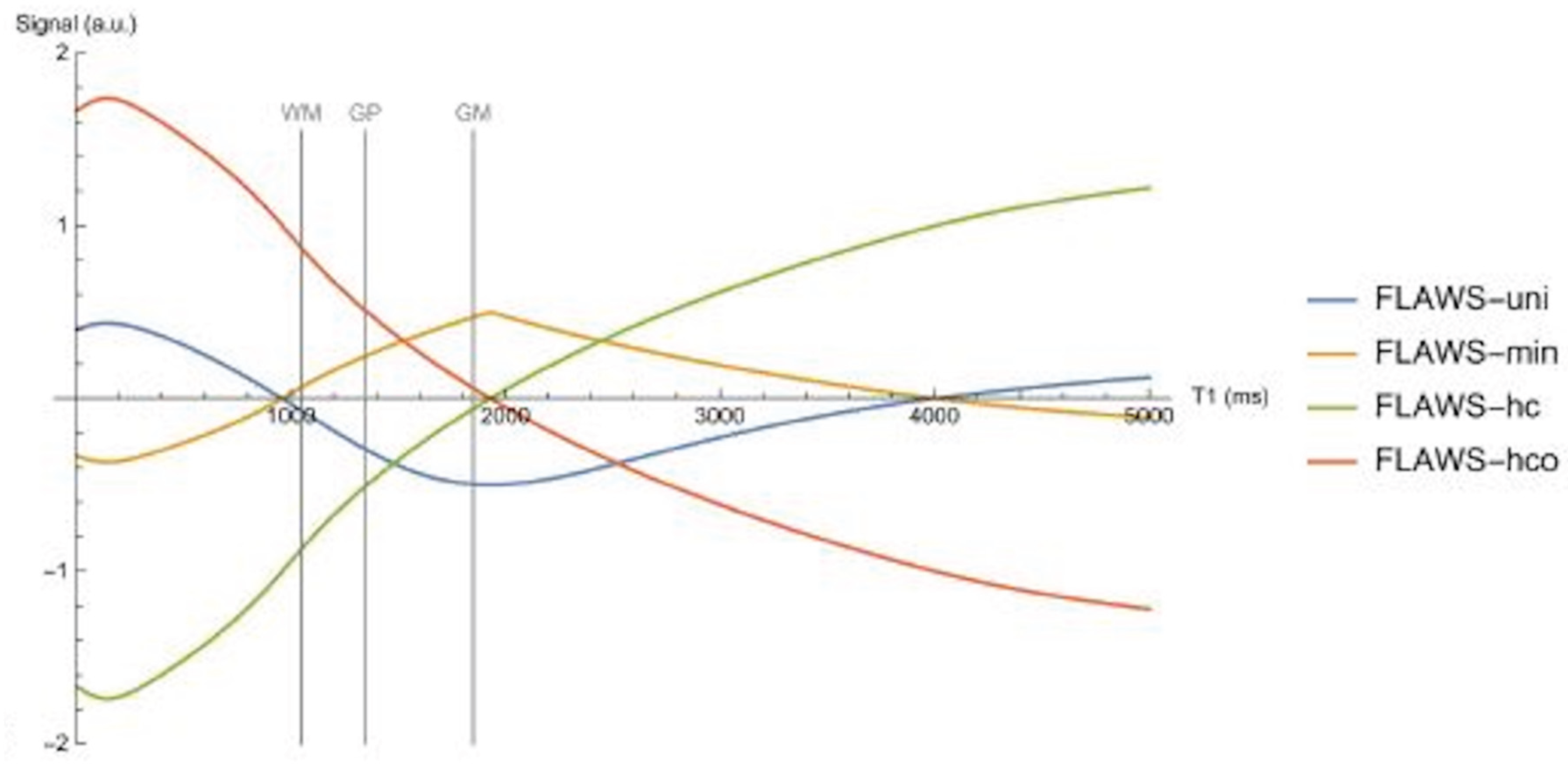
This sequence multiplies the signals of two IR sequences together and divides this by the sum of the squares of the signals from the two sequences. Complex multiplication is employed. Signal values vary between ± ½. It is a negative unipolar T1-filter for brain and has a moderate negative slope between white matter and gray matter with a shallower positive slope between gray matter and CSF (Figure 26, blue curve labelled FLAWS-uni which is identical with MP2RAGE). The sequence places white matter at the upper end of the display scale, gray matter at the lower end of the display scale and CSF at an intermediate level which is similar to the divided reverse SIR (drSIR) sequence but the reverse of the dSIR sequence.
Fluid and White Matter Suppression High Contrast (FLAWS-hc), FLAWS- High Contrast Opposite (FLAWS-hco) and FLAWS-Minimum (FLAWS-min) [23,24]
The FLAWS-hc and FLAWS-hco sequences have the same general mathematical form as the dSIR and drSIR sequences i.e. subtraction of two IR sequences divided by their sum i.e. , but differ in important ways: firstly, the TIs used are widely separated as opposed to dSIR and drSIR sequences where the TIs are usually narrowly separated in order to specifically target small differences or changes in T1 in tissues. Secondly, complex multiplication is used and the images are in phase-sensitive form not magnitude form. In Figure 26 the FLAWS-hc filter (green) has a positive slope over a very wide T1 domain and the FLAWS-hco filter (orange) has a negative slope over the same very wide Domain. The magnitude of the slopes of the two filters are generally greater than that of the FLAWS-min/MP2RAGE filter. The monotonic form of the FLAWS-hc and FLAWS-hco T1-filters is strikingly different from the bipolar form of dSIR and lSIR T1-filters which have well defined, sharp discontinuities at their null points due to the use of magnitude reconstruction. They also have steep positive slopes within narrow mDs rather than the broad lower magnitude slopes of the FLAWS-hc and FLAWS-hco filters over wide T1 Domains (Figure 26).
Figure 26.
Plots of signal vs T1 (T1-filters) for the FLAWS-uni/MP2RAGE (blue), FLAWS-min (yellow), FLAWS-hc (green) and FLAWS-hco (orange) T1-filters from Beaumont et al Fig 1B in reference [24]. The FLAWS-uni/MP2RAGE T1-filter (blue) is a negative unipolar filter for brain and CSF with a moderate negative slope between white matter (WM) and gray matter (GM), and a moderate positive slope between GM and CSF at 4000 ms. The CSF and WM signals are similar. The display range is from GM to WM. (GP is the globus pallidus). The FLAWS-min T1-filter (yellow) is a positive unipolar filter with a moderate positive slope from WM to beyond GM and a moderative negative slope from this point to CSF with CSF low signal. The display range is from WM and CSF to just higher than GM. The FLAWS-hc T1-filter (green) is monotonic for brain and CSF. It has a higher positive slope than the magnitude of the FLAWS-min/MP2RAGE slope from WM to GM and CSF has a very high signal. WM is at the lowest level on the display range and CSF is at the highest level. The FLAWS-hco T1-filter is monotonic with a higher size of slope than FLAWS-uni/MP2RAGE between WM and GM and a very low signal for CSF. The display range is from CSF to white matter. (Reproduced with permission: from Beaumont et al [24]).
The FLAWS-min filter is the lower signal from two IR T1-filters, one nulling white matter and the other nulling CSF. This is divided by the sum of the signals from the two filters and has a maximum value of a ½ and a minimum value of zero for the brain. It follows the shorter TI nulling IR filter in the lower part and the longer TI nulling IR filter in the higher part of the T1 Domain. It is a positive unipolar filter with the lowest signal nulling white matter, a peak at a T1 just greater than the T1 of gray matter, and CSF as zero signal (Figure 26). It has similarities to the narrow mD dSIR sequence but has a lower display range and a lower slope. Müller et al described a halo sign when imaging MS lesions in the cortex with the FLAWS-min sequence (Figure 5 in reference [25]). This is due to an increase in cortex T1 in lesions passing through the peak of the FLAWS-min filter into longer T1 regions. The slope of the T1-filter of the FLAWS-min sequence around its maximum value is relatively low and this may account for the greater width of the halo sign compared with the width of the bubble sign found with the narrow mD dSIR sequence when there is an increase in T1 through the peak of that sequence (e.g. Figure 16B). There are also high signal boundaries between ventricular white matter and CSF as well as between white matter and a periventricular lesion with the FLAWS-min sequence (in Figure 5, reference [25]) as expected from its T1-filter.
A similar pattern is seen in the leukocortical lesion shown in Figure 2B of reference [26] using T1w-FLAWS which is the same as FLAWS-min. However, the cortical lesion shown in the same figure imaged with T1w-FLAWS shows low contrast with the surrounding normal gray matter. Increased signal is seen at the boundary between gray matter and CSF. These features are consistent with Figure 26 (blue curve for FLAWS-min). FLAWS-min images do not show high signal between white matter and gray matter because the peak signal on the FLAWS-min T1-filter is not between these two tissues. If the second nulling TI (of CSF) is reduced, the FLAWS-min sequence becomes more like a narrow mD dSIR filter but with lower magnitude slopes.
In summary, the MP2RAGE and FLAWS T1-filters are unipolar or monotonic, not bipolar. They have fixed TIs and wide T1 Domains with lower slopes than narrow mD dSIR T1-bipolar filters in their mDs. The FLAWS-uni/MP2RAGE T1-filter has a moderate slope, reduced CSF signal and shows white and gray matter at the upper and lower ends of the display scale. FLAWS-hc has a higher slope than FLAWS-uni/MP2RAGE, with CSF very high signal and a wide display range from WM to CSF. FLAWS-hco also has a higher magnitude negative slope than FLAWS-uni/MP2RAGE with CSF very low signal and a wide display range from CSF to white matter. FLAWS-min has a positive T1-unipolar filter with a moderate slope and peak signal at a T1 just greater than that of gray matter. The T1-filters shown in Figure 26 provide a succinct and accessible way of comparing the signal levels and contrast performance of these sequences.
White Matter Nulled MP-RAGE [27] and Fast Gray Matter IR (FGATIR) [28]
These are single IR sequences that null white matter so that most of the remaining signal present in the brain is from gray matter. They have negative unipolar T1-filters. The slopes of their T1-filters are shown in Figure 6B and 6C when TI is chosen to null white matter. Small differences or changes in white matter from normal show much less contrast with white matter nulled MP-RAGE than with white matter nulled narrow mD dSIR sequences (Figure 6C). Boundaries between white matter and gray matter also show higher contrast with narrow mD sequences (Figure 7).
3D-Edge Enhancing Gradient Echo (3D-EDGE) [29] and EDGE-MP2RAGE [30] Sequences
The EDGE sequence has a single IR gradient echo with a negative unipolar T1-filter and a TI chosen to produce zero signal at the boundary between white and gray matter with equal signals in each tissue. It uses magnitude reconstruction. The boundary contains voxels with a mixture of the two tissues and a T1 between those of white and gray matter. It is of value in localising boundaries and diagnosing focal cortical dysplasia. EDGE-MP2RAGE acquires two separate images, the first of which is nulled in the same way as for the 3D-EDGE sequence. FGATIR, 3D-EDGE and EDGE-MP2RAGE images can be synthetically created from MP2RAGE derived T1 maps [31].
Funding
We have received support from the Fred Lewis Enterprise Foundation, the Hugh Green Foundation, Manaaki Moves, NZ P Pull, the JN & HB Williams Foundation, the Mangatawa Beale Williams Memorial Trust, Neurological Foundation, Trust Tairāwhiti, Friends of Mātai Blue Sky Fund, GE Healthcare, Mātai Ngā Māngai Maori, and Kānoa— Regional Economic Development & Investment Unit of New Zealand.
Informed consent
Written informed consent was obtained from all participants in this study.
Conflict of interest
GMB is a consultant to Magnetica, Brisbane, Australia. No other authors have any conflict of interest to disclose.
Ethical approval
All procedures performed in the studies involving human participants were in accordance with the ethical standards of the institutional and/or national research committee and with the 1964 Helsinki
Declaration and its later amendments or comparable ethical standards.
Abbreviations
| BLAIR | BipoLAr fIlteR, bipolar filter |
| cdSIR | composite divided Subtracted Inversion Recovery |
| clSIR | composite logarithmic then Subtracted Inversion Recovery |
| dSIR | divided Subtracted Inversion Recovery |
| hD | highest Domain |
| IR | Inversion Recovery |
| lSIR | logarithmic then Subtracted Inversion Recovery |
| mD | middle Domain |
| MP2RAGE | Magnetisation Prepared 2 Rapid Acquisition Gradient Echo |
| MT | Magnetisation Transfer |
| SIR | Subtracted Inversion Recovery |
| SOF | Signal from Other Filter |
| T1D | T1 Derivative |
| TP-bipolar filter | Tissue Property-bipolar filter |
| TP-filter | Tissue Property-filter |
| UHC | Ultra-High Contrast |
References
- Condron P, Cornfeld DM, Scadeng M, et al ( 2024) Ultra-high contrast MRI: the whiteout sign shown with divided subtracted inversion recovery (dSIR) sequences in post-insult leukoencephalopathy syndromes (PILS). Tomography 10(7):983-1013. [CrossRef]
- Ma Y-J, Shao H, Fan S, et al (2020) New options for increasing the sensitivity, specificity and scope of synergistic contrast magnetic resonance imaging (scMRI) using Multiplied, Added, Subtracted and/or FiTted (MASTIR) pulse sequences. Quant Imaging Med Surg 10(10):2030-2065. [CrossRef]
- Ma Y-J, Moazamian D, Port JD, et al (2023) Targeted magnetic resonance imaging (tMRI) of small changes in the T1 and spatial properties of normal and near normal appearing white and gray matter in disease of the brain using divided subtracted inversion recovery (dSIR) and divided reverse subtracted inversion recovery (drSIR) sequences. Quant Imaging Med Surg 13(10):7304-7337. [CrossRef]
- Newburn G, McGeown JP, Kwon EE, et al (2023) Targeted MRI (tMRI) of small increases in the T1 of normal appearing white matter in mild traumatic brain injury (mTBI) using a divided subtracted inversion recovery (dSIR) sequence. OBM Neurobiology 7(4):. [CrossRef]
- Ma Y-J, Moazamian D, Cornfeld DM, et al (2022) Improving the understanding and performance of clinical MRI using tissue property filters and the central contrast theorem, MASDIR pulse sequences and synergistic contrast MRI. Quant Imaging Med Surg 12(9):4658-4690.
- Cornfeld D, Condron P, Newburn G, et al (2024) Ultra-high contrast MRI: Using divided subtracted inversion recovery (dSIR) and divided echo subtraction (dES) sequences to study the brain and musculoskeletal system. Bioengineering 11:441. [CrossRef]
- Newburn G, Condron P, Kwon EE, et al (2024) Diagnosis of delayed post-hypoxic leukoencephalopathy (Grinker's myelinopathy) with MRI using divided subtracted inversion recovery (dSIR) sequences: time for reappraisal of the syndrome? Diagnostics 14(4):418. [CrossRef]
- Yokoo T, Bae WC, Hamilton G, et al (2010) A quantitative approach to sequence and image weighting. J Comput Assist Tomogr 34(3):317-331.
- Young IR, Szeverenyi NM, Du J, Bydder GM (2020) Pulse sequences as tissue property filters (TP-filters): a way of understanding the signal, contrast and weighting of magnetic resonance images. Quant Imaging Med Surg 10(5):1080-1120.
- Bydder, M., Cornfeld, D.M., Melzer, T.R. et al (2025) Log subtracted inversion recovery. Magn Reson Imaging 117:110328.
- Ugurbil K (2014) Magnetic resonance imaging at ultrahigh fields. IEE Trans Biomed Eng 61:1364-1379.
- Feinberg DA, Beckett AJS, Vu AT, et al (2023) Next-generation MRI scanner designed for ultra-high-resolution human brain imaging at 7 Tesla. Nat Methods 20:2048-2057. [CrossRef]
- Bydder M, Condron P, Cornfeld DM, et al (2024) Validation of an ultra-high contrast divided subtracted inversion recovery technique using a standard T1 phantom. NMR Biomed 2024;e5269.
- Losa L, Peruzzo D, Galbiati S, Locatelli F, Agarwal N (2024) Enhancing T1 signal of normal-appearing white matter with divided subtracted inversion recovery: a pilot study in mild traumatic brain injury. NMR Biomed 37(10):e5175. [CrossRef]
- Hajnal JV, Baudouin CJ, Oatridge A, Young IR, Bydder GM (1992) Design and implementation of magnetisation transfer pulse sequences for clinical use. J Comput Assist Tomogr 16(1):7-18.
- Nürnberger L, Gracien R-M, Hok P, et al (2017) Longitudinal changes of cortical microstructure in Parkinson's disease assessed with T1 relaxometry. NeuroImage Clinical 13:405-414.
- Roeben B, Zeltner L, Hagberg GE, Scheffler K, Schols L, Bender B (2023) Susceptibility-weighted imaging reveals subcortical iron deposition in PLA2G6-associated neurodegeneration: the "Double Cortex Sign". Mov Disord 38(5):904-906.
- Mueller SG (2024) 7T MP2RAGE for cortical myelin segmentation: impact of aging. PLoS One 19(4):e0299670.
- Bydder GM, Young IR (1985) MR imaging: clinical use of the inversion recovery sequence. J Comput Assist Tomogr 9(4):659-675.
- Redpath TW, Smith FW (1994) Technical note: use of a double inversion recovery pulse sequence to image selectively grey or white brain matter. Br J Radiol 67(804):1258-1263.
- Tillema J-M, Weigand SD, Dayan M, et al (2018) Dark rims: novel sequence enhances diagnostic specificity in multiple sclerosis. AJNR Am J Neuroradiol 39(6):1052-1058. [CrossRef]
- Marques JP, Kober T, Krueger G, van der Zwaag W, Van de Moortele P-F, Gruetter R (2010) MP2RAGE, a self bias-field corrected sequence for improved segmentation and T1-mapping at high field. Neuroimage 49(2):1271-1281. [CrossRef]
- Beaumont J, Saint-Jalmes H, Acosta O, et al (2019) Multi T1-weighted contrast MRI with fluid and white matter suppression at 1.5T. Magn Reson Imaging 63:217-225.
- Beaumont J, Gambarota G, Saint-Jalmes H, et al (2021) High-resolution multi-T1-weighted contrast and T1 mapping with low B1 sensitivity using the fluid and white matter suppression (FLAWS) sequence at 7T. Magn Reson Med 85(3):1364-1378.
- Müller J, La Rosa F, Beaumont J, et al (2022) Fluid and white matter suppression. New sensitive 3T magnetic resonance imaging contrasts for cortical lesion detection in multiple sclerosis. Invest Radiol 57(9):592-600.
- Durozard P, Maarouf A, Zaaraoui W, et al (2024) Cortical lesions as an early hallmark of Multiple Sclerosis: visualization by 7T MRI. Invest Radiol 59(11):747-753. [CrossRef]
- Saranathan M, Tourdias T, Bayram E, Ghanouni P, Rutt BK (2015) Optimization of white-matter-nulled magnetization prepared rapid gradient echo (MP-RAGE) imaging. Magn Reson Med 73(5):1786-1794. [CrossRef]
- Grewal SS, Middlebrooks EH, Kaufmann TJ, et al (2018) Fast gray matter acquisition T1 inversion recovery MRI to delineate the mammillothalamic tract for preoperative direct targeting of the anterior nucleus of the thalamus for deep brain stimulation in epilepsy. Neurosurg Focus 45(2):E6. [CrossRef]
- Middlebrooks EH, Lin C, Westerhold E, et al (2020) Improved detection of focal cortical dysplasia using a novel 3D imaging sequence: Edge-Enhancing Gradient Echo (3D-EDGE) MRI. NeuroImage 28:102449. [CrossRef]
- Tao S, Zhou E, Greco V, et al (2023) Edge-Enhancing Gradient-Echo MP2RAGE for clinical epilepsy imaging at 7T. AJNR Am J Neuroradiol 44(3):268-270.
- Middlebrooks EH, Tao S, Zhou X, et al (2023) Synthetic inversion image generation using MP2RAGE T1 mapping for surgical targeting in deep brain stimulation and lesioning. Stereotact Funct Neurosurg 101:326-331. [CrossRef]
Figure 1.
Positionally matched images of the brain in a 24-year-old male patient with mTBI (A and C) and a normal control (B). (A) is a T2-FLAIR image in the patient which shows no abnormality. (B) is a narrow mD dSIR image of the brain in the normal control. The white matter in the central region of this image has a normal low signal (dark) appearance (arrows). (C) is a narrow mD dSIR image performed in the patient with the same sequence as in the control. This image shows all the patient's white matter with abnormal high signal (light) (arrows) rather than the normal low signal (dark) appearance in the control (arrows) (B). There is a night and day difference in signal between normal and abnormal white matter in (B) and (C). High signal boundaries are seen between normal white matter and normal gray matter in (B). These are less obvious in (C) because of the high signal in the abnormal white matter.
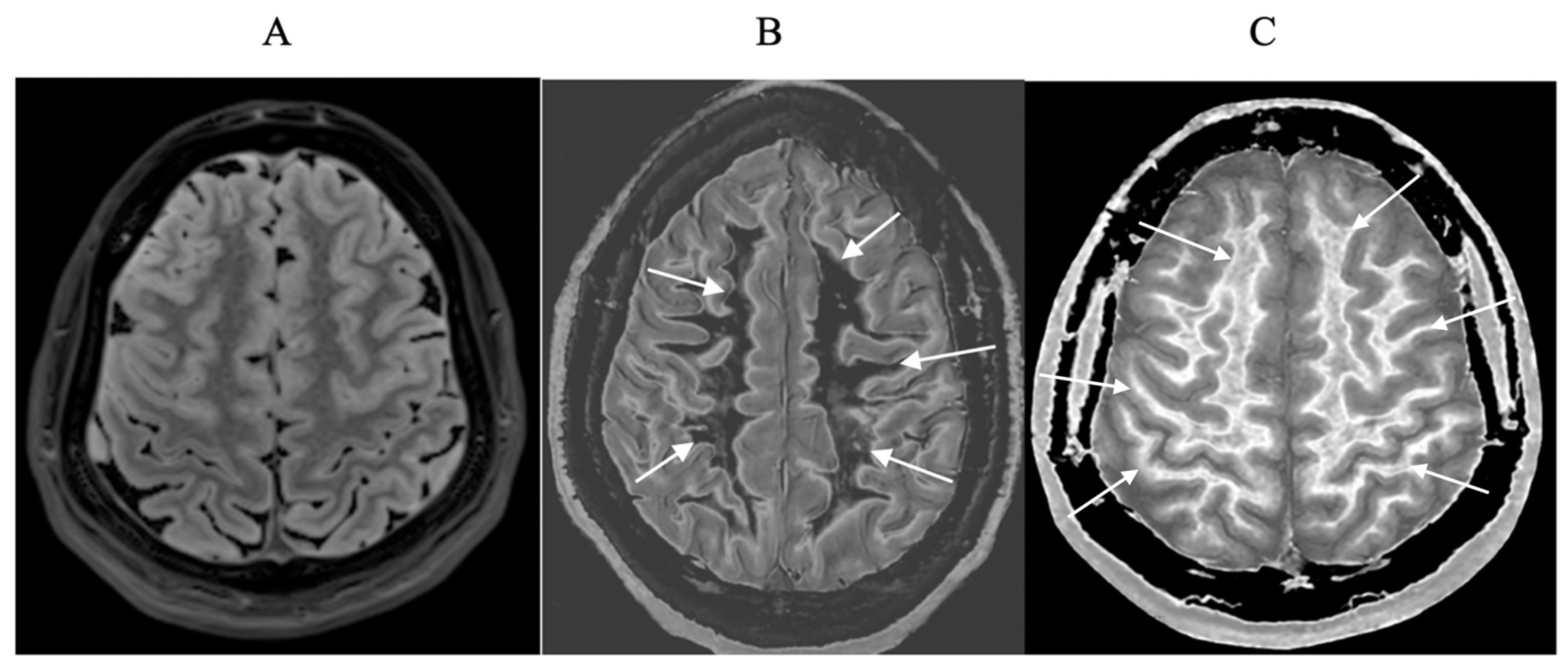
Figure 2.
Plot of MZ/MXY against time for a T2-weighted version of the SE sequence for two tissues P (with a shorter T1 and T2) and Q (with a longer T1 and T2). Overall T1 and T2 dependent contrast between P and Q is shown with the positive blue arrow on the right.
Figure 2.
Plot of MZ/MXY against time for a T2-weighted version of the SE sequence for two tissues P (with a shorter T1 and T2) and Q (with a longer T1 and T2). Overall T1 and T2 dependent contrast between P and Q is shown with the positive blue arrow on the right.
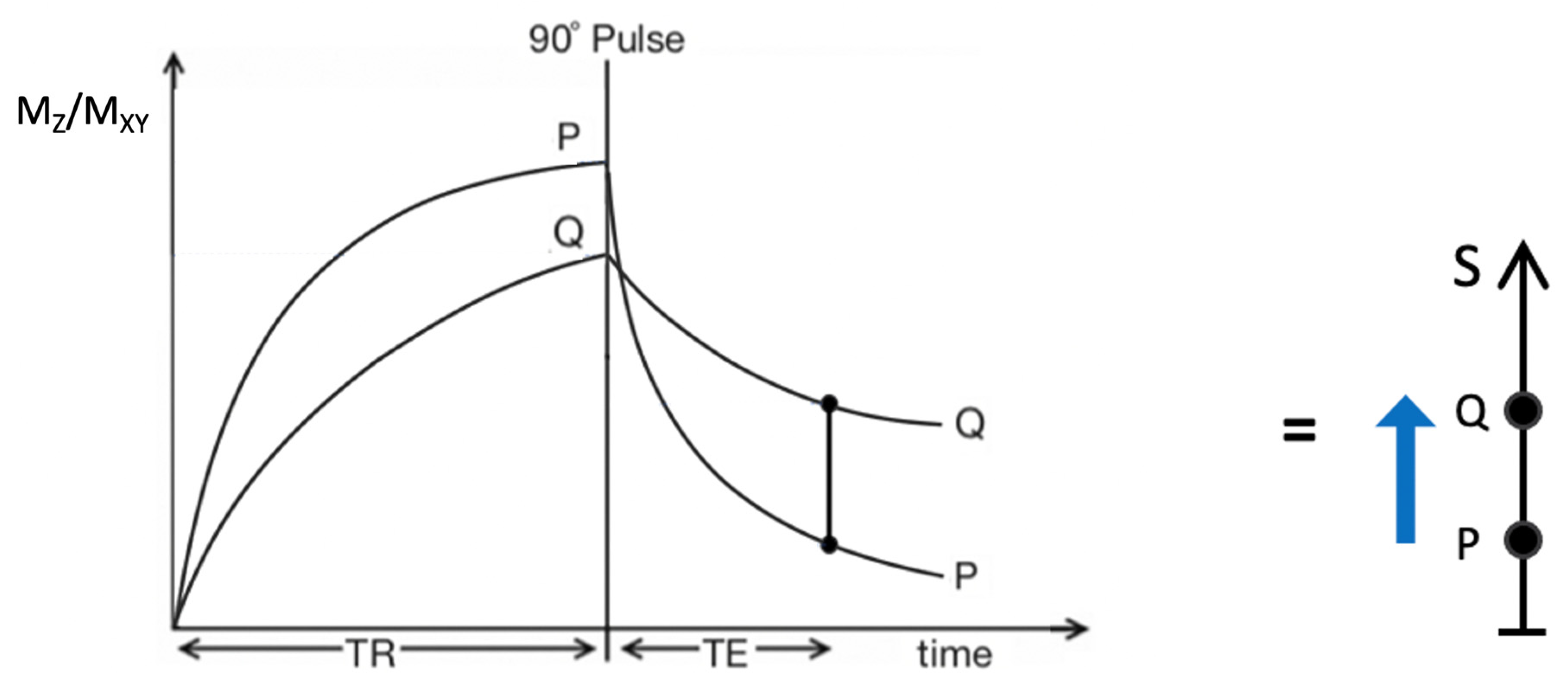
Figure 3.
IR T1-filters with plots of signal ST1 against T1 in phase-sensitive (A) and magnitude forms (B). (A) is a low pass filter and (B) is a negative unipolar filter. (A) shows both positive and negative values for ST1 whereas (B) shows negative values "reflected" across the X axis so they become positive. The maximum size of the slopes of the two T1-filters which are tangential to the slope are shown as red lines. The slopes are negative in both cases. .
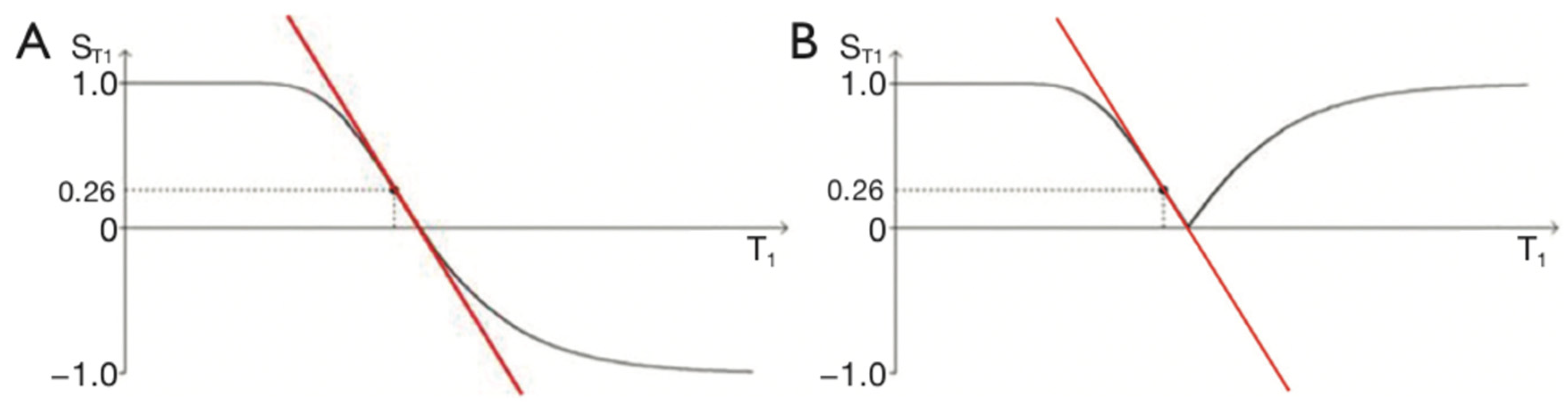
Figure 4.
The long TR IR sequence. Negative T1-unipolar filters for short TIs (A, left), intermediate TIi (B, centre) and long TIl (C, right) including white (W) and gray (G) matter. Signal ST1 is plotted against T1 in each case (black curves). The positions of W and G are the same at each of the three TIs. TI is increased from TIs (left) to TIi (centre) and increased further to TIl (right). In (A), (B) and (C), the increase in T1 from W to G (horizontal positive green arrows) is multiplied by the relevant slopes of the filters (red lines) to produce contrast. This is moderately positive, strongly negative, and mildly negative contrast in (A), (B) and (C) respectively (vertical blue arrows).
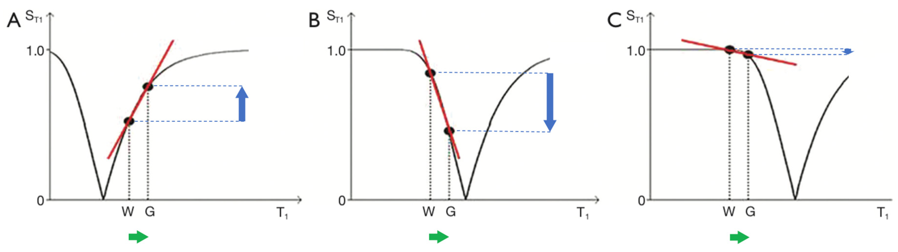
Figure 5.
Unipolar IR (A), subtracted IR (SIR) (B) and Added IR (AIR) (C) T1-filters. T1 is shown along the X axes in ms. (A) shows a TIs T1-unipolar filter (pink) and a TIi T1-unipolar filter (blue), (B) shows the subtraction (STIs - STIi) IR or SIR T1-bipolar filter, and (C) shows the addition (STIs + STIi) IR or AIR T1- filter. The vertical lines divide the X axes into lowest, middle and highest Domains (lD, mD and hD). The mD contains T1 values between the vertical dashed lines. In (B) the slope of the curve of the SIR T1-filter in the mD is about double that of the STIs T1-filter (pink in [A]). In (C) the signal at T1=0 is doubled to 2.0, and the signal in the mD is reduced to about 0.20 in the nearly linear, slightly downward sloping central part of the AIR T1-filter (i.e., in the mD).
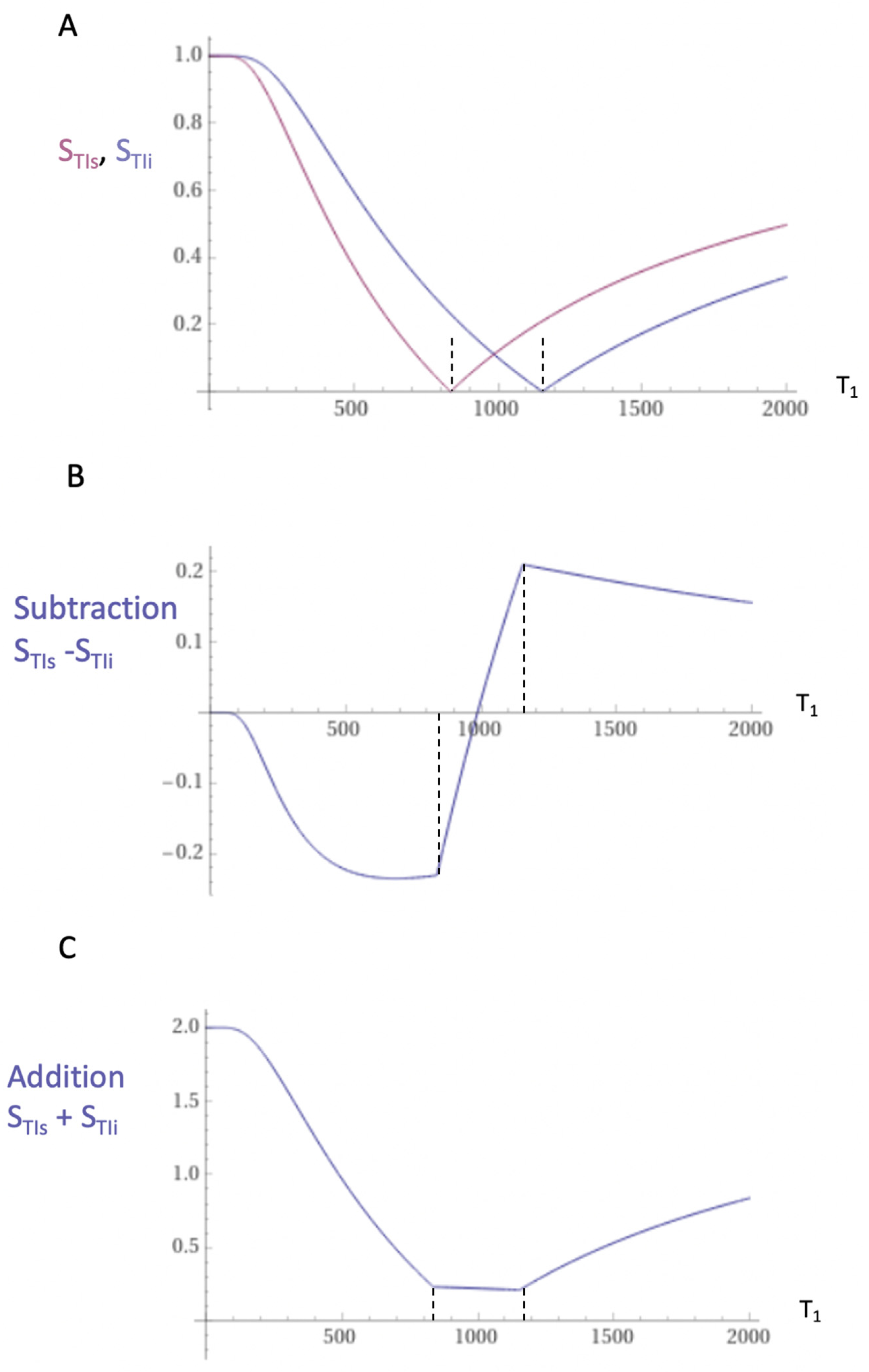
Figure 6.
Figure 6A shows division of the SIR T1-bipolar filter in Figure 5B by the addition T1-filter AIR in Figure 5C to give the dSIR T1-bipolar filter. T1 is shown along the X axis in ms. Figure 6B shows comparison of the conventional IR STIs T1-unipolar filter (pink) with the SIR T1-bipolar filter (blue) for a small increase in T1 (horizontal positive green arrow, ΔT1). Figure 6C is a comparison of the STIs T1-unipolar filter (pink) with the dSIR T1-bipolar filter (blue) for the same small increase in T1. In 6B the contrast produced by the SIR T1-bipolar filter is about twice that produced by the IR T1-unipolar filter (blue and pink arrows). In 6C the contrast produced by the dSIR T1-bipolar filter is about ten times greater than that produced by the IR T1-unipolar filter (blue and pink arrows). The display gray scale has no negative values so white matter appears on it as zero signal (black) at the lowest part of the display scale when using both the T1-filters shown in each of Figure 6B and Figure 6C.
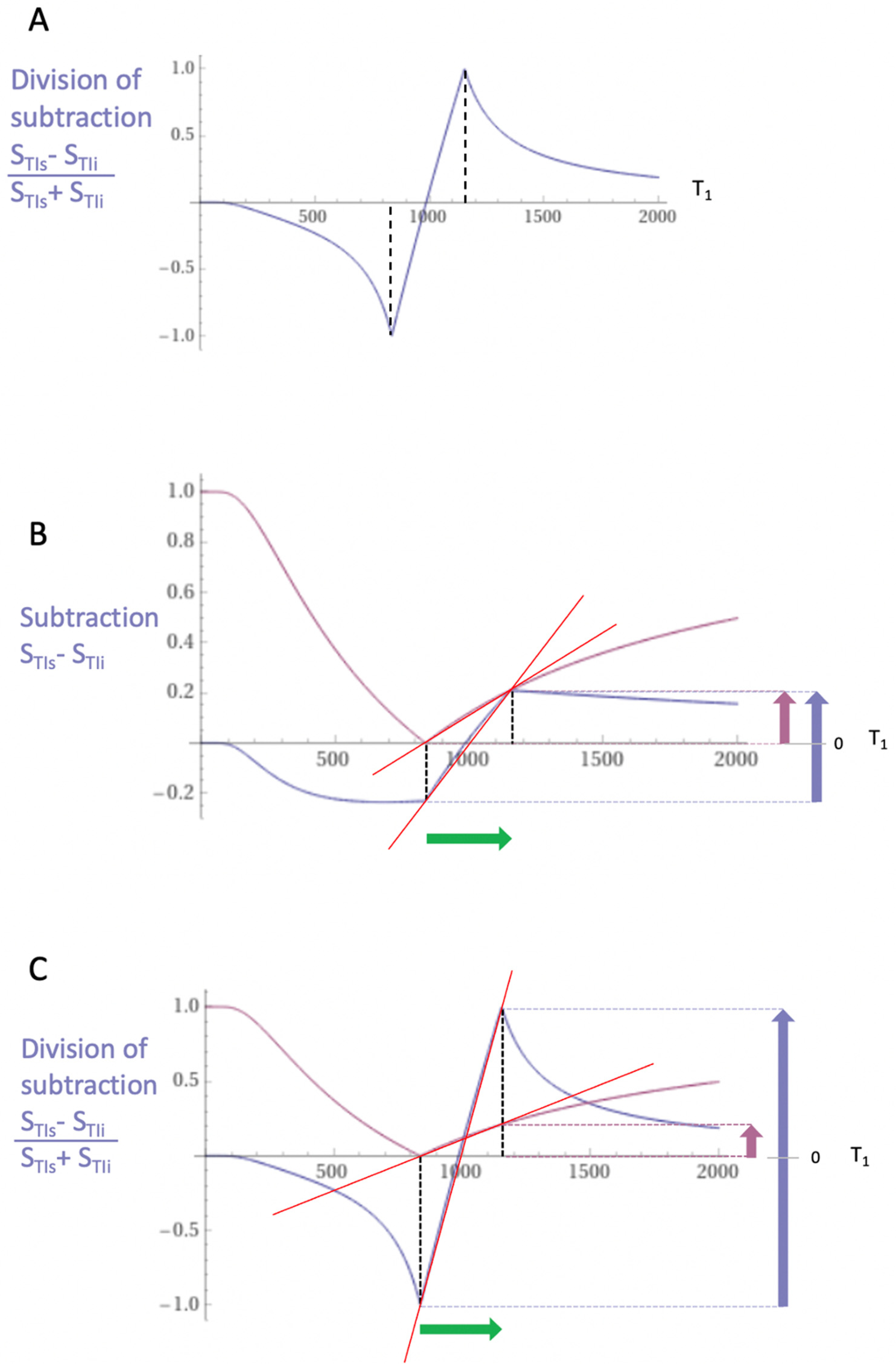
Figure 7.
Boundaries. This image shows a narrow mD dSIR T1-bipolar filter with a mD extending from white matter (W) to a T1W,G between the TIs of W and gray matter (G) (blue curve) as well as a white matter nulled conventional IR T1-unipolar filter e.g., MP-RAGE (pink curve). The X axis is shown in ms. The contrast produced from the difference in signal between W and G by the T1-unipolar filter is (SG minus SW, pink curve) and is shown by the vertical pink arrow. With the T1-bipolar filter (blue curve) there is a partial volume effect between W and G producing a T1W,G between the T1s of W and G which results in the high signal, SW,G shown on the T1-bipolar filter (blue curve). The contrast between this high signal and white matter is the difference (SW,G minus SW, in blue) and is shown by the vertical blue arrow. The contrast produced by the T1-bipolar filter at the boundary between W and G is far greater than that produced at the boundary between W and G by the T1-unipolar filter.
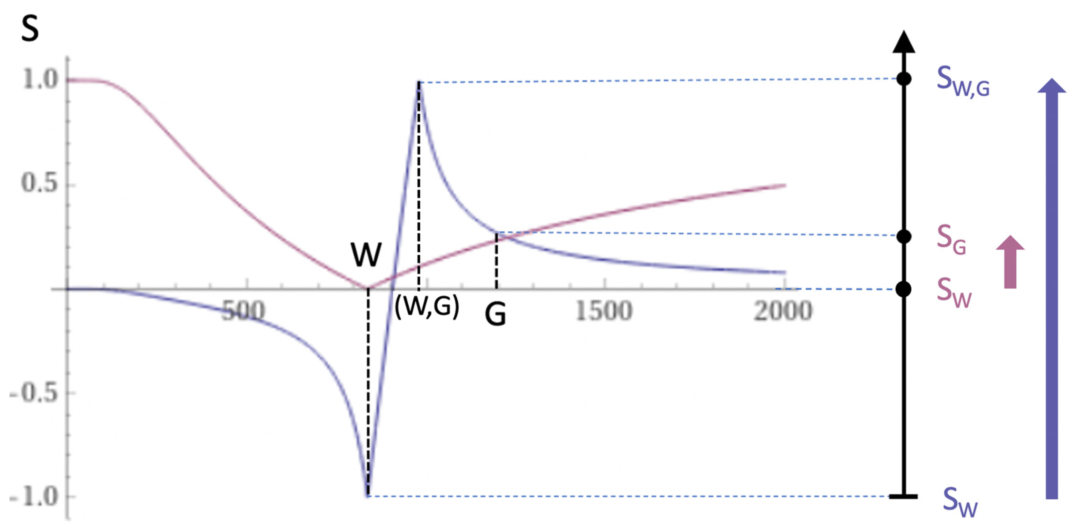
Figure 8.
Plots of ln STIs (TIs = 350 ms) vs T1 (pink), and ln STIi (TIi = 500 ms) vs T1 (blue). The plots have a negative unipolar form with steeply sloping signal gradients around their negative poles. The pink and blue ln STIs and ln STIi curves are steeper than the corresponding magnitude curves shown in Figure 5A. The lSIR filter SlSIR = ½(ln STIs - ln STIi) reverses the sign of the STIi filter so it becomes positive as seen in the following figure (Figure 9) (orange curve).
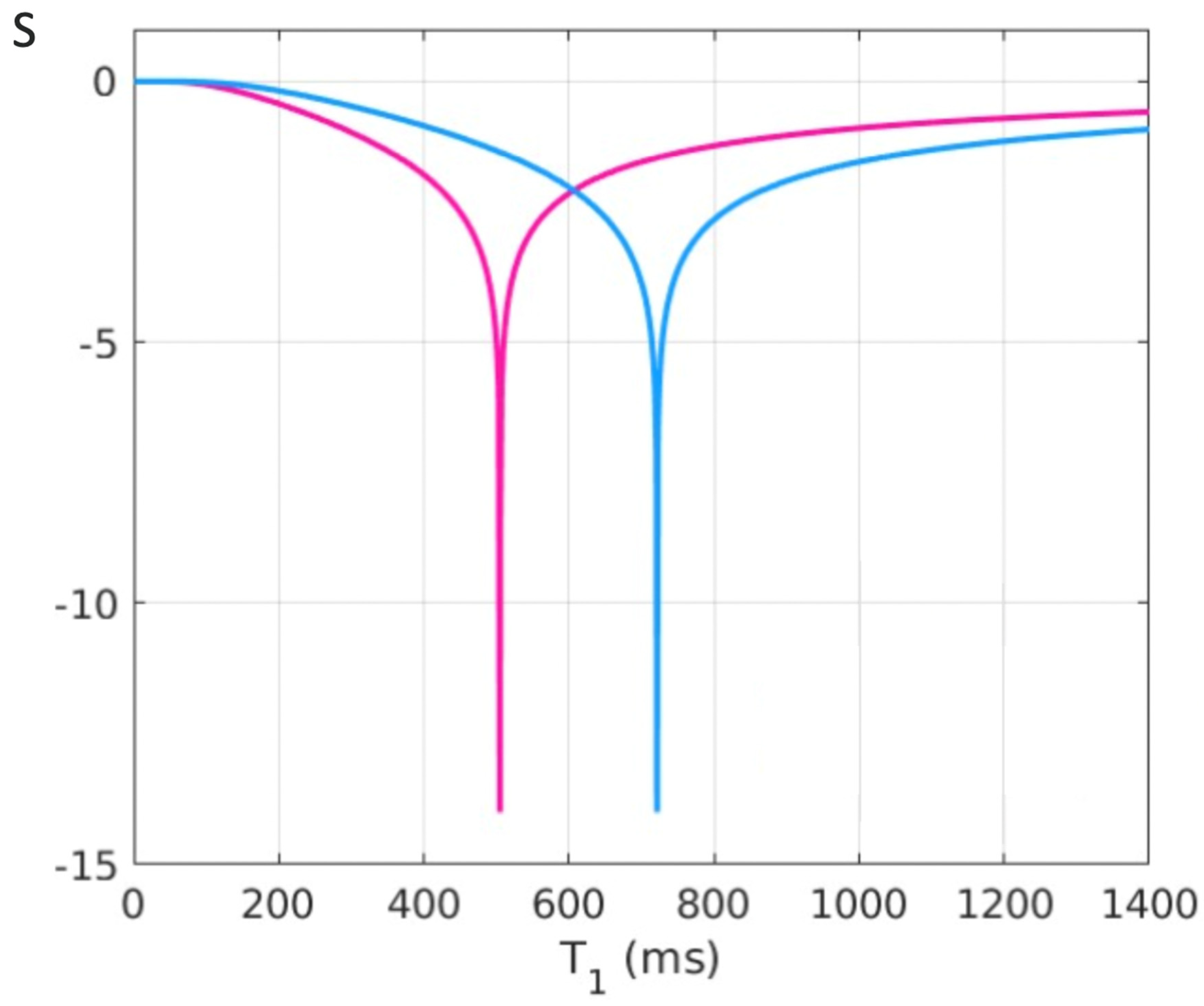
Figure 9.
Plot of signal vs T1 in ms for a dSIR T1-bipolar filter (blue curve) and the corresponding lSIR T1-bipolar filter with the same null points (orange curve) (TIs = 350 ms and TIi = 500 ms, ΔTI = 150 ms). The dSIR filter shows the usual pattern with maximum values of ±1. It has an essentially constant slope in the mD. The lSIR filter has similar values to the dSIR filter in the regions of lowest and highest values of T1 as well as in the centre of the mD. However around the lower and upper T1 nulling values it has much steeper slopes and proceeds asymptotically to minus and plus infinity respectively (values of S along the Y axis in the range of ± 2 are shown). From a practical point of view, the contrast for very small differences or changes in T1 is 2-3 times greater with the lSIR filter compared with the corresponding dSIR filter. For the same difference in T1 in the regions close to the null points the lSIR filter is steeper than the dSIR filter. This results in greater contrast and spatial resolution.
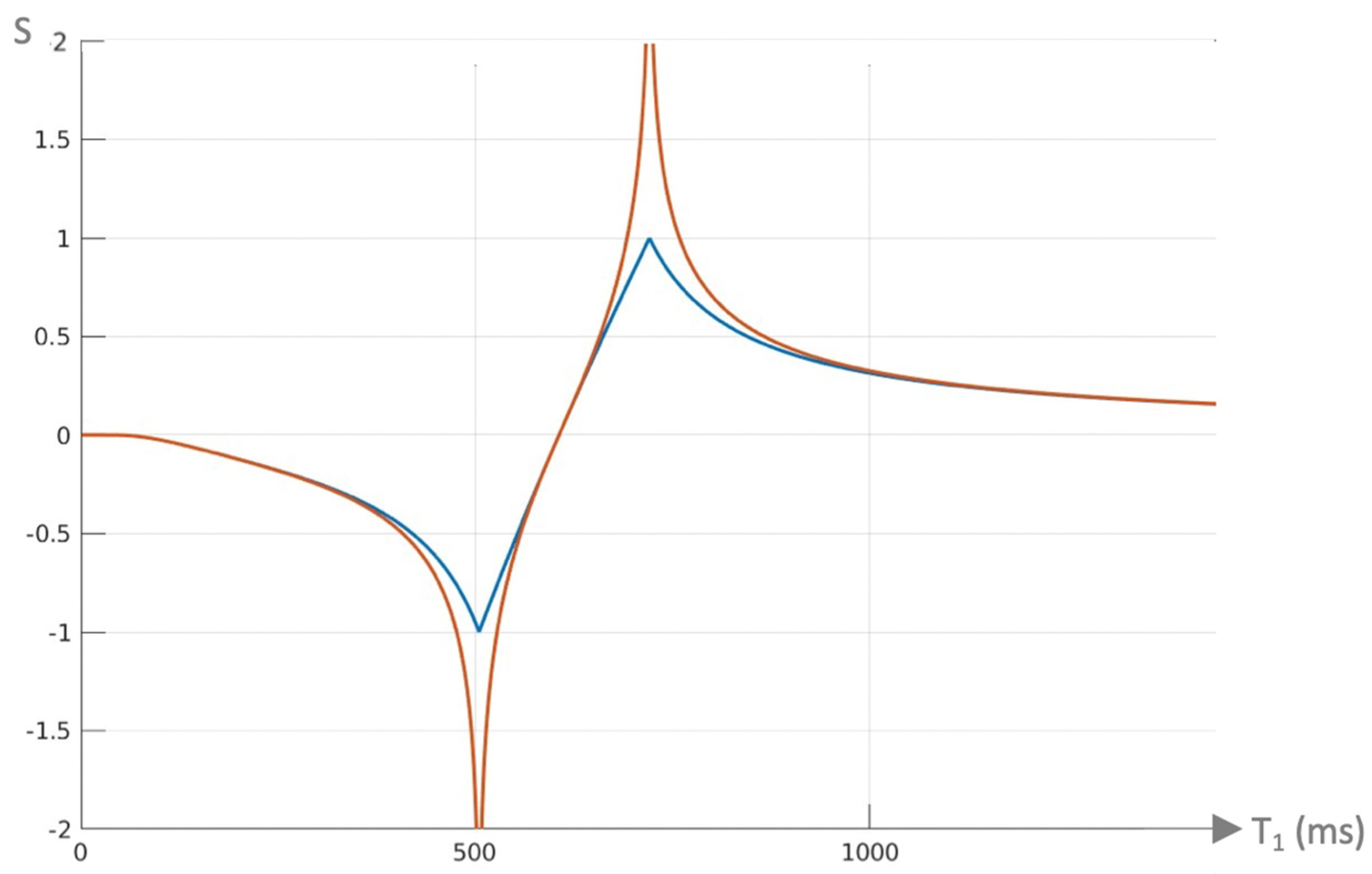
Figure 10.
Composite dSIR filters (cdSIRs with TIs = 350 ms and TIi = 500 ms). Attenuated first IR T1-filter (TIs) in (A) and attenuated second IR T1-filter (TIi) in (B). (A) shows the conventional T1-bipolar filter (blue) with SOF = 1, an attenuated first TIs filter (SOF = 0.5) (red) and a further attenuated first TIs filter (SOF = 0.25) (yellow). In (A), as SOF is decreased to 0.5 and 0.25 the filters around the first negative pole become wider and are positioned outside the blue filter. The attenuated filters around the second positive pole show higher contrast and become narrower. They are located inside the blue filter. (B) shows the conventional T1-bipolar filter (blue) with SOF = 1, and attenuated second TIi filter SOF = 0.5 (red) and a more attenuated second TIs filter (SOF = 0.25) (yellow). As SOF is decreased, the filters around the first negative pole become narrower and show higher contrast. They are positioned within the blue filter. The attenuated filters around the second positive pole become wider and show lower contrast. They are positioned outside of the blue filter. For T2, a short T2 increases attenuation relative to a longer T2 and this corresponds to the narrower and sharper peak with greater negative contrast and spatial resolution of the contrast (A).
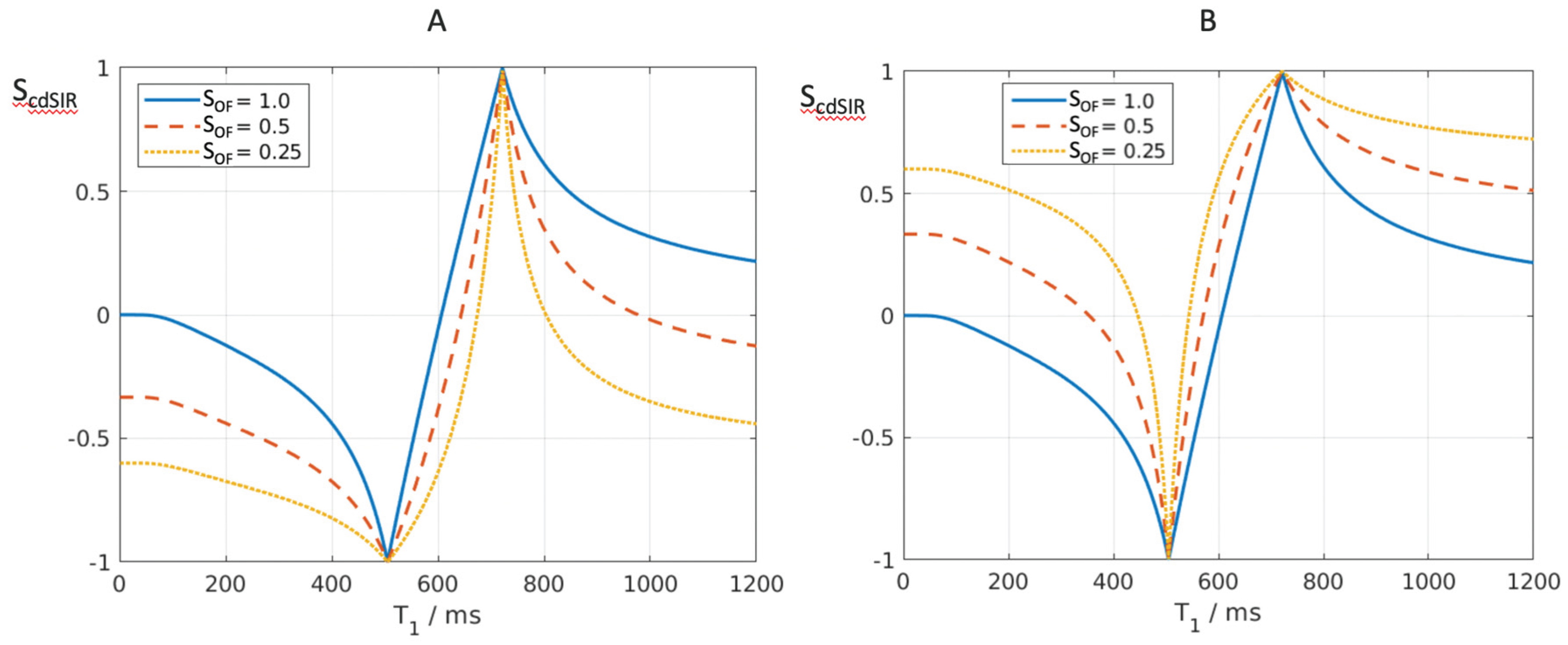
Figure 11.
Comparison of conventional windowing (A and B) and a dSIR T1-bipolar filter (C). (A) plots the display signal SD against image signal S for two tissues P and Q over the full image gray scale range shown along the Y axis. There is a linear relationship between SD and S over the full gray scale range. In (B) the image is narrowly windowed to place the signals from P and Q at the lower and upper ends of the SD range shown on the Y axis. The contrast between P and Q (difference in signal level shown on the Y axis) is increased in (B) compared with (A). In (B) signal values less than P on the X axis are all shown at the lowest signal level on the Y axis, and signal values along the X axis greater than Q are all shown at the highest signal level on the Y axis (horizontal lines). In these regions, voxels have the same signals and show no contrast between them. They form isointense blocks and anatomical detail is lost within the blocks. (C) plots signal against T1 using a dSIR T1-bipolar filter. Contrast between P and Q is high in the mD as in (B). Values of T1 less than P and greater than Q do not form plateaux as in (B) but follow the T1-bipolar filter in the lD and hD. There are therefore differences in signal between voxels so contrast is maintained and anatomical detail is preserved outside of the mD bounded by P and Q.
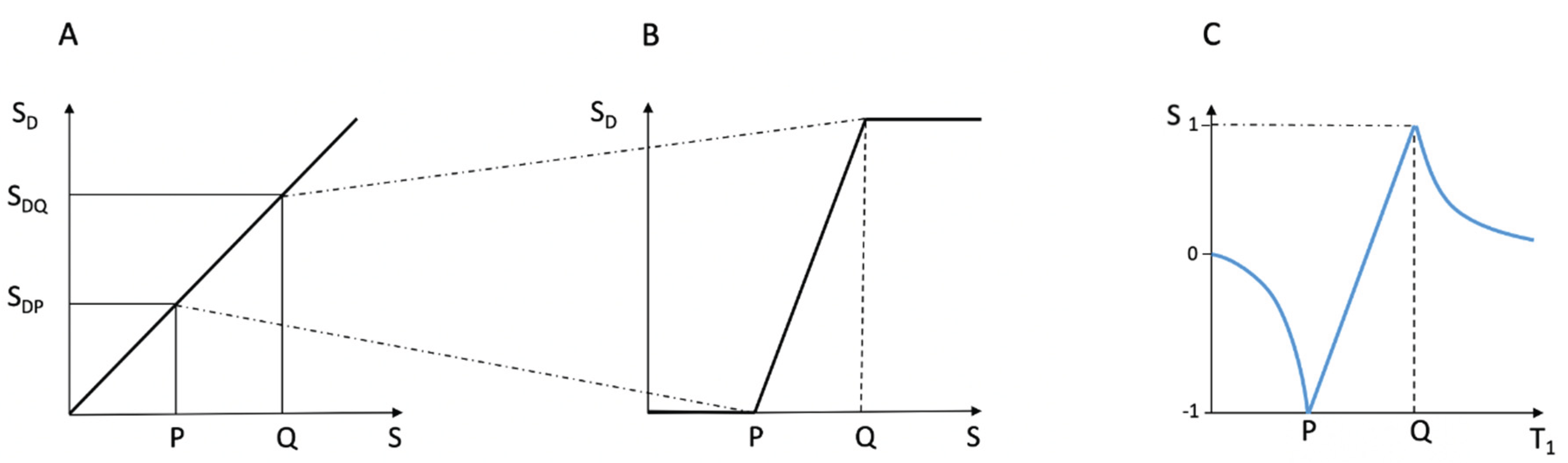
Figure 12.
18-year-old patient with mTBI 21h (A) and 64h (B) post injury imaged with the same narrow mD dSIR sequence. In (A) the patient shows a whiteout sign (grade 4 out of 5) with high signal in most of the white matter in the cerebral hemispheres except for the anterior and posterior central corpus callosum. The posterior limb of the internal capsule is high signal. The thalami show low internal contrast from medial to lateral (arrows on lateral margins of the thalami). There is also low external contrast between the lateral margins of the thalami and the adjacent posterior limbs of the internal capsule. On the follow up examination at 64h (B) the whiteout sign has resolved and there is low signal in the white matter including the posterior limbs of the internal capsule (except for the corticospinal tracts). The thalami now show high internal contrast from medial to lateral (arrows on lateral margins of the thalamus) which is the normal appearance at this age. There is now also very high external contrast between the lateral margin of the thalamus and the adjacent posterior limb of the internal capsule. Image (A) shows the grayout sign which is a reduction in the high contrast between the medial and lateral gray matter of the thalamus. The high contrast is restored in (B). No abnormality was seen on the corresponding T2-FLAIR images obtained at both time points.
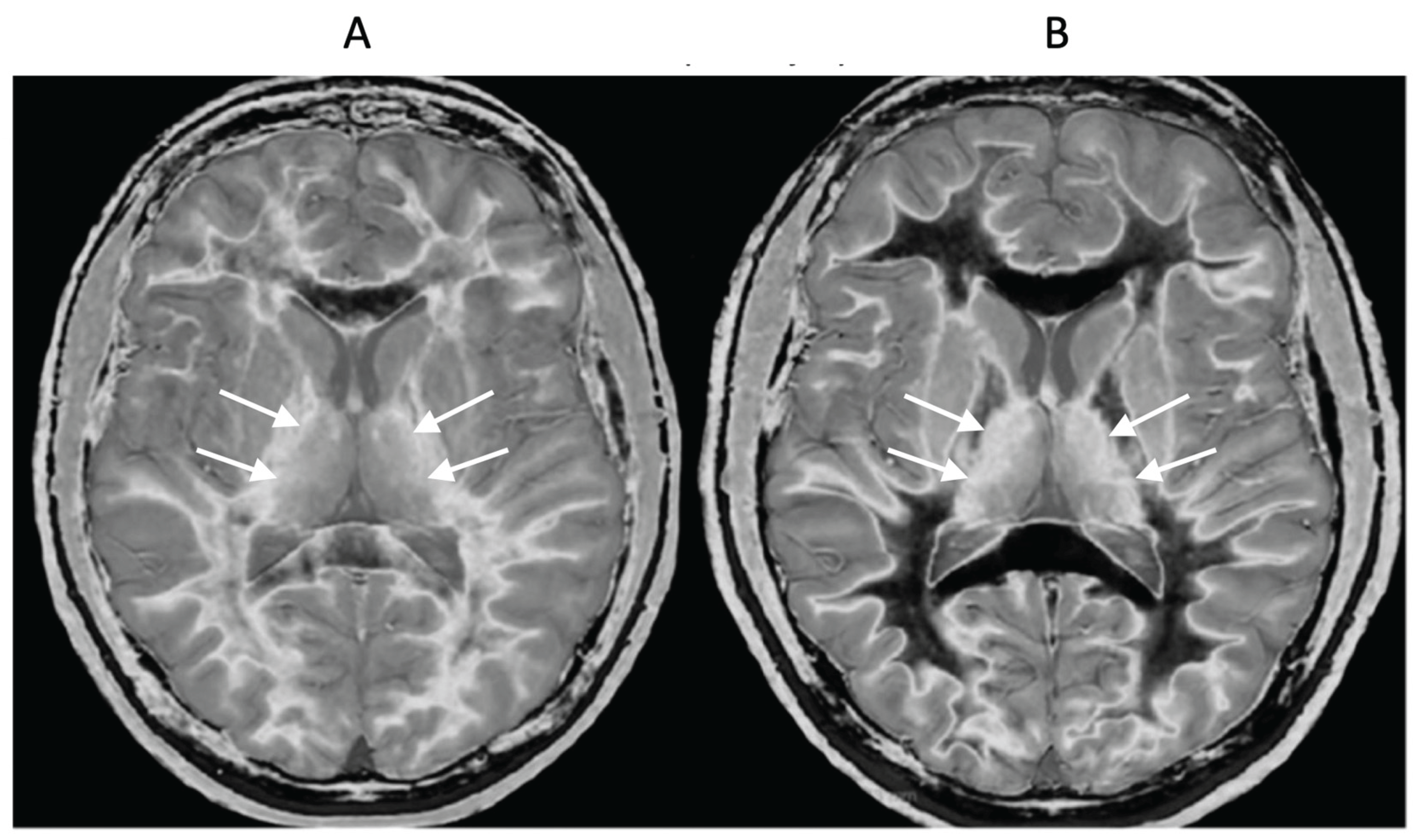
Figure 13.
Normal control (A) and patient with mTBI (B) showing a whiteout sign and grayout signs (narrow mD dSIR images). The normal control shows the heads of the caudate nuclei with higher signal than the adjacent CSF. Contrast is also seen between the cortex and CSF. In (B), the patient shows a whiteout sign. There are grayout signs in the thalami and putamina. In addition, contrast between the heads of the caudate nuclei and CSF is lost and there is little or no contrast between cortex and CSF which are isointense. These are also grayout signs. No abnormality was seen on the T2-FLAIR images in the normal control or patient.
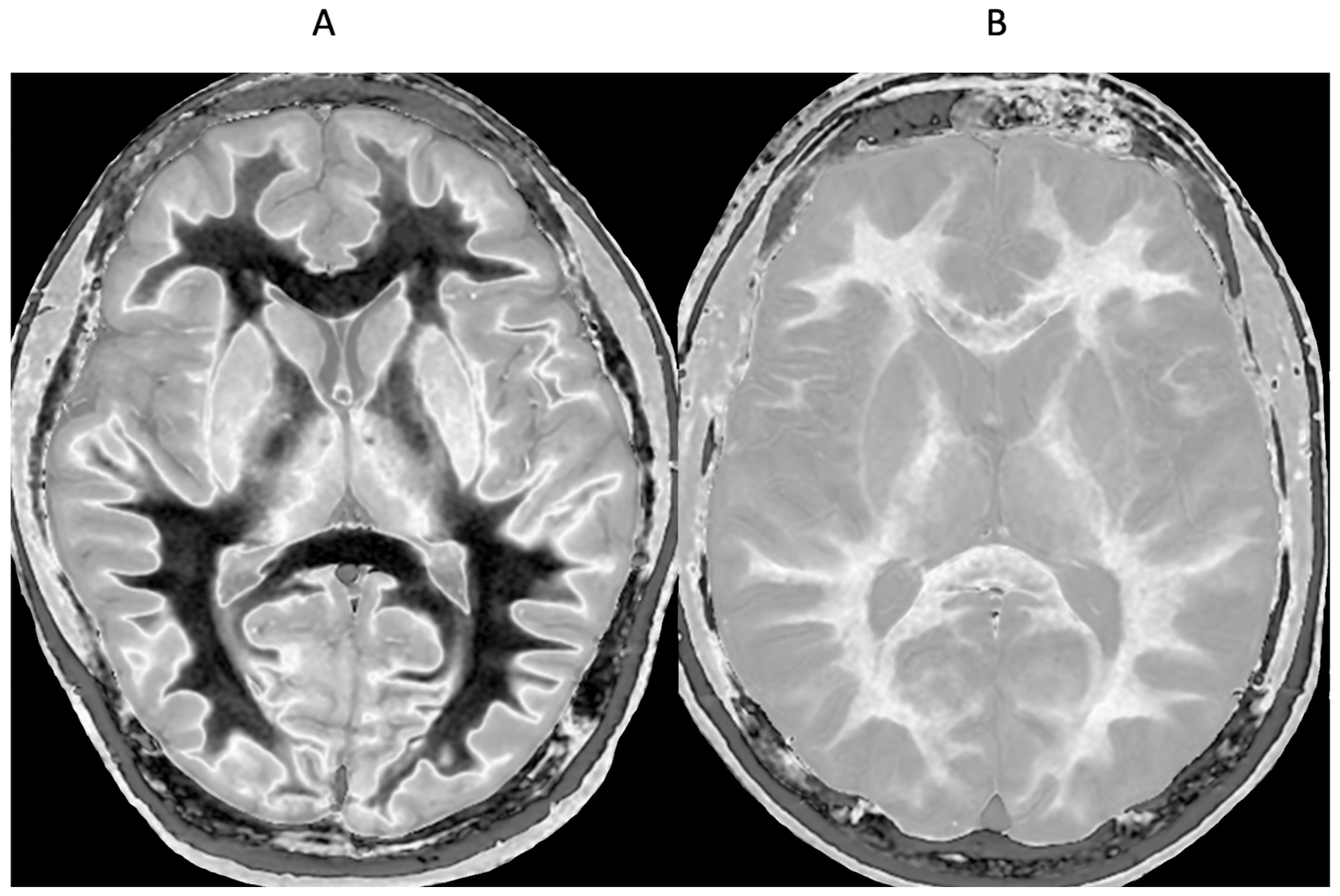
Figure 14.
Red nuclei in an 18-year-old normal control (A) and an 18-year-old male patient with mTBI (B). 2D narrow mD dSIR images. In (A) the normal control shows low signal in the white matter of the cerebral hemisphere, cortical spinal tracts and the ascending sensory tracts. The red nuclei (arrows) have an intermediate mid-gray signal. In (B) the patient shows high signal in the cerebral white matter, the corticospinal tracts and the ascending sensory tracts (whiteout sign, grade 4 out of 5). In addition, the red nuclei are higher signal than in (A) (arrows). No abnormality was seen on the T2-FLAIR images in the normal control or patient.
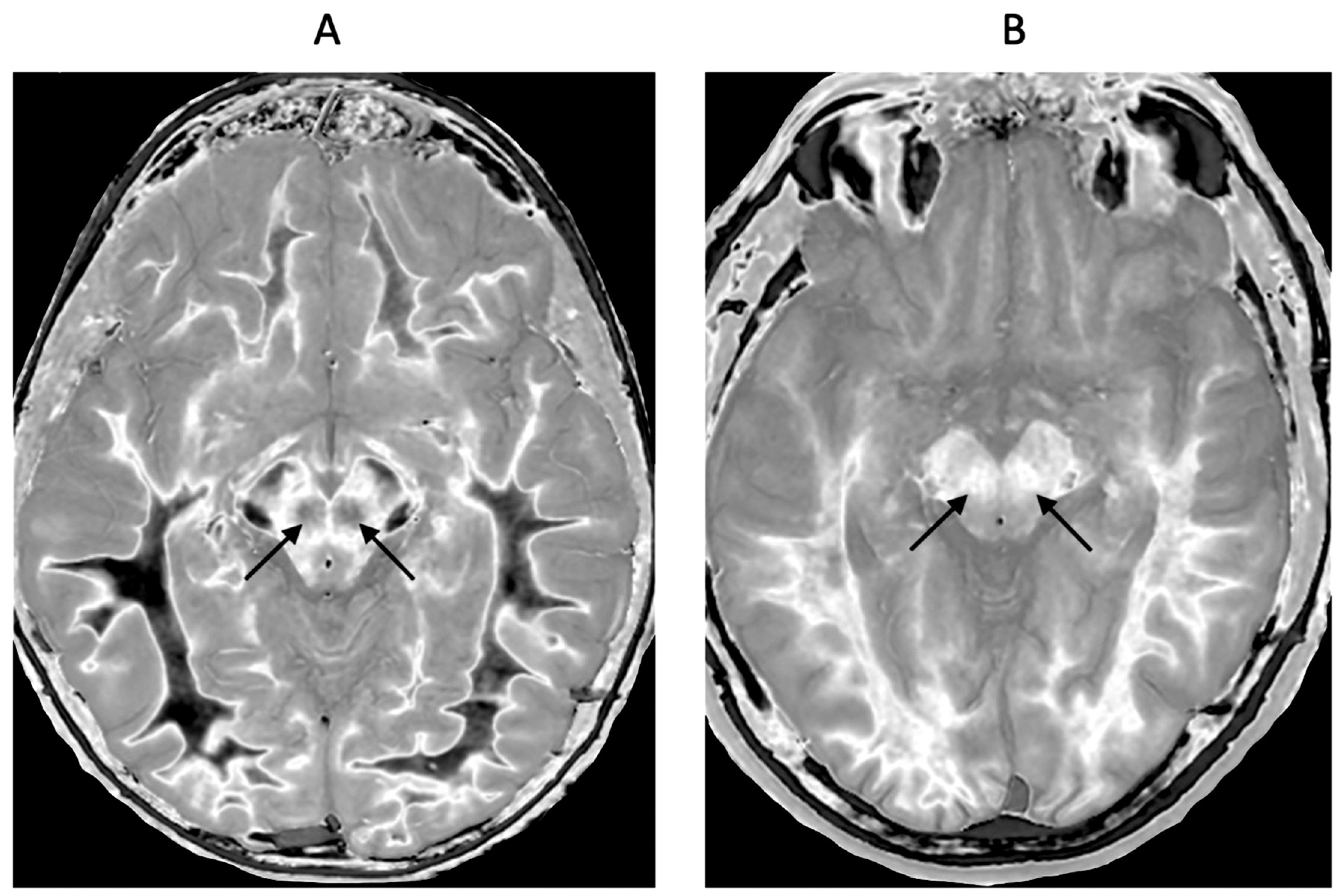
Figure 15.
41-year-old female patient with MS in remission. 2D T2-wSE (A) and narrow mD dSIR (B) images at the same level. No abnormality is seen in (A). A focal lesion is seen in (B) (long narrow white arrow) and the corticospinal tracts show a high signal (short narrow white arrows). In addition there is patchy increased signal in white matter (short thick white arrows) with only a small region showing a normal or near normal low signal appearance (long black arrow). High contrast and high spatial resolution contrast are seen at the boundaries between normal white matter and normal gray matter in (B). These features are less obvious in areas where the white matter has abnormal high signal.
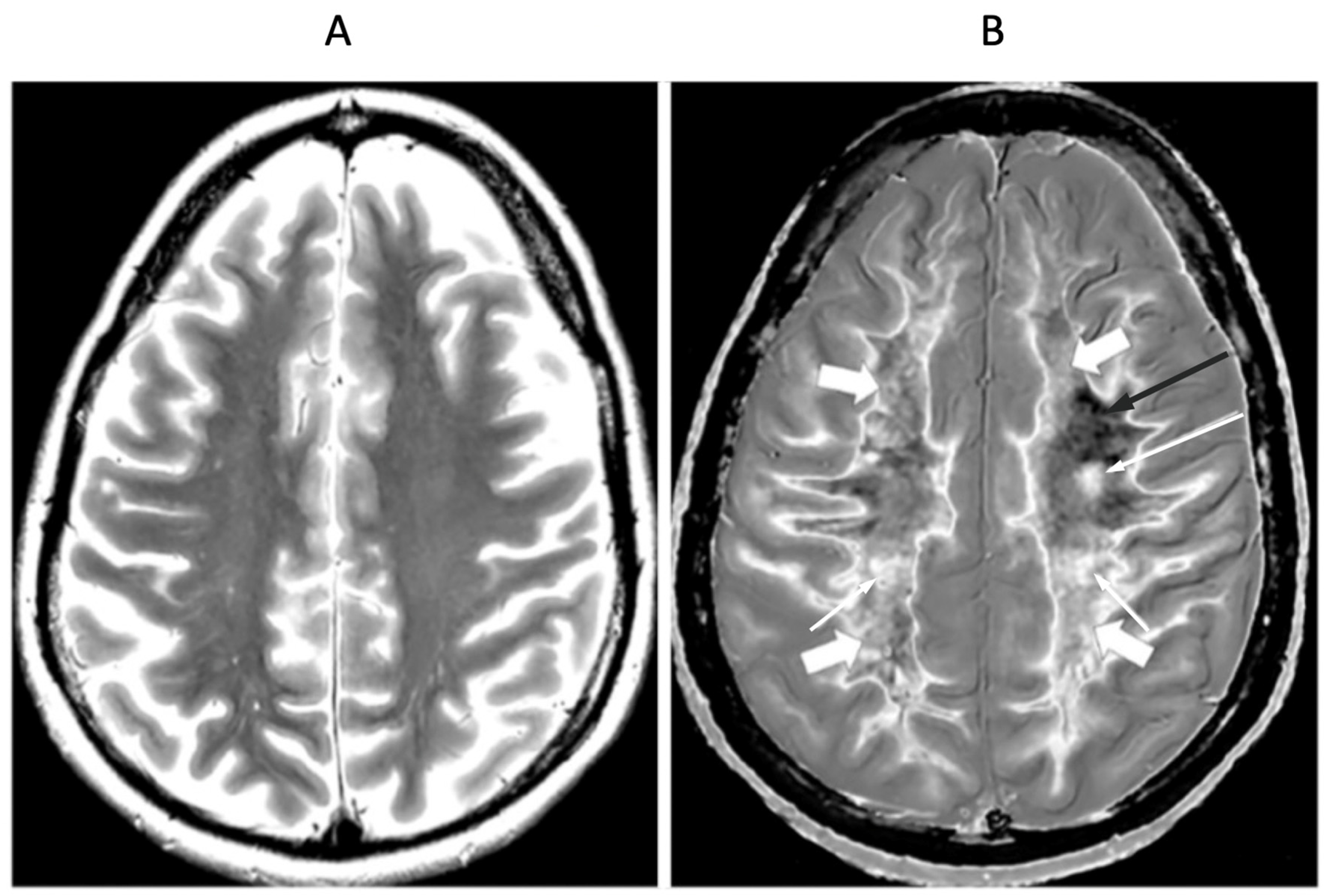
Figure 16.
32-year-old female with MS during a relapse. T2-FLAIR (A), synthetic narrow mD dSIR (B) and filtered gradient echo (C) images. On the T2-FLAIR image (A), one lesion is seen (long arrow). The surrounding white matter appears normal. On the dSIR image (B), the lesion shown on the T2-FLAIR image is seen (long arrow) as well as six other lesions (short arrows). High signal boundaries around lesions are also seen in (B). Some of these lesions show paramagnetic rims on the filtered gradient echo image (arrows) in (C). In addition, most of the white matter in (B) is high signal corresponding to a high grade 4/5 whiteout sign [1]. The whiteout sign is not seen on the T2-FLAIR image (A).
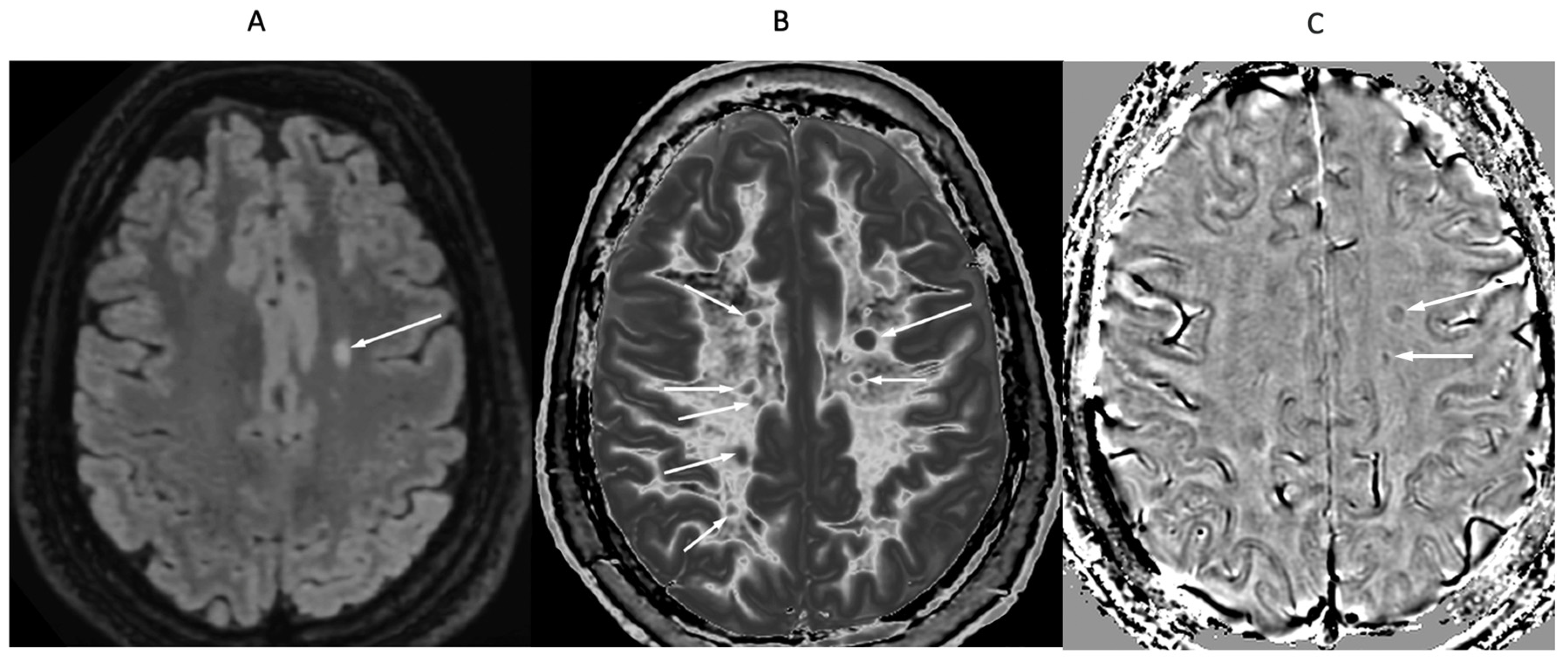
Figure 17.
24-year-old female patient with MS in remission (TIs = 350 ms, TIi = 500 ms). Narrow mD dSIR (A) and composite (T1 and T2) cdSIR (TIs/TEs = 350/7 and 80 ms; TIi/TEi = 500/7 ms) (B) images. A leukocortical lesion is seen on the dSIR image (A) and with higher contrast on the cdSIR image in (B) (arrows). White matter and gray matter boundaries are higher contrast and narrower on the composite filter cdSIR image (B). Also white matter is more uniformly low signal in (B). These features are consistent with the attenuation of the first IR TIs filter signal increasing contrast and narrowing boundaries at the positive pole and decreasing these at the negative pole as shown in Figure 10A.
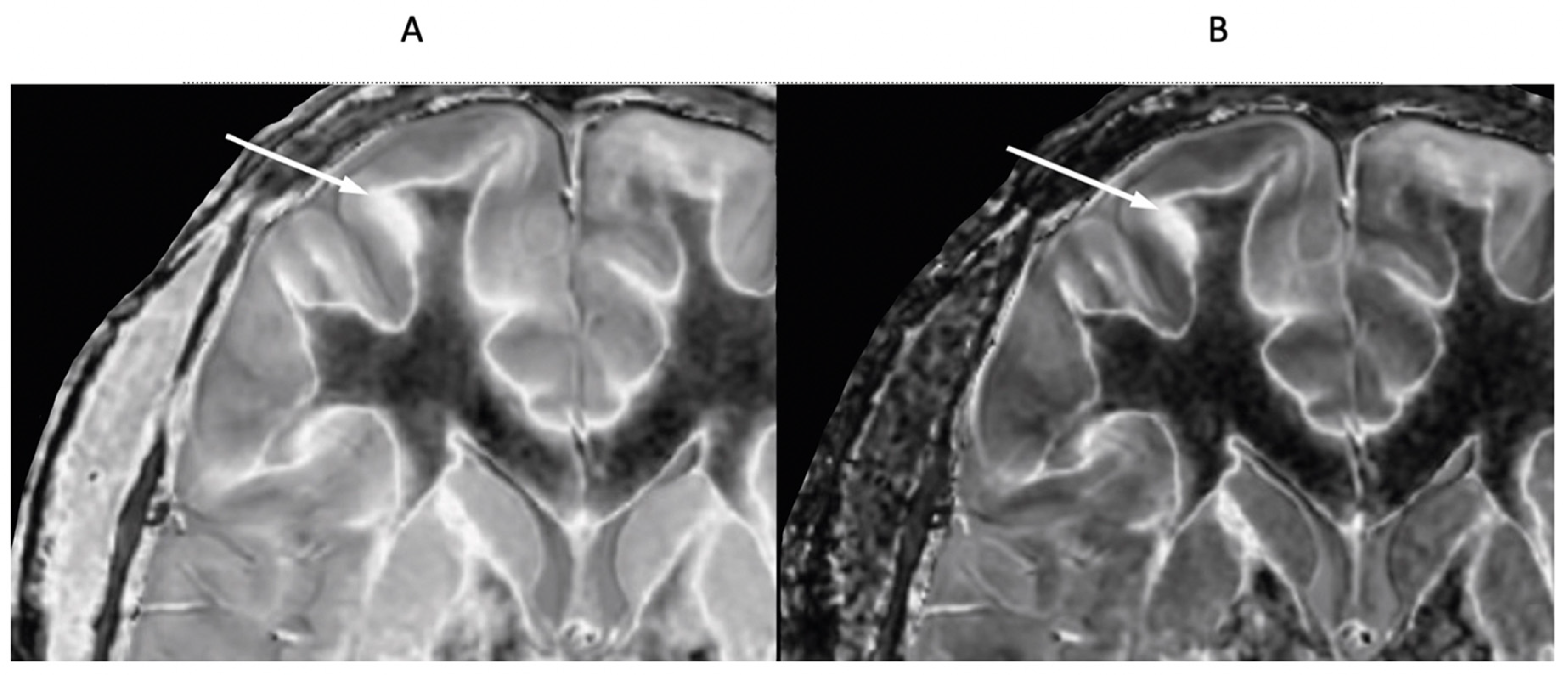
Figure 18.
76-year-old female patient in remission with a diagnosis of MS. Sagittal 3D T2-FLAIR (A) and 3D wide mD dSIR (B) images. The T2-FLAIR image shows a poorly defined area of increased signal in the cervical cord (arrow). The dSIR image shows a high contrast lesion with sharply defined ("punched out") boundaries in the cervical cord (lower three arrows). This is much more extensive than in (A). An additional lesion is seen in the medulla on the dSIR image in the region of the area postrema (highest arrow) (B) but not on the T2-FLAIR image (A). The extended lesion in the cervical cord and the lesion in the medulla raise the possibility of neuromyelitis spectrum disorder. Other conventional sequences such as MP-RAGE, T2-wSE or STIR may perform better than T2-FLAIR in the cervical cord.
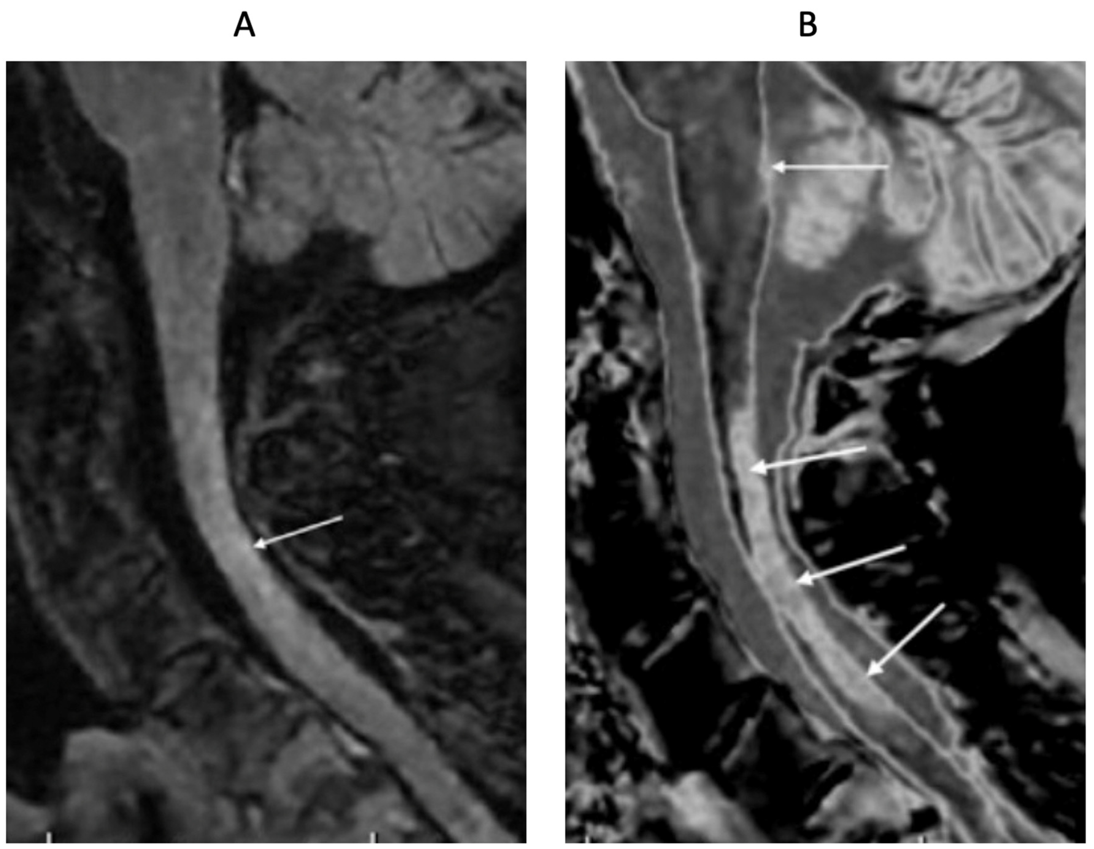
Figure 19.
51-year-old male patient with methamphetamine substance use disorder after one month's abstinence (A) and after nine months' abstinence (B). Matched narrow mD dSIR images. In (A) there is extensive high signal in the white matter of the cerebral hemispheres with only small areas of normal or near normal white matter (dark) at the periphery of the white matter (whiteout sign, grade 4 out of 5). After nine months’ abstinence (B), the high signal areas in (A) have markedly regressed. There is some intermediate signal in the more central white matter and lower signal in the peripheral white matter (whiteout sign grade 2 out of 5, where grade 1 is normal). No abnormality was seen in either examination on the corresponding T2-FLAIR images. A previous mTBI in the patient may have been a confounder.
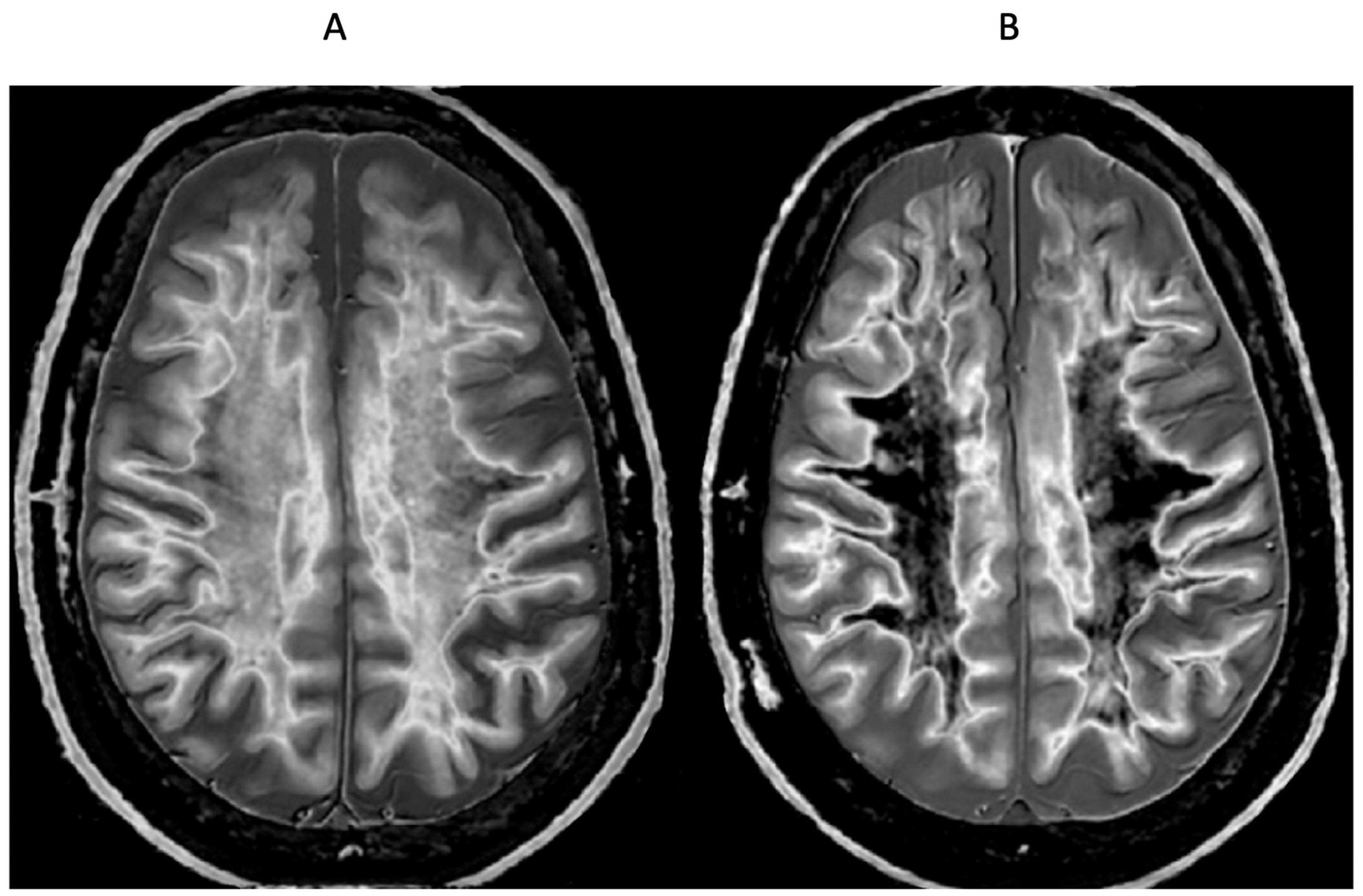
Figure 20.
72-year-old male patient with Parkinson's disease. 2D narrow mD dSIR image (A) with insets of anterior left cortex (B) and thalami (C). There is high signal in the superficial layer of the cortex at multiple sites (bilaminar cortex signs) which are more obvious on the inset (white arrows) (B). There are circular appearances in the thalami, putamen and heads of the caudate nuclei (bubble signs) which are more obvious on the inset (e.g., black arrows) (C). The bubble sign is due to focal reductions in T1 probably from the presence of free iron. The thalamic signal is slightly higher medially compared with laterally unlike the appearance of the normal thalamus in the 18-year-old patient shown in Figure 12B.
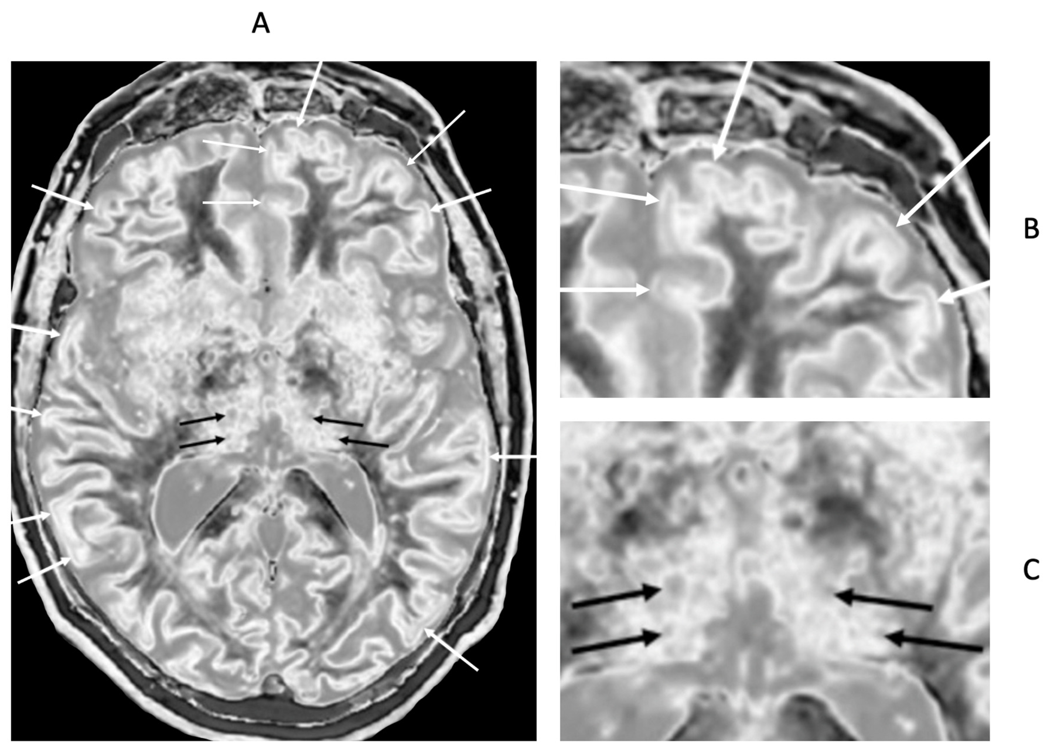
Figure 21.
65-year-old female with a glioma (not shown) post chemotherapy. Parasagittal T2-FLAIR (A) and synthetic narrow mD dSIR (B) images. On the T2-FLAIR image no abnormality is seen. On the dSIR image (B), the white matter has a high signal corresponding to a high grade whiteout sign. This includes the cerebellar white matter which is similar in intensity to the cerebral white matter. There is some sparing of the peripheral white matter in (B).
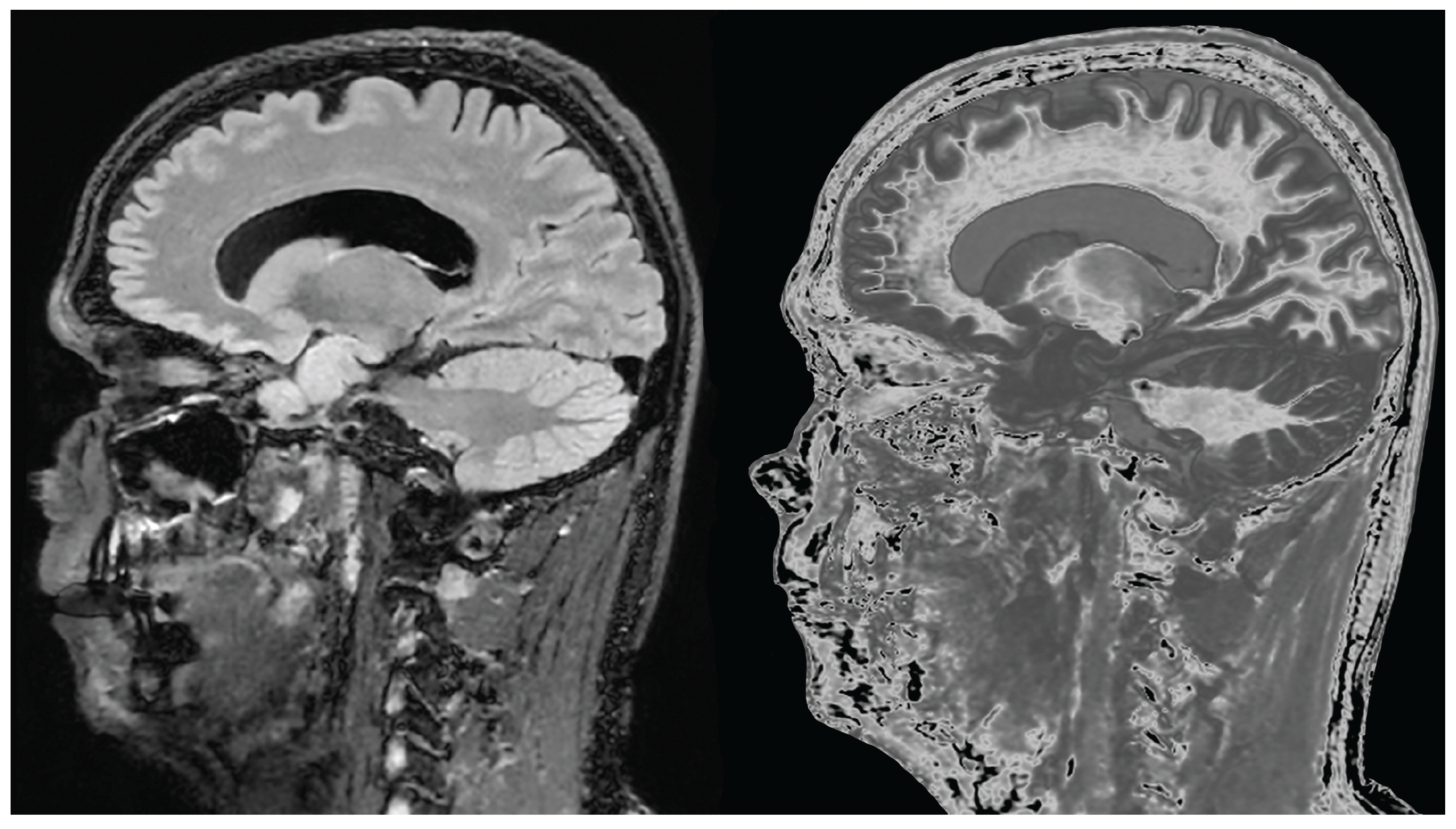
Figure 22.
46-year-old normal control. dSIR (A) and lSIR (B) images with insets of anterior left cortex dSIR in (C) and anterior left cortex lSIR in (D). The boundaries between white matter and gray matter are seen with higher contrast and the contrast is seen with higher spatial resolution in (B) and (D) compared with (A) and (C). Bilaminar cortex signs are also seen with higher contrast and spatial resolution in (B) and (D) (white arrows). There are also small bubble signs in the putamen and medial thalamus which are better seen on the lSIR image (B) compared with the dSIR image (A).
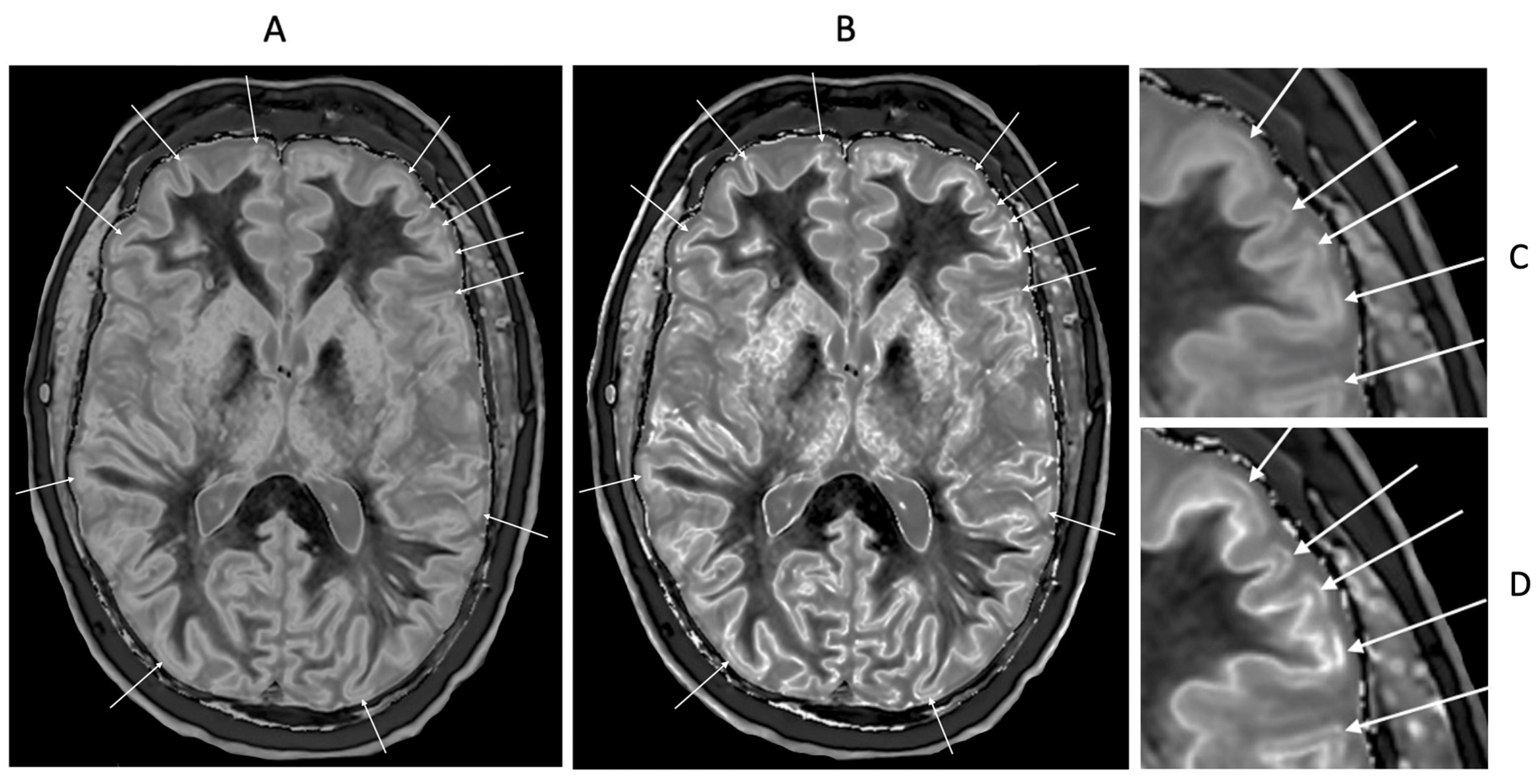
Figure 23.
41-year-old female patient with MS. A leukocortical lesion in the right medial frontal region is shown on the narrow mD dSIR image (A) and a matching lSIR image (B) (arrows). There are also left to right profiles with signal plotted against position (in mm) for the dSIR (blue) and lSIR (orange) images (C) at the level of the horizontal arrows shown in (A) and (B). No boundary between white matter and gray matter is seen within the lesion in (A). A disrupted high signal boundary between white matter and gray matter is seen in the lesion in (B). The lSIR profile (orange) has higher signal and steeper slopes than the dSIR profile (blue) in (C). The difference in signal (or contrast) achieved for the same change in position is generally greater with the lSIR filter i.e., the contrast shown on the lSIR image generally has a higher spatial resolution.
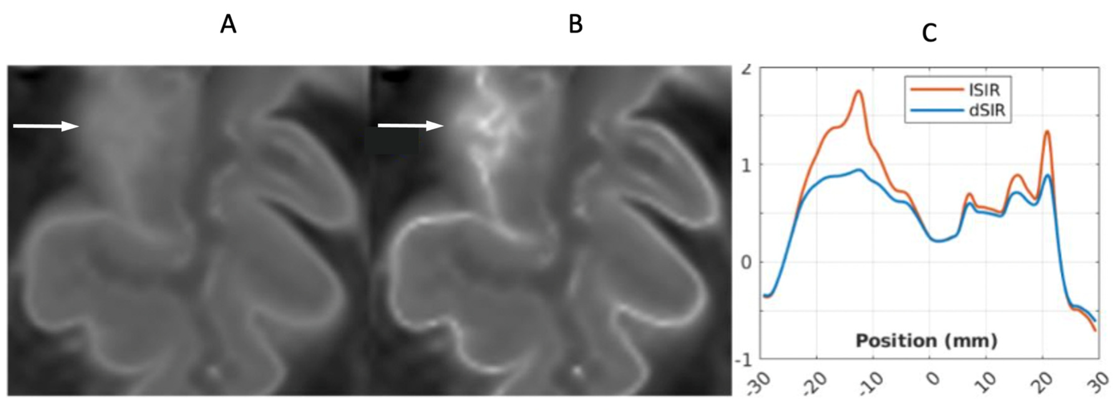
Figure 24.
Thalamus. dSIR narrow mD (TIs = 350 ms and TIi = 500 ms). T1-bipolar filter for normal appearance, abnormal increase in T1 in lateral thalamic gray matter within the hD with loss of contrast with medial thalamic gray matter (striped green arrow), and subsequent decrease in T1 to normal with restoration of contrast with medial thalamic gray matter (solid green arrow). The normal thalamus gray matter shows a decrease in T1 from medial (TGmed) to lateral (TGlat) (highest horizontal negative solid green arrow) and corresponding positive contrast (first vertical positive blue arrow). With disease there is an increase in T1 in the lateral thalamus (middle horizontal positive striped green arrow) with a loss of contrast with the medial thalamus (blue circle). With later regression of this and return of the T1 difference between the lateral and medial thalamus to normal (lowest negative solid green arrow), normal positive contrast is seen between the medial and lateral thalamus (second vertical positive blue arrow).
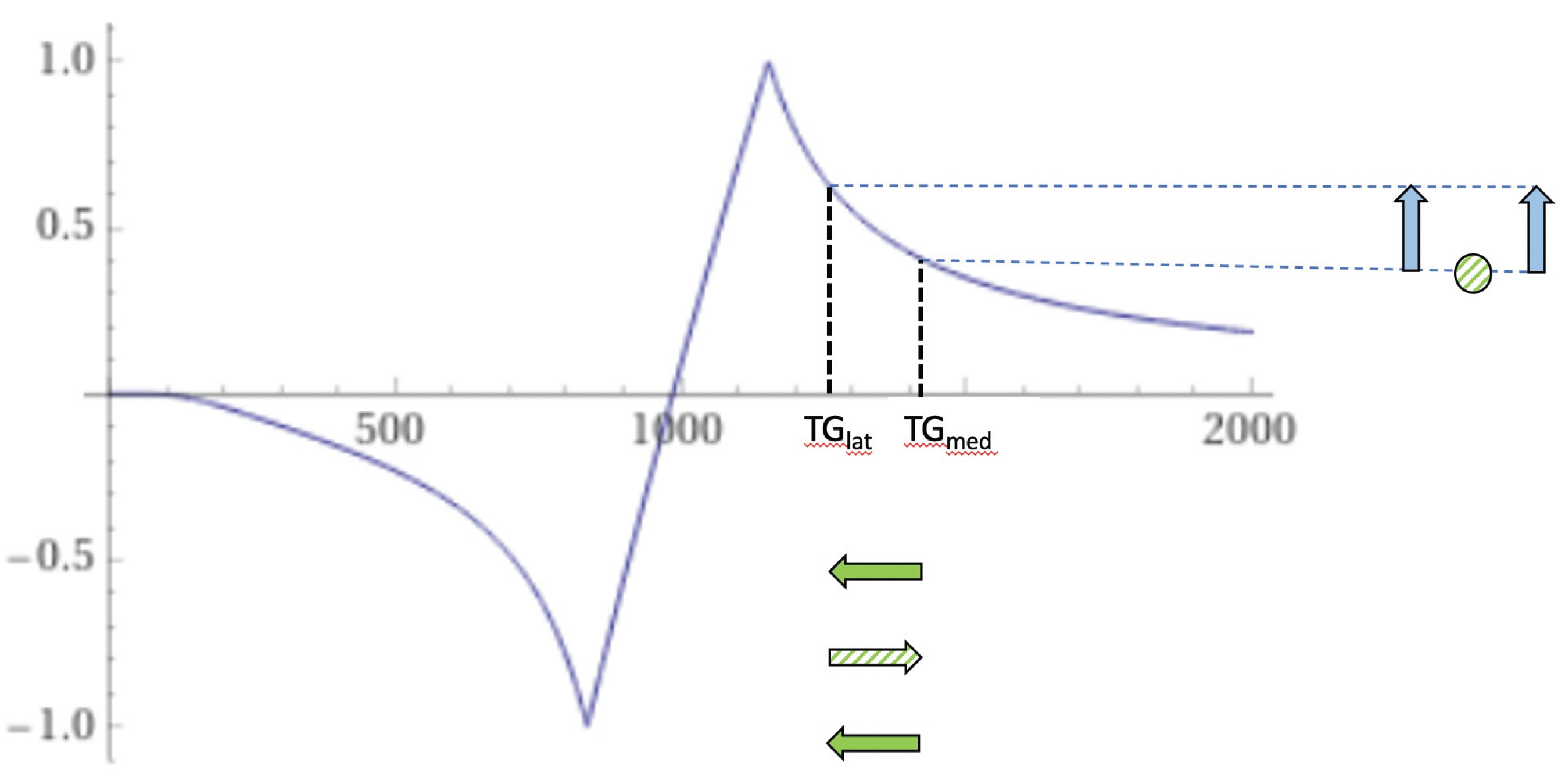
Figure 25.
Thalamus. Narrow mD (TIs = 350 ms and TIi = 500 ms). dSIR T1-bipolar filter for a larger abnormal decrease in T1 in lateral thalamic gray matter from normal (TGlatnorm) to abnormal (TGlatab) extending from the hD through the signal peak to the mD (horizontal negative green arrow). Signal in the lateral thalamus is highest where there is partial volume effect between abnormal and normal gray matter of the thalamus (TGlatab/TGlatnorm) (longer vertical blue arrow). Signal from abnormal lateral thalamus in the middle Domain (TGlatab) (shorter blue arrow) is less than the signal in the lateral thalamus at the boundary between normal and abnormal thalamus (longer blue arrow). The higher and lower signals (vertical blue arrows) result in a bubble sign with higher signal in the periphery where there are partial volume effects and lower signal centrally where there is only abnormal gray matter. The same argument applies to the medial thalamus.
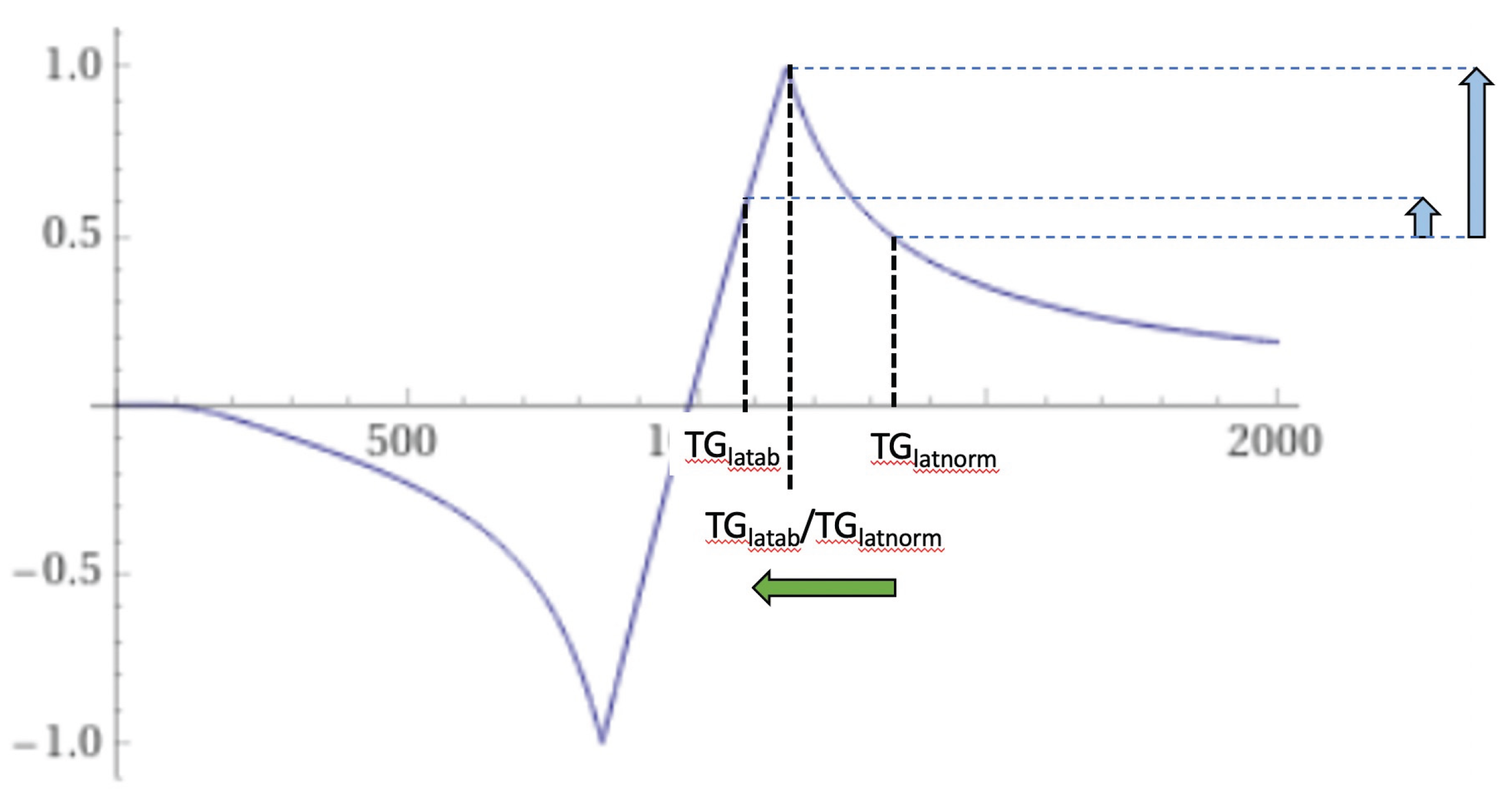

Table 1.
Pulse sequences and pulse sequence parameters used at 3T. Only 2D scans were performed on the Siemens Healthineers Skyra system.
Table 1.
Pulse sequences and pulse sequence parameters used at 3T. Only 2D scans were performed on the Siemens Healthineers Skyra system.
| # | Sequence | TR (ms) | TI (ms) | TE (ms) | Matrix size Voxel size (mm) |
Number of slices | Slice thickness (mm) |
| 1* | 2D FSE IR (for white nulling matter) | 9,192 | 350 | 7, 80 | 256 x 224 0.9 x 0.1 Z512 0.4 x 0.4 |
26 | 4 |
| 2* | 2D FSE IR (used with #1 for narrow mD dSIR) | 5,796 | 500 | 7, 80 | 256 x 224 0.9 x 0.1 Z512 0.4 x 0.4 |
26 | 4 |
| 3* | 2D FSE IR (for longer T1 nulling) | 5,796 | 600 | 7 | 256 x 224 0.9 x 0.1 Z512 0.4 x 0.4 |
26 | 4 |
| 4* | 2D FSE IR (used with #1 for wide mD dSIR) | 5,796 | 800 | 7 | 256 x 224 0.9 x 0.1 Z512 0.4 x 0.4 |
26 | 4 |
| 5 | 3D BRAVO (for white matter nulling) | 2,000 | 400 | 6 | 256 x 256 0.8 x 0.8 Z512 |
220 | 0.8 |
| 6 | 3D BRA VO (used with #5 for wide mD dSIR) |
2,000 | 800 | 6 | 256 x 256 0.8 x 0.8 Z512 |
220 | 0.8 |
| 7* | 2D T2-FLAIR | 6,300 | 1,851 | 102 | 320 x 240 0.7 x 0.7 Z512 0.4 x 0.4 |
26 | 4 |
| 8 | 3D T2-FLAIR | 6,300 | 1,850 | 102 | 256 x 256 0.8 x 0.8 Z512 0.6 x 0.6 |
252 | 0.8 |
| 9 | 3D susceptibility weighted | 40 |
- | 32 | 300 x 300 0.8 x 0.8 Z512 |
110 | 2 |
Z = zipped. * = positionally matched for slice position, slice thickness, slice number, field of view and interpolated matrix size.
Table 2.
Directly acquired tissue property bipolar filters.
| Bipolar filter | Reverse bipolar filter | Tissue properties single (upper) composite (lower) |
|---|---|---|
| SIR | rSIR | T1 |
| dSIR cdSIR |
drSIR cdrSIR |
T1 T1; T2, T2, D*, c and/or MT |
| lSIR clSIR |
lrSIR clrSIR |
T1 T1; T2, T2*, D*, c and/or MT |
Table 3.
Signal equations for bipolar filters and other functions.
| # | Filter, other functions | Signal Equation | Figure # |
|---|---|---|---|
| 1 | IR, TIs | STIs = 1-2e-TIs/T1 | 3,4,5 |
| 2 | IR, TIi | STIi = 1-2e-TIi/T1 | 3,4,5 |
| 3 | SIR | SSIR = STIs - STIi | 5 |
| 4 | dSIR |
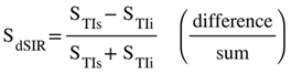 |
6,9 |
| 5 | dSIR |
 (in lD and hD) (in lD and hD)ΔTI = TIi – TIs 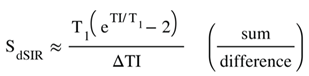 (in mD) (in mD) |
6,9 |
| 6 | cdSIR |
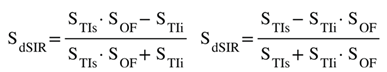
|
10 |
| 7 | cdSIR, SOF | SOF = ±e-DTE/T2, ± e-DTE/T2*, ±e-DbD*, etc | 10 |
| 8 | dSIR, SdSIR | (in mD) | 6 |
| 9 | dSIR, T1 | (in mD) | 6 |
| 10 | lSIR | SlSIR = ½(ln STIs - ln STIi) | 8,9 |
| 11 | clSIR | 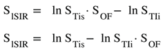 |
|
| 12 | clSIR, lSIR |
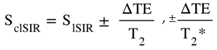 , ±DbD*, etc , ±DbD*, etc |
|
| 13 | lSIR, dSIR† | SlSIR = atanh SdSIR (in mD) | 9 |
| 14 | dSIR, T1D†† |
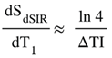 (in mD) (in mD) |
6,9 |
| 15 | lSIR, T1D ††† |
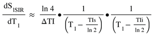 (in mD) (in mD) |
9 |
† SlSIR is the inverse hyperbolic tangent of SdSIR in the mD. ††  is the T1 derivative (T1D) of SdSIR and gives the slope of dSIR filter in the mD which is essentially constant and equal to
  (Figure 9). †††
  is the T1 derivative (T1D) of the SlSIR filter in the mD which varies. It has values of minus or plus infinity when
  and
and  respectively (Figure 9).
is the T1 derivative (T1D) of SdSIR and gives the slope of dSIR filter in the mD which is essentially constant and equal to (Figure 9). ††† is the T1 derivative (T1D) of the SlSIR filter in the mD which varies. It has values of minus or plus infinity when and respectively (Figure 9).
Disclaimer/Publisher’s Note: The statements, opinions and data contained in all publications are solely those of the individual author(s) and contributor(s) and not of MDPI and/or the editor(s). MDPI and/or the editor(s) disclaim responsibility for any injury to people or property resulting from any ideas, methods, instructions or products referred to in the content. |
© 2025 by the authors. Licensee MDPI, Basel, Switzerland. This article is an open access article distributed under the terms and conditions of the Creative Commons Attribution (CC BY) license (http://creativecommons.org/licenses/by/4.0/).
Copyright: This open access article is published under a Creative Commons CC BY 4.0 license, which permit the free download, distribution, and reuse, provided that the author and preprint are cited in any reuse.


