Submitted:
28 May 2025
Posted:
28 May 2025
Read the latest preprint version here
Abstract
Complex networks model the structure and function of critical technological, biological, and communication systems. Network dismantling---the targeted removal of nodes to fragment a network---is essential for analyzing and improving system robustness. Existing dismantling methods suffer from key limitations: they depend on global structural knowledge, exhibit slow running times on large networks, and overlook the network’s latent geometry. However, it has been shown that complex systems run their dynamics on a manifold in a latent geometric space. Motivated by these findings, we introduce Latent Geometry-Driven Network Automata (LGD-NA), a novel framework that leverages local network automata rules to approximate effective link distances between interacting nodes. LGD-NA is able to identify critical nodes and capture latent manifold information of a network for effective and efficient dismantling. We show that this latent geometry-driven approach outperforms all existing dismantling algorithms, including machine learning methods such as graph neural networks. We also find that a simple common-neighbor-based network automata rule achieves near state-of-the-art performance, highlighting the effectiveness of minimal local information for dismantling. LGD-NA is extensively validated on the largest and most diverse collection of real-world networks to date (1,475 real-world networks across 32 complex systems domains) and scales efficiently to large networks via GPU acceleration. Our results confirm latent geometry as a fundamental principle for understanding the robustness of real-world systems, adding dismantling to the growing set of processes that network geometry can explain.
Keywords:
network robustness
; network dismantling
; network geometry
; network science
; complex systems
; network automata
; graphs
; network topology
1. Introduction
Complex networks shape every aspect of human life, driving critical systems such as technological infrastructures, information systems, and biological processes [5]. Their fundamental role makes it crucial to understand their vulnerability to targeted attacks. Disrupting these networks can have far-reaching effects, triggering phenomena such as epidemic outbreaks, infrastructure failures, financial crises, and misinformation propagation [6,7].
A targeted attack on a network—known as network dismantling—aims to disrupt its structural integrity and functional capacity by identifying and removing a minimal set of critical nodes that fragment it into isolated sub-components [6]. Designing effective dismantling strategies is essential, as they provide insights for improving the robustness of these critical networks.
Efficient network dismantling is challenging because identifying the minimal set of nodes for optimal disruption is an NP-hard problem—no known algorithm can solve it efficiently for large networks [6]. This difficulty arises not only from the prohibitively large solution space but also from the structural complexity of real-world networks, which exhibit heterogeneous, fat-tailed connectivity [8,9,10,11] and intricate organizations such as modular and community structures [12,13], hierarchies [14,15], higher-order structures [16,17], and a latent geometry [1,18,19,20,21,22,23].
Node Betweenness Centrality (NBC) is a network centrality measure [24] that quantifies the importance of a node in terms of the fraction of the shortest paths that pass through it. NBC-based attack, where nodes are removed in order of their betweenness centrality, is considered one of, if not the best, method for network dismantling [25,26,27,28]. However, like many other dismantling techniques, it requires global knowledge of the entire network topology, and its high computational cost limits its scalability to large networks. These limitations are shared by many other state-of-the-art dismantling methods, which additionally rely on black-box machine learning models, and are rarely validated across large, diverse sets of real-world networks (see Table 1, Table A3, and Table A2).
Latent geometry has been recognized as a key principle for understanding the structure and complexity of real-world networks [18,19,20,21,23,29,30]. It explains essential features such as small-worldness, degree heterogeneity, clustering, and navigability [18,19,21], and drives critical processes like efficient information flow [20,29,30,31].
Recent work by Muscoloni et al. (2017) [1] revealed that betweenness centrality is a global latent geometry estimator: it approximates node distances in an underlying geometric space. They also introduced Repulsion-Attraction network automata rule 2 (RA2), a local latent geometry estimator that uses only first-neighbor connectivity. RA2 performed comparably to NBC in tasks such as network embedding and community detection, despite relying solely on local information.
This raises the first question: can latent geometry—whether estimated globally or locally—guide effective network dismantling? If complex systems run on a latent manifold, estimating it may offer a more efficient way to disrupt connectivity.
The second question concerns efficiency: both NBC and RA2 have complexity, where N is the number of nodes and m the number of links in a network. However, RA2 is significantly faster in practice due to its use of local information and avoidance of the large running time associated with NBC’s computational overhead. This motivates exploring whether local latent geometry estimators can match the dismantling performance of global methods like NBC while offering a greater advantage in practical running time execution.
Motivated by these questions, we introduce the Latent Geometry-Driven Network Automata (LGD-NA) framework, which uses local topology estimators of latent geometry to drive the dismantling process. It achieves state-of-the-art dismantling performance on 1,475 real-world networks across 32 complex systems domains and its GPU implementation enables dismantling at large scales. Our contributions are as follows:
1. Latent Geometry-Driven (LGD) dismantling. Global LGD dismantling, such as NBC and local ones, such as RA2-based methods, estimate effective node distances on the manifold associated with the network in the latent space, capturing its geometry and exposing structural information critical for dismantling.
2. LGD Network Automata (LGD-NA). Network automata rules adopt local topology information to approximate the latent geometry distances of pairs of linked nodes in the network. The sum of the distances that a node has from its linked neighbors represents an estimation of how central a node is in the network topology. The higher this sum, the more a node dominates numerous and far-apart regions of the network, being a critical candidate for network dismantling. We show that LGD-NA consistently outperforms all other existing dismantling algorithms, including machine learning methods such as graph neural networks.
3. A simple common neighbors-based network automaton rule is highly effective. We discover that a variant of RA2, based solely on common neighbors, outperforms all other dismantling algorithms and achieves performance close to the state-of-the-art method, NBC. We refer to this variant as the common neighbor dissimilarity (CND): a minimalistic network automaton rule that acts as a local latent geometry estimator.
4. Comprehensive experimental validation. We build an ATLAS of 1,475 real-world networks across 32 complex systems domains, which is the largest and most diverse collection of real-world networks to date. We evaluate LGD-NA on this ATLAS, comparing with state-of-the-art methods, proving the effectiveness of LGD-NA in a wide variety of real-world settings
5. GPU-acceleration. We implement GPU acceleration for LGD-NA, enabling remarkable running time advantages in dismantling on networks significantly larger than those manageable by the state-of-the-art method, NBC.
2. Related Work
2.1. Latent Geometry of Complex Networks.
Many real-world networks are shaped by latent geometric manifolds of the complex systems that govern their topology and dynamics. These hidden geometries explain essential structural features such as small-worldness, degree heterogeneity, clustering, and community structure [1,18,19,21,23,38,39]. The underlying metric space is not only descriptive but functional: it facilitates efficient routing and navigation with limited global knowledge [20,29,30,31]. Such properties emerge consistently across diverse systems, including biological, social, technological, and socio-ecological networks [18,19]. Latent geometries also enable predictive modeling of dynamical processes such as network growth [23,39,40], and epidemic spreading [22].
2.2. Latent Geometry Estimators
Latent geometry estimators assign edge weights to approximate linked nodes’ pairwise distances in the hidden geometric manifold. Among them, network automata rules based on the Repulsion-Attraction (RA) criterion use only local topological information to infer proximity in the latent space [1]. RA is grounded in the theory of network navigability [29], which posits that nodes with many non-overlapping neighbors tend to occupy distant regions in the latent space. Edges between such nodes receive higher dissimilarity scores due to strong repulsion, while those with many common neighbors are scored lower due to attraction.
RA1 and RA2 are network automata rules for approximating linked nodes’ pairwise distances on the latent manifold of a complex network. These rules are categorized as network automata because they adopt only local information to infer the score of a link in the network without the need for pre-training of the rule. Note that RA1 and RA2 are predictive network automata that differ from generative network automata, which are rules created to generate artificial networks [8,39,40].
They were introduced to serve as pre-weighting strategies for approximating angular distances associated with node similarities in hyperbolic network embeddings [1]. RA2 performed slighter better than RA1, so for this reason we will only consider RA2 in this study. RA2 defines dissimilarity between nodes i and j as:
where is the number of common neighbors of nodes i and j, and and are the external degrees of i and j, representing the count of neighbors of i and j which are not involved in the common neighbors interactions.
In the same work, Muscoloni et al. also showed that betweenness centrality is a global latent geometry estimator. By comparing it with RA2, they demonstrated that both global (betweenness centrality) and local (RA) estimators can effectively capture latent geometry, achieving strong results in network embedding and community detection. See Table A1 for a comparison of estimators and Figure A1 for illustrative examples.
2.3. Topological centrality measures
Degree, betweenness centrality, and their variants have all been used in the majority of dismantling studies [6], with betweenness centrality [25,26,27,28] having been found to be the most effective strategy when applying dynamic dismantling, meaning the scores are recomputed after every step. Degree centrality ranks nodes by their number of neighbors, and betweenness centrality [24] counts how frequently a node lies on shortest paths. Other centrality variants include eigenvector centrality [41], which gives higher scores to nodes connected to other influential nodes. PageRank [42], based on a random walk model and originally developed for ranking web pages, favors nodes that receive many and high-quality links. Beyond these classical measures, several centrality indices have been specifically developed to capture aspects of network resilience. Fitness centrality [26], adapted from economic complexity theory, evaluates node importance through the capabilities of neighbors while penalizing connections to weak nodes. DomiRank [25] centrality models a competitive dynamic in which nodes gain or lose dominance, or importance, based on the relative strength of their neighbors. Resilience centrality [35], derived from a dynamical systems reduction, quantifies how a node’s removal alters the system’s resilience, incorporating both degree and weighted nearest-neighbor degree. See Table A2 for a full comparison of topological centrality measures.
2.4. Statistical and Machine Learning Network Dismantling
We focus on network dismantling for targeted attacks, where the goal is to fragment a network as efficiently as possible by removing selected nodes. Message passing-based methods such as Belief Propagation-guided Decimation (BPD) [4] and Min-Sum (MS) [2] use message-passing algorithms to decycle the network and then fragment the resulting forest with a tree-breaker algorithm, while CoreHD [32] achieves decycling by iteratively removing the highest-degree nodes from the 2-core of the network and also includes a tree-breaker algorithm. Decycling and dismantling are, in fact, closely related tasks, as a tree (or a forest) can be dismantled almost optimally [2]. Generalized Network Dismantling (GND) [34] targets nodes that maximize an approximated spectral partitioning. Collective Influence (CI) [3] targets nodes with maximal influence on their neighborhoods, and Explosive Immunization (EI) [33], uses explosive percolation dynamics. Machine learning-based methods include Graph Dismantling with Machine Learning (GDM) [36], which trains graph neural networks to predict optimal attack strategies in a supervised manner. FINDER [43] uses reinforcement learning instead to autonomously learn dismantling strategies without needing labeled data. CoreGDM [37] combines ideas from CoreHD and GDM as it attacks the 2-core of the network but uses machine learning models trained on optimal dismantling solutions to guide node removal. See Table A3 for a full comparison of dismantling methods.
3. Latent Geometry-Driven Network Automata
We introduce the Latent Geometry-Driven Network Automata (LGD-NA) framework. LGD-NA adopts a network automaton rule, such as RA2, to estimate latent geometric linked node pairwise distances and to assign edge weights based on these geometric distances. Then, it computes for each node its network centrality as a sum of the weights of adjacent edges. The higher this sum, the more a node dominates numerous and far-apart regions of the network, becoming a prioritized candidate for a targeted attack in the network dismantling process. This prioritized node is then removed from the network, and the procedure is iteratively repeated until the network is dismantled. The reinsertion phase can optionally be applied after dismantling to improve performance by reinserting nodes that were not relevant to the dismantling process. See Figure 1 for a full breakdown of the LGD-NA framework.
3.1. Latent Geometry-Driven dismantling
Our first contribution is Latent Geometry-Driven (LGD) dismantling, where any function can be used to estimate edge weights that represent effective distances between nodes, capturing the network’s underlying latent geometry. These inferred weights are used to construct a dissimilarity-weighted network, encoding a hidden geometric structure beneath the observable topology and allowing the dismantling process to prioritize the more important nodes according to their geometric centrality in the latent manifold.
Latent geometric structures have been shown not only to explain key properties of complex networks [19], but also to support the understanding of dynamical processes such as navigation, routing [20,29,30,31], and epidemic spreading [22]. They have also been successfully applied to network embedding and community detection [1]. Building on the idea that network geometry captures essential structural and dynamical properties of complex systems, LGD dismantling is guided by a geometric intuition about how nodes connect distant regions in the latent space. If two nodes are connected to many different nodes but have little overlap in their neighborhoods, they are likely to be far apart in the network’s latent space. An edge between them therefore, connects distant regions of the network. A node that has many such edges plays a central role in holding the network together, as it links otherwise separate areas. We propose that removing those geometrically central nodes is an effective way to fragment the network.
Muscoloni et al. (2017) [1] also offered evidence that betweenness centrality can be used as a latent geometry estimator, hence, NBC is a global topology centrality measure which can be used for latent geometry-driven dismantling.
3.2. LGD Network Automata
Our second contribution is the introduction of a network automaton framework for LGD dismantling. In this framework, node importance is estimated by aggregating edge geometric weights into node strengths, and the network is dismantled iteratively by removing the nodes with the highest strength and all their edges. The underlying intuition is that nodes that connect to many external, non-overlapping regions are geometrically central and thus more structurally important, leading to higher strength values.
Formally, we begin with an undirected, unweighted network without isolated components. A network automaton rule, such as RA2, that is able to adopt local topology to estimate latent geometry, is applied to assign a weight to the edge between node i and node j, representing the estimated geometric distance between the two nodes. We get a dissimilarity-weighted network from these edge weights. The strength of node i is then calculated by summing the geometric weights of all its edges, that is, the weights to all its neighbors in the set :
In this paper, we adopt three types of LGD network automata rules. The first rule is RA2, which was proposed by Muscoloni et al. (2017) [1] for hyperbolic network embedding purposes. The second rule is proposed in this study as an ablation test of the RA2 rule. It is the denominator of the RA2, and we call it common neighbors dissimilarity (CND), and is defined as:
where is the number of common neighbors between nodes i and j. Here, the lower the number of common neighbors two interacting nodes have, the more geometrically distant they are, and thus a higher edge weight is assigned between these two nodes.
The rationale for proposing a network automaton rule based only on the common neighbors denominator term of RA2 is to account for the mere attraction between a node and its neighbors. Neglecting the repulsion part associated with the external links (the numerator of RA2) makes sense in a dismantling task because any time we compute the common neighbors of a seed node with one of its neighbors, we indirectly account for the exclusion of nodes that are not in the topological neighborhood of the seed node. For completeness, we also investigate a third rule as an ablation test of RA2 in which we consider only the external links term in the RA2 numerator, expecting that the mere RA2 numerator should also work, but not as well as the common neighbor-based denominator. Indeed, a previous study offers evidence that common neighbors are among the topological features most associated with community organization and mesoscale network geometry [44].
4. Experiments
4.1. Evaluation Procedure
We evaluate all dismantling methods using a widely accepted procedure in the field of network dismantling [6]. For each method, nodes are removed sequentially according to the order it defines. After each removal, we track the normalized size of the Largest Connected Component (LCC), defined as the ratio , where is the total number of nodes in the original network and is the number of nodes in the largest component after x removals. This process continues until the LCC falls below a predefined threshold. A commonly accepted threshold in dismantling studies is 10% of the original network size [6]. To quantify dismantling effectiveness, we compute the Area Under the Curve (AUC) of the LCC trajectory throughout the removal process, which records the normalized LCC size at each step. A lower AUC indicates a more efficient dismantling, as it reflects an earlier and sharper disruption of network connectivity. The AUC is computed using Simpson’s rule. See Figure A2, Figure A4, Figure A7, and Figure A8 for visual illustrations of the LCC curve.
4.2. Optional Reinsertion Step
After reaching the dismantling threshold, we optionally perform a reinsertion step to lower the dismantling cost by reintroducing nodes removed but were ultimately unnecessary. We test three reinsertion techniques introduced by previous dismantling studies: Braunstein et al. (2016) [2] chooses the node ending up in the smallest component; Morone et al. (2016) [3] selects the node connecting the fewest components; Mugisha and Zhou (2016) [4] prioritizes nodes causing the smallest LCC increase. Reinsertion can significantly improve dismantling performance; recent work shows that simple heuristics with reinsertion can match or outperform complex algorithms that include reinsertion by default [45]. As a result, we enforce two constraints to ensure the reinsertion step does not override the original dismantling method: (1) reinsertion cannot reinsert all nodes to recompute a new dismantling order, and (2) reinsertion must use the reverse dismantling order as a tiebreak. If a method includes reinsertion by default, we also evaluate its performance without reinsertion for a fair comparison. See Table A4 for a full comparison of reinsertion methods.
4.3. ATLAS Dataset
Our fourth contribution is the breadth and diversity of real-world networks tested in our experiments, demonstrating the generality and robustness of LGD-NA across domains and scales.
We build an ATLAS of 1,475 real-world networks across 32 complex systems domains, which is the largest and most diverse collection of real-world networks to date used for testing in network dismantling studies. We first test all methods across networks of up to 5,000 nodes and 205,000 edges without reinsertion (), and 38,000 edges with reinsertion (). To assess the practical running time of the best performing methods, we evaluate NBC and RA2 on even larger networks of up to 23,000 nodes and 507,000 edges ().
Current state-of-the-art dismantling algorithms have been evaluated on no more than 57 real-world networks (see Table 1), with most algorithms tested on fewer than a dozen. Our experiments cover 1,475 networks, representing a substantial expansion.
A key aspect of our ATLAS dataset is the diversity of network types (see Table 2). We test across 32 different complex systems domains, ranging from protein-protein interaction (PPI) to power grids, international trade, terrorist activity, ecological food webs, internet systems, brain connectomes, and road maps. Since fields vary in both the number of networks and their characteristics, we evaluate dismantling methods using a mean field approach, ensuring that fields with more networks do not dominate the overall evaluation. Also, because dismantling performance varies in scale across fields, we compute a mean field ranking to make results comparable across domains. Specifically, we rank all methods within each field based on their average AUC, then compute the mean of these rankings across all fields.
4.4. LGD-NA Performance and Comparison to Other Methods
We compare our Latent Geometry-Driven Network Automata (LGD-NA) framework against the best-performing dismantling algorithms in the literature. Main results are shown in Figure 2.
First, we find that all latent geometry network automata—NBC, RA2, and its variants—achieve top dismantling performance, both with and without reinsertion. These findings show that estimating the latent geometry of a network effectively reveals critical nodes for dismantling, confirming our first contribution.
For each method, we evaluate three reinsertion strategies and report the best result. We show in Figure A3 that using different reinsertion methods does not change the mean field ranking of the dismantling methods, and in Figure A5 that the improvement in performance varies across fields and reinsertion methods (see Figure A4 for an illustrative example). We also adopt a dynamic dismantling process for the network automata rules and all centrality measures, where we recompute the scores after each dismantling step, as it consistently outperforms the static variant (see Figure A6 for an example of the improvements for CND and Figure A7 for an illustrative example).
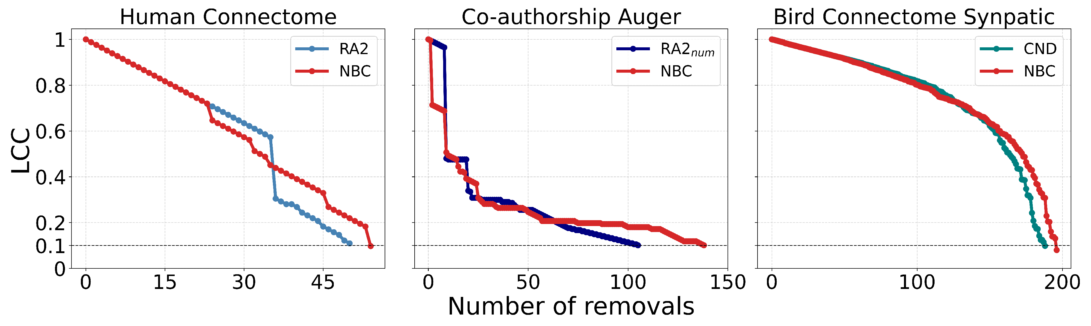
Second, we find that local network automata rules RA2, CND, and —which adopt only the local network topology around a node—are highly effective. In particular, RA2 and its variants consistently outperform all other non-latent geometry-driven dismantling algorithms, including those relying on global topological measures or machine learning. This confirms our second contribution. See Figure A2 for illustrative examples where the local network automata rules outperform NBC.
Third, we find that the simplest RA2 variant—based solely on inverse common neighbors, which we refer to as common neighbor dissimilarity (CND)—achieves the best performance among all local network automata rules. This is our third contribution and demonstrates that even minimal local topology-based information can effectively approximate latent geometry useful for effective dismantling.
LGD-NA outperforms all other methods, is robust to the inclusion or omission of reinsertion, and is validated across a large and diverse set of networks. These results strongly demonstrate the practical reliability of our latent geometry-driven dismantling framework, LGD-NA.
4.5. GPU Acceleration of LGD-NA for Large-Scale Dismantling
We implement GPU acceleration for all three LGD-NA variants by reformulating the required computations as matrix operations. On large networks, this enables a significant speedup in running time. Since the difference in running time between the three LGD-NA methods is not relevant, neither for CPU nor GPU, we report only the running time of RA2 in Figure 3. For NBC, we report only CPU running time, as its GPU implementation did not yield any speedup. On the largest network, GPU-accelerated RA2 is 130 times faster than its CPU counterpart, highlighting the inefficiency of matrix multiplication on CPU. It is also over 63 times faster than NBC running on CPU, thanks to our GPU-optimized implementation. However, as noted earlier, NBC on CPU remains faster than RA2 on CPU, again due to the limitations of CPU-based matrix operations.
Overall, while NBC achieves better dismantling performance, its high computational cost makes it impractical for large-scale use. In contrast, thanks to our GPU-optimised implementation, our local latent geometry estimators based on network automata rules are the only viable option for efficient dismantling at scale.
Here, we look at the details of our matrix operations for the LGD-NA measures. First, the common neighbors matrix is computed as
where is the adjacency matrix and ∘ denotes element-wise multiplication. Here, counts the number of paths of length two—i.e., common neighbors—between all node pairs. The Hadamard product with ensures that values are only retained for existing edges.
Next, we compute the number of external links a node has relative to each of its neighbors. Given the degree matrix , the external degree matrix is:
Each entry of represents the external degree of node i with respect to node j: the number of neighbors of i that are neither connected to j nor directly connected to j itself. Non-edges are zeroed out.
These matrices allow efficient construction of RA2 and its variants using only matrix operations:
The time complexity is , with the common neighbor matrix being the dominant operation, for dense graphs, and for sparse graphs, N being the number of nodes and m the number of links. On CPU, matrix multiplication is typically memory-bound and limited by sequential operations. GPUs, however, are optimized for matrix operations, leveraging thousands of parallel threads. This results in a substantial speedup when implementing the GPU version. Note that in our experiments, the CPU-based RA2 implementation uses Python’s NumPy (implemented in C) while the GPU implementation uses Python’s CuPy (implemented in C++/CUDA).
We compare the GPU-accelerated local latent geometry estimator, RA2, with the global state-of-the-art method, Node Betweenness Centrality (NBC), which is also latent geometry-driven. While some studies report GPU implementations of NBC with improved performance [46,47,48,49,50,51], these are often limited by hardware-specific optimizations, data-specific assumptions (e.g., small-world, social, or biological networks), and using heuristics that are tailored to specific settings rather than offering general solutions. Moreover, publicly available code is rare, making these approaches difficult to reproduce or integrate. Overall, NBC is not naturally suited for GPU implementation, as it does not rely on matrix multiplication, but is based on computing shortest path counts between all node pairs. In our experiments, the CPU-based NBC implementation from python’s graph_tool (implemented in C++), based on Brandes’ algorithm [52] with time complexity for unweighted graphs, outperformed the GPU version from python’s cuGraph (implemented for C++/CUDA). The former is therefore used as the baseline for NBC.
5. Conclusion
We introduced Latent Geometry-Driven Network Automata (LGD-NA), a framework that dismantles networks by estimating latent geometry through network automata rules that adopt only local topology network information. These estimators approximate effective node distances on the network’s latent manifold, revealing nodes critical for dismantling. LGD-NA achieves state-of-the-art dismantling performance while relying solely on local topological information, offering substantial running time advantages over global LGD methods such as Node Betweenness Centrality (NBC).
Our experiments on 1,475 real-world networks across 32 complex systems domains demonstrate that LGD-NA consistently outperforms existing methods, including those based on machine learning based ones (e.g., leveraging Graph Neural Networks). Notably, a minimalistic variant of the RA2 automaton—common neighbor dissimilarity (CND)—matches the dismantling efficacy of NBC while being orders of magnitude faster.
While prior work [1] established RA2 as a strong local estimator for tasks like embedding and community detection, we show that for dismantling, even simpler network automata rules like CND are applicable and effective. This work establishes latent geometry as a powerful principle for explaining and engineering network robustness.
Acknowledgments
This work was supported by the Zhou Yahui Chair Professorship award of Tsinghua University (to CVC), the National High- Level Talent Program of the Ministry of Science and Technology of China (grant number 20241710001, to CVC).
Appendix A. Latent Geometry Estimators

Table A1.
Comparison of latent geometry estimators and their variants. is the weight of the link between nodes i and j; and denote the number of external links of nodes i and j, respectively; is the number of common neighbors shared by i and j. Information Locality denotes the type of structural information required to assign a score to each node for dismantling. Time Complexity denotes the time complexity for dynamic dismantling using each estimator on sparse graphs, without reinsertion. N: number of nodes. m: number of links.
| Estimator | Author | Year | Formula | Information Locality | Time Complexity |
|---|---|---|---|---|---|
| Repulsion Attraction 2 | Muscoloni et al. [1] | 2017 | Local | ||
| RA2 denominator-ablation (CND) | Ours | 2025 | Local | ||
| RA2 numerator-ablation | Ours | 2025 | Local |
Figure A1.
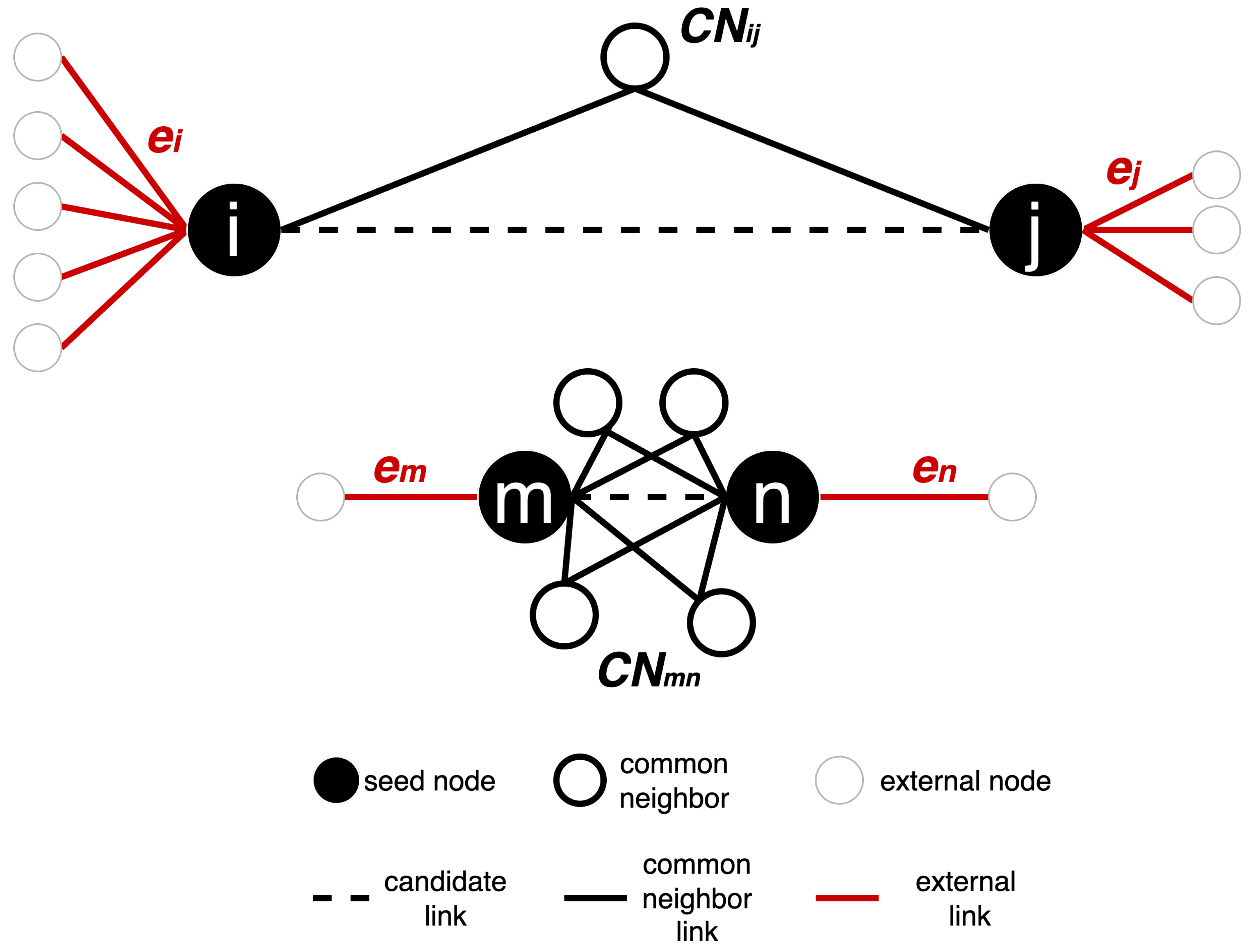
Illustration of how RA measures are computed on two toy networks. Seed nodes are shown in black; common neighbors (CN) are shown in white with a black border, and external nodes are white with a grey border. The dashed line is the edge that is being assigned a weight. External links e denote the number of edges connecting a node to nodes outside its CN set, here in red. In black, the links to common neighbors. For the link in the top network, , , and . For the link in the bottom network, , , and .
Figure A1.
Illustration of how RA measures are computed on two toy networks. Seed nodes are shown in black; common neighbors (CN) are shown in white with a black border, and external nodes are white with a grey border. The dashed line is the edge that is being assigned a weight. External links e denote the number of edges connecting a node to nodes outside its CN set, here in red. In black, the links to common neighbors. For the link in the top network, , , and . For the link in the bottom network, , , and .
Appendix A.1. Latent Geometry-Driven Network Automata rule
Figure A1 illustrates how RA2-based network automata rules assign edge weights by estimating geometric distances using only local topological features. The two toy subnetworks demonstrate how the RA2 rule and its variants distinguish between geometrically distant and close node pairs. In the top subnetwork, nodes i and j have only one common neighbor and are each connected to many external nodes (, ), indicating a weak integration in a local community and stronger connectivity to distinct parts of the network. According to the Repulsion-Attraction rule, this suggests a larger latent distance due to high repulsion and low attraction. In contrast, in the bottom subnetwork, nodes m and n share four common neighbors and have only one external link each (, ). This pattern indicates a stronger local community and a higher likelihood that the nodes are geometrically close in the latent space, with a lower dissimilarity score. These examples highlight how latent geometry-driven RA2-based network automata rules estimate hidden distances: fewer common neighbors and more external links suggest geometrical separation, while many common neighbors and few external links imply proximity in the latent manifold.
Appendix A.2. Time Complexity
We analyze the time complexity for the full dynamic dismantling process (excluding reinsertion) for the latent geometry-driven network automata rules in Table A1, where dynamic means recomputing the dismantling measure after each node removal. For RA2 and its variants, the dominant operation is the computation of the common neighbor (CN) matrix. This operation has a time complexity of for dense graphs and for sparse graphs, where N is the number of nodes and m is the number of links. Assuming N dismantling steps in the worst-case scenario, the overall time complexity becomes for sparse graphs. The assumption of N dismantling steps applies to all the time complexity analyses of dynamic dismantling methods.
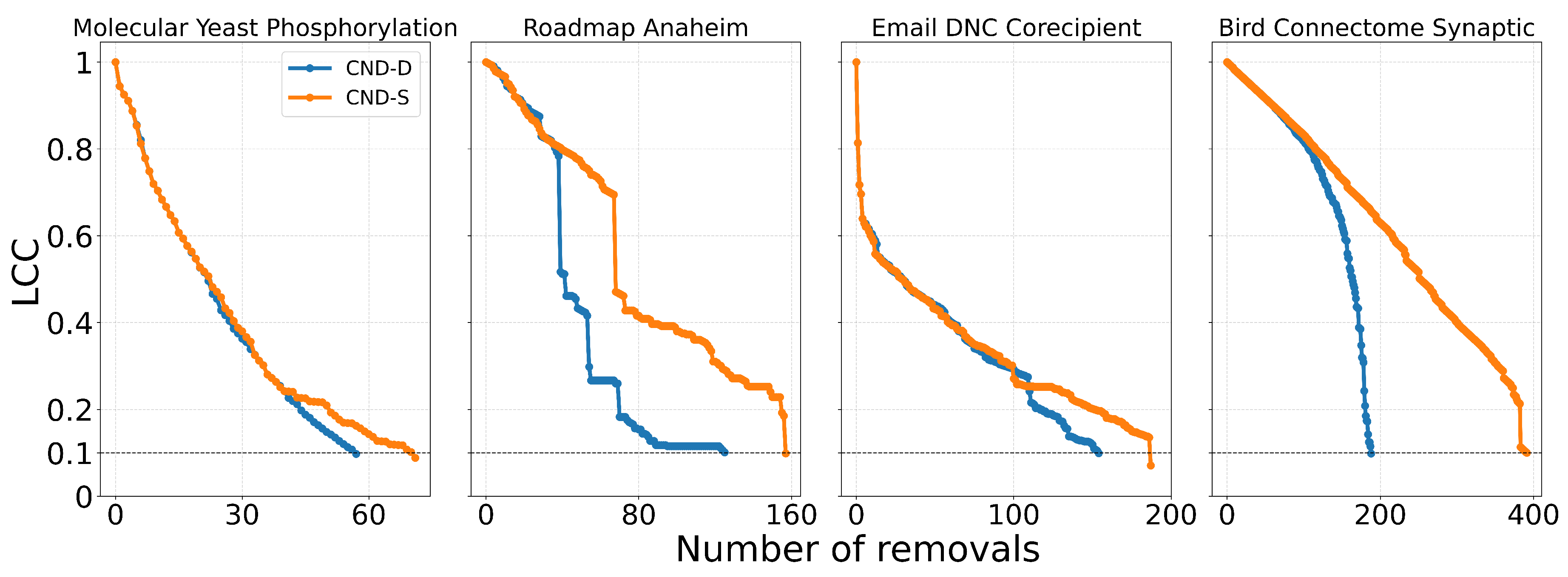
Figure A2.
Dynamic dismantling process on example networks comparing local network automata rule RA2 and its variants versus NBC, when the former outperforms NBC in terms of AUC. The plots show the normalized largest connected component (LCC) versus the number of node removals, with a target LCC threshold of 10%. The final evaluation metric is the Area Under the Curve (AUC) of the LCC trajectory.
Appendix B. Topological Centrality Measures
Table A2.
Comparison of topological centrality measures and the associated time complexity for dynamic dismantling using each centrality measure. Information Locality denotes the type of structural information required to assign a score to each node. Time Complexity denotes the time complexity for dynamic dismantling using each centrality measure on sparse graphs, without reinsertion. N: number of nodes. m: number of links.
| Measure | Author | Year | Type | Information Locality | Time Complexity |
|---|---|---|---|---|---|
| Degree | Degree-based | Local | |||
| Eigenvector | Bonacich [41] | 1972 | Walks-based | Global | |
| Node Betweenness (NBC) | Freeman [24] | 1977 | Shortest path-based | Global | |
| PageRank (PR) | Page et al. [42] | 1999 | Random walk-based | Global | |
| Resilience | Zhang et al. [35] | 2020 | Resilience-based | Global | |
| Domirank | Engsig et al. [25] | 2024 | Fitness-based | Global | |
| Fitness | Servedio et al. [26] | 2025 | Fitness-based | Global |
Appendix B.1. Time Complexity
We analyze the time complexity of dynamic dismantling (excluding reinsertion) for the topological centrality measures used in our experiments, summarized in Table A2. As before, the analysis assumes N dismantling steps in the worst-case scenario. For degree, the score update after each removal is local and can be done in time using a binary heap. For NBC, we use Brandes’ algorithm [52], which computes betweenness centrality in time per step for unweighted networks. Eigenvector, PageRank, Resilience, Domirank, and Fitness all rely on matrix-vector multiplications, which has a time complexity of . We also add the term N, which represents the overhead of looping over nodes to update or normalize the resulting vector at each iteration. This leads to a total per-step cost of . We also omit the constant k for Eigenvector, PageRank, and Fitness centrality, which represents the number of iterations these methods perform. In practice, reaching full convergence to a single optimal solution is often computationally infeasible; this is why a fixed number of k iterations is typically defined.
Appendix C. Statistical and Machine Learning Network Dismantling
Table A3.
Comparison of dismantling algorithms [6]. Information Locality denotes the type of structural information required to assign a score to each node. Dynamicity indicates whether scores are recomputed after each removal. Reinsertion specifies whether the algorithm includes a reinsertion step after dismantling. Time Complexity denotes the time complexity of the method on sparse graphs, without reinsertion. N: number of nodes. m: number of links. h: number of attention heads. T: maximal diameter of the trees in the forest for BPD and MS. is a small constant used in spectral partitioning operations. Included states whether the method was run in our experiments; if not, a brief reason is provided.
| Algorithm | Type | Author | Year | Information Locality | Dynamicity | Reinsertion | Time Complexity | Included |
|---|---|---|---|---|---|---|---|---|
| Collective Influence (CI) | Influence maximization | Morone et al. [3] | 2016 | Local | Dynamic | Yes | Yes | |
| Belief propagation-guided decimation (BPD) | Message passing-based decycling | Mugisha & Zhou [4] | 2016 | Global | Dynamic | Optional | No - Code missing | |
| Min-Sum (MS) | Message passing-based decycling | Braunstein et al. [2] | 2016 | Global | Dynamic | Yes | Yes | |
| Generalized Network Dismantling (GND) | Spectral partitioning | Ren et al. [34] | 2019 | Global | Dynamic | Optional | Yes | |
| CoreHD | Degree-based decycling | Zdeborová et al. [32] | 2016 | Global | Dynamic | Yes | Yes | |
| Explosive Immunization (EI) | Explosive percolation | Clusella et al. [33] | 2016 | Global | Dynamic | No | Yes | |
| FINDER | Machine learning | Fan et al. [43] | 2020 | Global | Dynamic | Optional | No - Code outdated | |
| Graph Dismantling Machine (GDM) | Machine learning | Grassia et al. [36] | 2021 | Global | Static | Optional | Yes | |
| CoreGDM | Machine learning | Grassia & Mangioni [37] | 2023 | Global | Static | Yes | Yes |
Table A3 is adapted and extended from Table 1 of Artime et al. [6], a recent and comprehensive review which has become a key reference in the field of network dismantling. The majority of these algorithms were included in our experiments, with the exception of BPD and FINDER due to unavailable or outdated code, respectively.
Figure A3.
Mean field ranking for a subset of the best-performing methods from each category with each reinsertion method (R1, R2, R3) (). Methods based on latent geometry are shown in red. All LGD and topological centrality measures use dynamic dismantling. Error bars indicate the standard error of the mean (SEM). Method acronyms are defined in Table A1, Table A2, and Table A3.
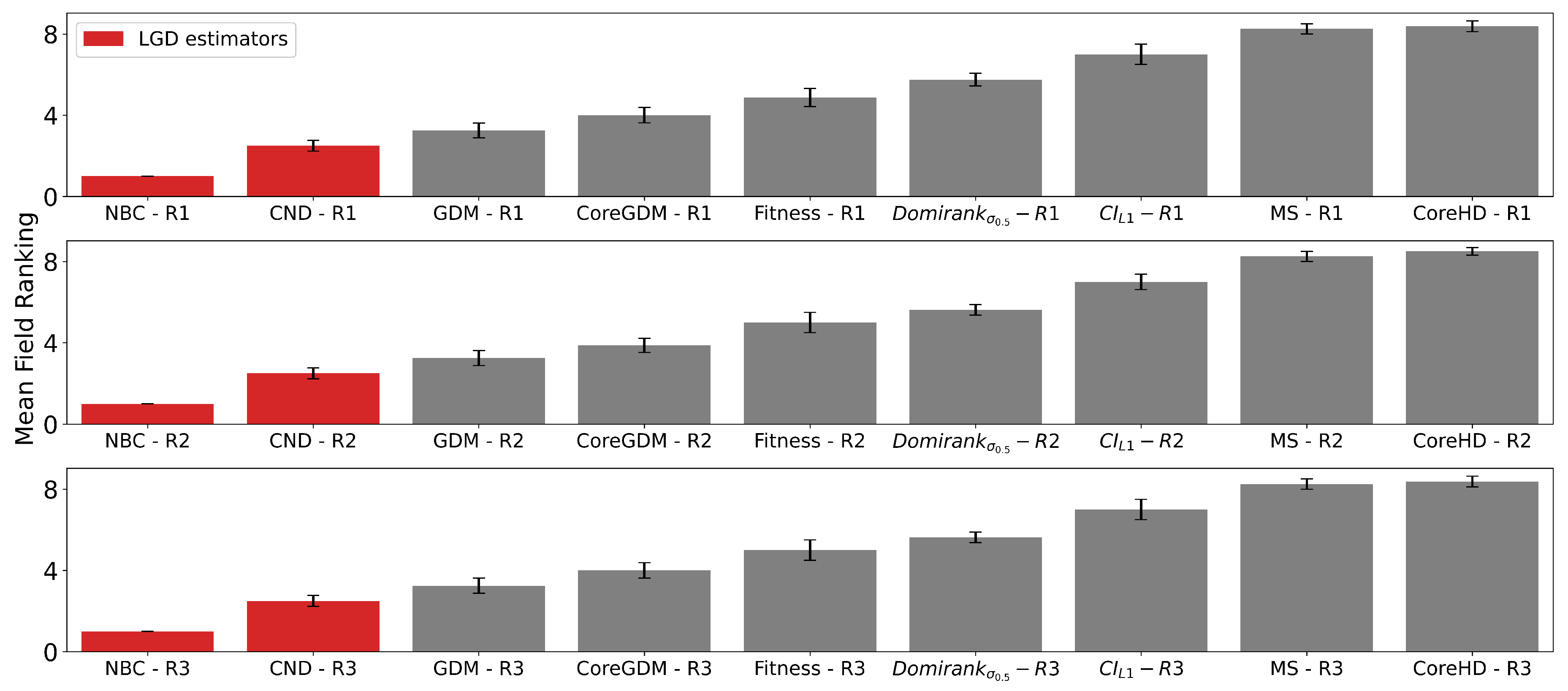
Figure A4.
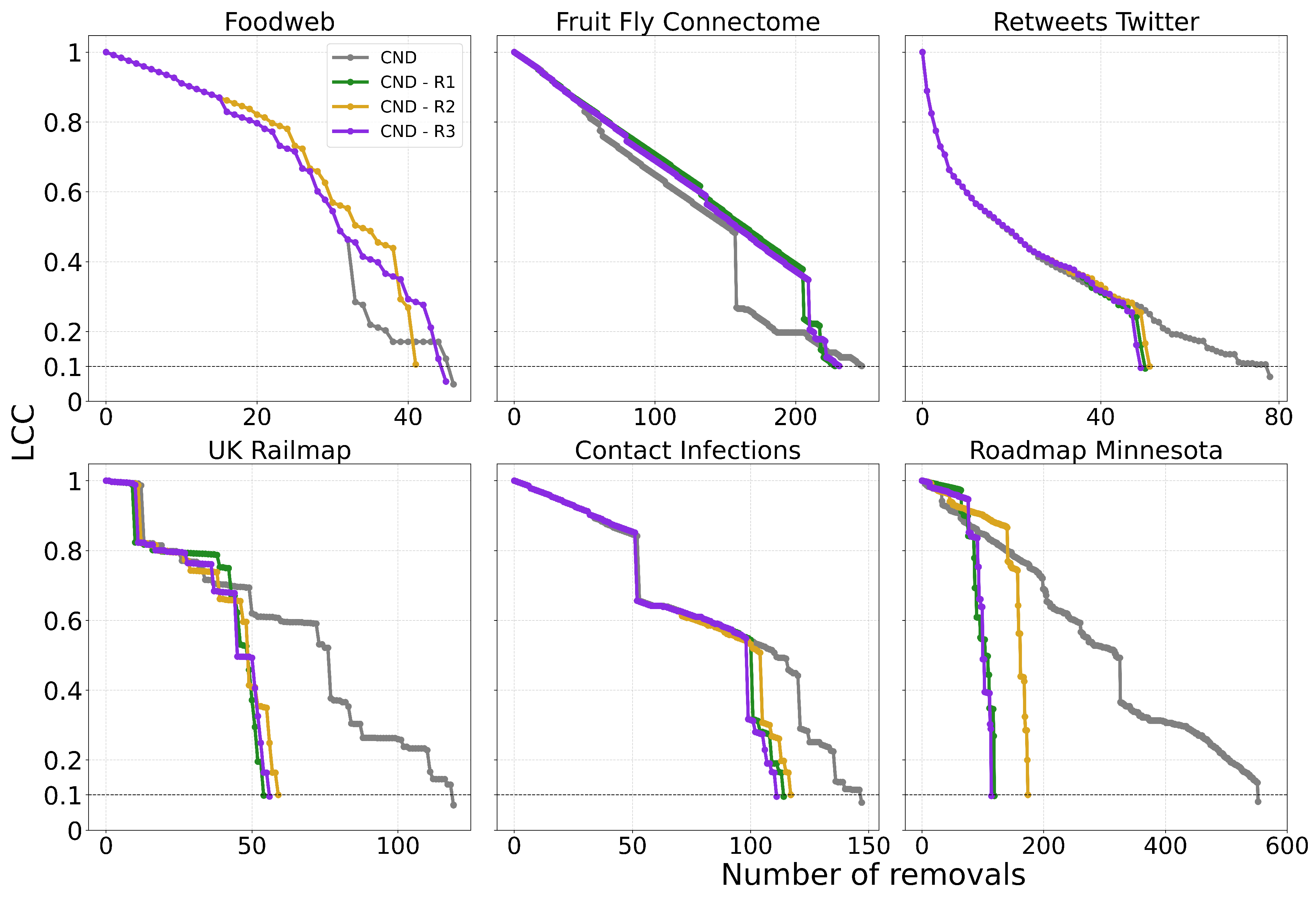
Dynamic dismantling process on example networks comparing CND with and without reinsertion. The plots show the normalized size of the largest connected component (LCC) as a function of the number of node removals, with a target LCC threshold of 10%. The final evaluation metric is the Area Under the Curve (AUC) of the LCC trajectory.
Figure A4.
Dynamic dismantling process on example networks comparing CND with and without reinsertion. The plots show the normalized size of the largest connected component (LCC) as a function of the number of node removals, with a target LCC threshold of 10%. The final evaluation metric is the Area Under the Curve (AUC) of the LCC trajectory.
Appendix D. Reinsertion Methods
Reinsertion was originally introduced in the context of immunization as a reverse process: starting from a fully dismantled network, nodes are reinserted one by one, each time selecting the node whose addition causes the smallest increase in the largest connected component (LCC) [53]. This reversed sequence then defines an effective dismantling order. In subsequent studies, reinsertion has been used as a post-processing step to improve dismantling outcomes [6]: the network is first dismantled by a given method, and nodes are reinserted until the LCC reaches the dismantling threshold. This reduces the number of removed nodes while preserving the original attack target.
Several reinsertion criteria have been proposed: Braunstein et al. [2] select the node that ends up in the smallest resulting component after reinsertion; Morone et al. [3] choose the node that reconnects the fewest components; Mugisha and Zhou [4] select the node that causes the smallest LCC increase. See Table A4 for a full comparison.
Reinsertion can greatly enhance dismantling performance. However, recent work shows that this step can overpower the dismantling algorithm itself, allowing weak methods to appear effective when paired with reinsertion [45]. To address this, we enforce two constraints to ensure fair comparisons and prevent reinsertion from dominating the dismantling process:
- Reinsertion must stop once the LCC exceeds the dismantling threshold. Recomputing a new dismantling order by reinserting all nodes is not allowed.
- Ties in the reinsertion criterion must be broken by reversing the dismantling order: nodes removed later are prioritized.
These rules ensure that reinsertion complements rather than overrides the dismantling process, preserving the integrity of the original method.
In our experiments, we implement three reinsertion methods, adapted from prior work, here we explain which part of their method we change for our experiments. Those changes are marked with an asterisk (*) in Table A4.:
- R1 (Braunstein et al.) [2]: We replace their original tiebreak (smallest node index) with reverse dismantling order.
- R2 (Morone et al.) [3]: We apply the LCC stopping condition. Originally, all nodes are reinserted to compute a new dismantling sequence.
- R3 (Mugisha & Zhou) [4]: We apply reverse dismantling order as the tiebreak, as no rule is defined in their paper, and their code is unavailable.
R3 is the most similar to the reverse immunization method proposed by Schneider et al. (2012) [53], where nodes are added back one by one based on minimal LCC growth. In their original method, ties are broken by selecting the node with the fewest connections to already reinserted nodes; if multiple candidates remain, one is chosen at random.
We note that reinsertion typically reduces the number of removals but does not always lead to a lower AUC. Since the trajectory of the LCC changes with reinsertion, the dismantling process may reach the threshold faster, improving AUC. However, this is not guaranteed, as we see in the first two subplots of Figure A4 for the Foodweb and Fruit Fly Connectome networks. The methods with reinsertion arrive at the dismantling threshold in fewer number of removals, but the change in the LCC curve results in a worse final AUC.
We also see that the reduction in AUC is not proportional to the reduction in the number of removals, as seen in Figure A5 for CND. Indeed, reinsertion, by definition, reinserts nodes that were ultimately unnecessary for the dismantling process to reach its target.
Appendix D.1. Time Complexity
We report the total time complexity of each reinsertion method over the full reinsertion process in Table A4, assuming all dismantled nodes are considered for reinsertion for every step and that all nodes are reinserted. Candidates for reinsertion are denoted as r. A a result, we multiply the per-step cost of updating for each method by the total number of reinsertion candidates. is the maximum number of components a node can connect to, equal to the maximum degree in the original graph, and is the maximum size of any connected component during the reinsertion phase. For R1, the candidate node that ends up in the smallest resulting component is selected. Reinserting a node may merge up to components, each of size at most , requiring an update of at most nodes. These updates are tracked in a binary heap of size r, where at maximum nodes have to be updated, giving a cost of per update. The per-step cost is therefore . R2 selects the node that connects the fewest existing components. Unlike R1, it requires inspecting not only the components merged by the candidate node, but also the neighbors of the affected neighbors. This increases the complexity by a factor of , resulting in a per-step time complexity of . R3 evaluates each candidate by explicitly computing the resulting LCC size after reinsertion. Each evaluation requires a graph traversal to recompute connected components, which takes time on sparse graphs. This has to be done for each reinsertion candidate, at every step, so ,
Table A4.
Comparison of reinsertion methods. Criteria defines the criterion for selecting which node to reinsert. Tiebreak specifies how ties are resolved. LCC Condition indicates whether all dismantled nodes are reinserted or if reinsertion stops once the predefined LCC threshold is reached. Time Complexity denotes the time complexity of each reinsertion method on sparse graphs, for the whole reinsertion process. N: number of nodes. m: number of links. r: set of reinsertion candidates. : maximum degree in the original graph G. : maximum size of any connected component during the reinsertion phase. Used In lists the methods that use each method, in bold, the dismantling method that originally proposed that reinsertion method. An asterisk (*) marks components of the reinsertion method that were modified in our study, as detailed in Appendix D.
| Name | Author | Year | Criteria | Tiebreak | LCC Condition | Time Complexity | Used In |
|---|---|---|---|---|---|---|---|
| R1 | Braunstein et al. [2] | 2016 | Node that ends up in the smallest component | Reverse dismantling order* | Yes | MS, CoreGDM, CoreHD, GDM, GND | |
| R2 | Morone et al. [3] | 2016 | Node that connects to the fewest clusters | Reverse dismantling order | Yes* | CI | |
| R3 | Mugisha & Zhou [4] | 2016 | Node that causes the smallest increase in LCC size | Reverse dismantling order* | Yes | BPD |
Figure A5.
Mean AUC and number of removals by field for CND without reinsertion and with each reinsertion method (R1, R2, R3) ( for all methods). Error bars represent the standard error of the mean (SEM). Red text indicates the percentage improvement achieved by using the best-performing reinsertion method for each field.
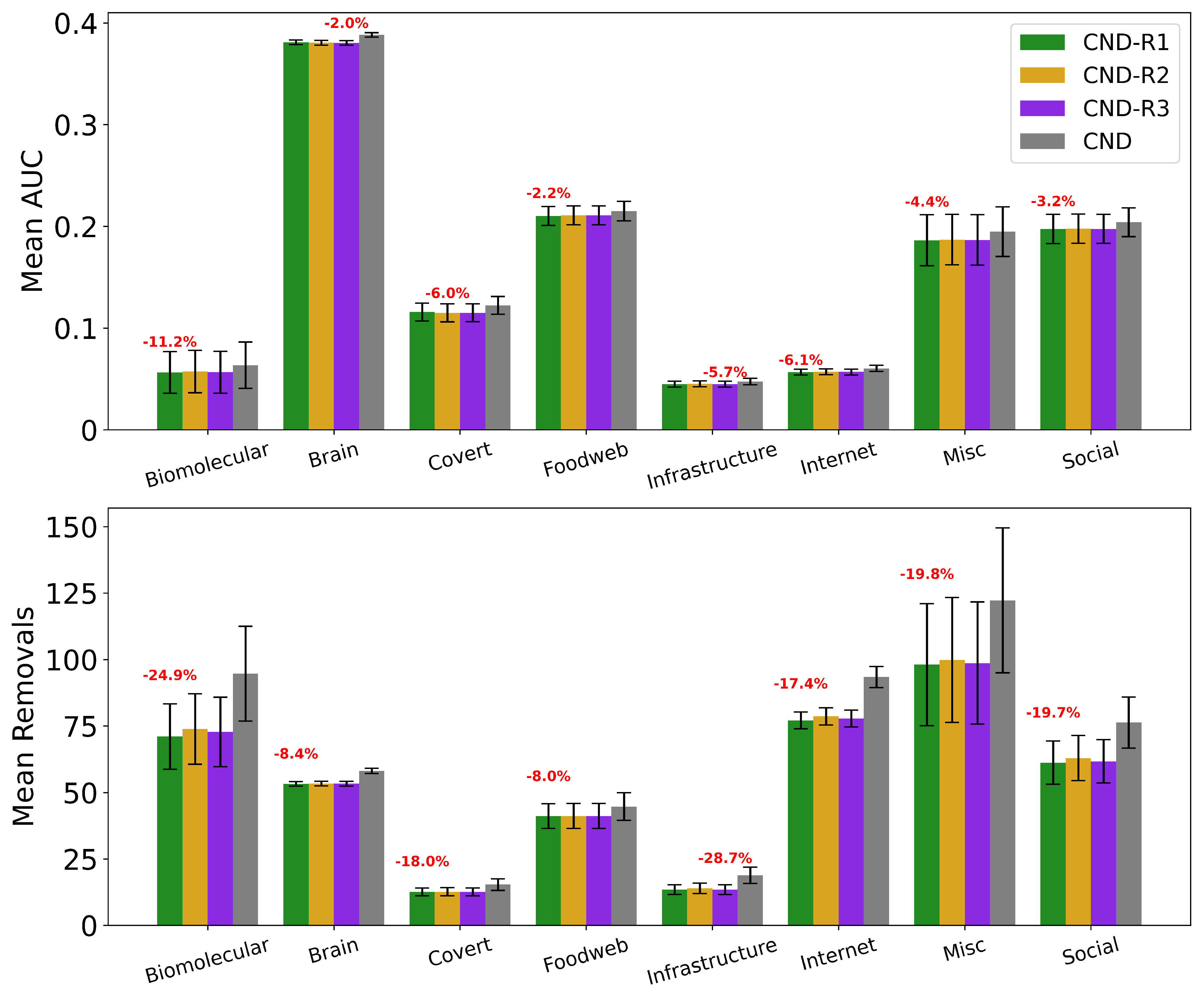
Table A5.
Full summary statistics of the ATLAS networks used in this study, averaged by field: number of subfields and networks, average number of nodes , number of edges , density , mean degree , characteristic path length , assortativity [54], transitivity , mean local clustering coefficient , maximum k-core , average k-core , LCP-corr [55], and modularity [56]
| Field | Biomolecular | Brain | Covert | Foodweb | Infrastructure | Internet | Misc | Social | Total |
|---|---|---|---|---|---|---|---|---|---|
| Subfields | 5 | 1 | 2 | 1 | 7 | 1 | 8 | 7 | 32 |
| Networks | 27 | 529 | 89 | 71 | 314 | 206 | 38 | 201 | 1,475 |
| 2,997 | 97 | 107 | 117 | 664 | 5,708 | 2,880 | 3,267 | ||
| 11,855 | 1,535 | 266 | 1,087 | 1,332 | 19,601 | 19,921 | 53,977 | ||
| 0.01 | 0.34 | 0.17 | 0.16 | 0.07 | 0.01 | 0.07 | 0.11 | ||
| 6.7 | 28.3 | 5.7 | 15.2 | 4.9 | 7.5 | 14.1 | 26.9 | ||
| 4.4 | 1.7 | 3 | 2.2 | 9.9 | 3.4 | 3.5 | 3.5 | ||
| -0.21 | -0.03 | -0.15 | -0.28 | -0.52 | -0.22 | -0.07 | -0.05 | ||
| 0.06 | 0.55 | 0.39 | 0.19 | 0.06 | 0.11 | 0.22 | 0.29 | ||
| 0.13 | 0.63 | 0.46 | 0.22 | 0.11 | 0.31 | 0.34 | 0.36 | ||
| 10.6 | 20.1 | 5.9 | 12.8 | 4.9 | 25 | 21.6 | 25.7 | ||
| 3.6 | 17.5 | 4.2 | 9.2 | 3 | 4 | 8.3 | 15.4 | ||
| 0.66 | 0.97 | 0.76 | 0.67 | 0.15 | 0.94 | 0.85 | 0.77 | ||
| 0.59 | 0.25 | 0.48 | 0.26 | 0.46 | 0.5 | 0.49 | 0.5 |
Table A6.
Number and size of real-world networks tested by dismantling algorithms. N denotes the number of nodes, E the number of edges.
Table A6.
Number and size of real-world networks tested by dismantling algorithms. N denotes the number of nodes, E the number of edges.
| Algorithm | Year | Networks | ||
|---|---|---|---|---|
| Collective Influence (CI) [3] | 2016 | 0 | ||
| CoreHD [32] | 2016 | 12 | 1.7M | 11M |
| Explosive Immunization (EI) [33] | 2016 | 5 | 50K | 344K |
| Min-Sum (MS) [2] | 2016 | 2 | 1.1M | 2.9M |
| Generalized Network Dismantling (GND) [34] | 2019 | 10 | 5K | 17K |
| Resilience Centrality [35] | 2020 | 4 | 1K | 14K |
| Graph Dismantling Machine (GDM) [36] | 2021 | 57 | 1.4M | 2.8M |
| CoreGDM [37] | 2023 | 15 | 79K | 468K |
| Domirank Centrality [25] | 2024 | 6 | 24M | 58M |
| Fitness Centrality [26] | 2025 | 5 | 297 | 4K |
| LGD-NA | 2025 | 1,475 | 23K | 507K |
Appendix E. Dynamic & Static Dismantling
In static dismantling, node scores are computed once at the beginning and are then removed in descending order of importance until the dismantling threshold is reached. In contrast, dynamic dismantling recomputes the scores after each removal. As shown in Figure A6, with CND given as an example, dynamic dismantling consistently outperforms static dismantling across all fields. Dynamic variants achieve lower AUC and fewer removals in every case, confirming the advantage of score recomputation.
Figure A6.
Mean AUC and number of removals for dynamic and static CND (. Error bars represent the standard error of the mean (SEM). Red text indicates the percentage improvement achieved by using dynamic over static variants.
Figure A6.
Mean AUC and number of removals for dynamic and static CND (. Error bars represent the standard error of the mean (SEM). Red text indicates the percentage improvement achieved by using dynamic over static variants.
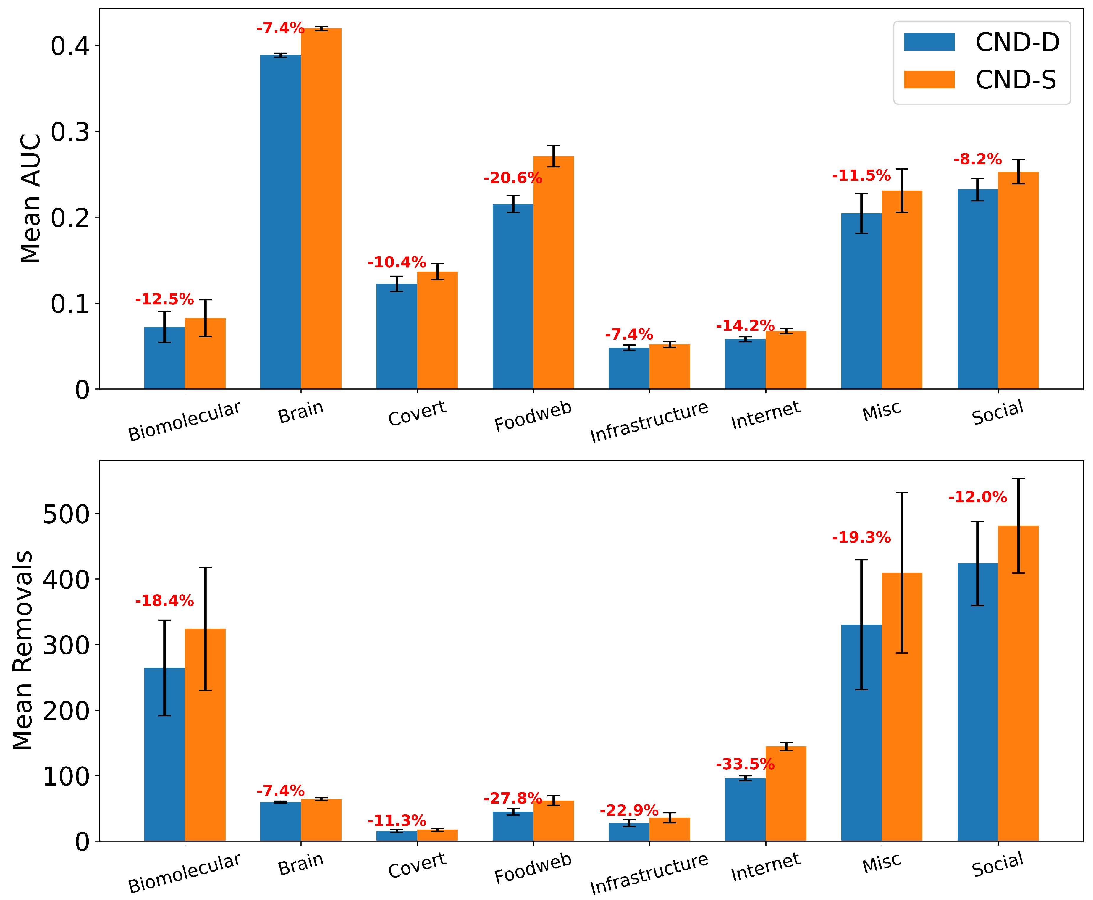
Figure A7.
Dismantling process on example networks comparing dynamic and static CND. The plots show the normalized size of the largest connected component (LCC) as a function of the number of node removals, with a target LCC threshold of 10%. Performance is evaluated using the Area Under the Curve (AUC) of the LCC trajectory.
Appendix F. Experimental Setup
Appendix F.1. Baseline Topological Centrality Measures
We selected centrality measures to cover diverse categories: shortest path-based (NBC), degree-based (degree), walk-based (eigenvector), random walk-based (PageRank), resilience-based (Resilience), and fitness-based (Domirank and Fitness centrality). We also tested closeness and load centrality, but both performed worse than NBC and rely on the same shortest-path principle; thus, we retained NBC. Similarly, Katz centrality underperformed compared to eigenvector centrality and is also based on spectral properties of the adjacency matrix. For DomiRank, we tested three values for the numerator in the parameter formula: 0.1, 0.5, and 0.9. While the original study sometimes performs a grid search to find the optimal per network, this is not feasible for our large-scale evaluation. Instead, we selected a representative range and found that yielded the best performance, and we report that value. The parameter controls the balance between local degree-based dominance and global network-structure-based competition. As , the scores approximate degree centrality. As increases, nodes are evaluated in increasingly competitive environments, where centrality depends more on non-local structural dominance than individual connectivity. For Fitness centrality, we capped the number of iterations at . Without this cap, the method took a prohibitively long time to converge, especially on large networks.
Appendix F.2. Baseline Dismantling Methods
We selected the best-performing and most widely adopted dismantling algorithms from the literature [6]. As mentioned earlier, we did not include BPD and FINDER in our experiments due to unavailable and outdated code, respectively. For Collective Influence (CI), we tested values , where ℓ defines the radius of a ball centered at node i, and is the frontier at distance ℓ (i.e., nodes exactly ℓ hops away). We found that performed best across our benchmarks and report this setting, while performed the worst. For Explosive Immunization (EI), we evaluated both scores and . The score targets high-connectivity nodes to rapidly fragment the network early on. The score aims to prevent large cluster merges near the percolation threshold by avoiding the connection of separate components. We found that consistently outperformed , and thus we use it in our final experiments. For eigenvector centrality, we capped the number of power iterations at to avoid long or unbounded runtimes, since convergence can be very slow in large networks. For PageRank, we used a convergence tolerance of , as the algorithm runs until the change in scores falls below this threshold.
Appendix F.3. Note on Reinsertion
We did not apply reinsertion techniques on all networks included in the initial dismantling experiments. In some cases, certain methods performed so poorly that applying reinsertion became prohibitively slow. To ensure consistency, we excluded these networks from the reinsertion analysis for all methods. Specifically, we imposed a cutoff: networks were excluded if any method required more than 800 node removals to reach the dismantling threshold. Based on this criterion, 59 networks were excluded.
Appendix F.4. Note on Evaluation
A lower number of removals does not always imply a lower AUC. Our AUC metric rewards methods that fragment the network early, even if they require more steps to reach the dismantling threshold. As shown in Figure A8, we show cases where the method reaching the threshold with more removals achieves a lower AUC, due to earlier damage to the network structure.
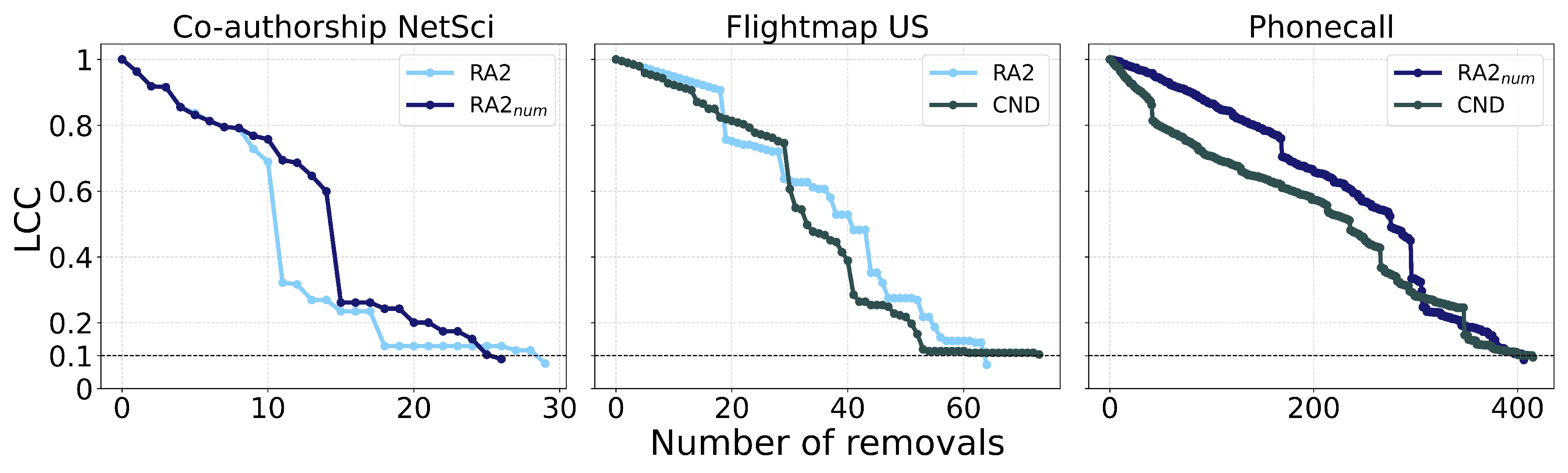
Figure A8.
Dynamic dismantling process on example networks comparing CND, RA2 and , showing a lower removal number does not necessarily mean a lower Area Under the Curve (AUC) of the LCC trajectory. The plots show the normalized size of the largest connected component (LCC) as a function of the number of node removals, with a target LCC threshold of 10%.
Appendix F.5. Code
All our methods are implemented in our codebase, available in the supplementary material. We implement RA2, RA2num, CND, NBC, as well as degree and eigenvector centrality. We also adapt and integrate the original implementations of Domirank centrality and Fitness centrality. Since no code was available for Resilience centrality, we implemented it ourselves based on the original description in the paper. Instructions for running these methods and reproducing the experiments are included in the supplementary material. We also provide a representative network from the ATLAS dataset for testing purposes. For GDM, CoreGDM, GND, CI, EI, MS, and CoreHD, we use the publicly available code from Artime et al. (2024)’s review.
Appendix F.6. Computational Resources
All experiments were conducted on a machine equipped with an AMD Ryzen Threadripper PRO 3995WX CPU (64 cores), 251 GiB of RAM, and a single NVIDIA RTX A4000 GPU with 16 GiB of memory. All code was implemented in Python, with dependencies and library versions specified in the supplementary material to ensure full reproducibility.
Appendix G. Limitations, Future Work, and Broader Impact
Appendix G.1. Limitations
A limitation of this study is the mismatch between theoretical and observed runtimes, which can vary across methods. These differences stem from factors such as the programming language used, hardware acceleration, and implementation-level optimizations. However, all experiments were run on the same CPU and GPU to ensure a fair comparison, and we made a strong effort to optimize all methods both in terms of runtime and dismantling performance. For example, we tested different parameters for Domirank, CI, and EI, and evaluated multiple variants of shortest path-based and spectral partitioning-based centrality measures. Furthermore, we were unable to test on extremely large networks due to hardware constraints and the high computational cost of running a broad set of dismantling methods. However, we are confident that our results would generalize to larger networks, given the diversity of the 1,475 networks tested, spanning a wide range of domains and sizes from very small to large. Another limitation relates to the parameter tuning required by some baseline methods, especially machine learning-based approaches and Domirank. Due to the scale of our experimental setup—both in the number and size of networks—we were unable to perform extensive tuning. Although targeted tuning could enhance performance for specific methods on individual networks, it would compromise consistency across the wide range of complex systems domains considered. In contrast, LGD-NA requires no parameter tuning and consistently achieves strong, generalizable performance across all tested networks.
Appendix G.2. Future Work
Future research could further explore latent geometry, particularly how to effectively combine local and global information in dismantling strategies. Improving the scalability of matrix-based computations, especially for very large and sparse networks, is another important direction. There is also a need for more cost-efficient dynamic dismantling strategies that reduce the overhead of recomputing scores after every node removal without significantly sacrificing performance. In addition, edge dismantling remains a relatively underexplored area compared to node-based dismantling, and it would be valuable to investigate whether latent geometry-driven principles can also guide the efficient removal of links in complex networks. Targeting edges can be just as important as targeting nodes, and in many real-world systems, such as transportation networks (railroads, roads, subways, or shipping trade routes), edge removal may represent the more realistic and sensible threat scenario, making it highly relevant for dismantling strategies.
Appendix G.3. Broader Impact
Understanding and improving network dismantling has direct applications in fields such as epidemiology, infrastructure protection, and information control. While dismantling techniques could theoretically be misused to disrupt critical systems, they also play a crucial role in strengthening the robustness of real-world networks against attacks or failures. By publishing this work openly—including the theoretical foundations, code, and extensive evaluation—we aim to ensure transparency and reproducibility. We believe the benefits of improving defensive strategies and system robustness outweigh the potential for misuse.
References
- Alessandro Muscoloni, Josephine Maria Thomas, Sara Ciucci, Ginestra Bianconi, and Carlo Vittorio Cannistraci. Machine learning meets complex networks via coalescent embedding in the hyperbolic space. Nature Communications, 8(1), 2017.
- Alfredo Braunstein, Luca Dall’Asta, Guilhem Semerjian, and Lenka Zdeborová. Network dismantling. Proceedings of the National Academy of Sciences, 113(44):12368–12373, 2016.
- Flaviano Morone, Byungjoon Min, Lin Bo, Romain Mari, and Hernán A. Makse. Collective influence algorithm to find influencers via optimal percolation in massively large social media. Scientific Reports, 6(1), 2016.
- Salomon Mugisha and Hai-Jun Zhou. Identifying optimal targets of network attack by belief propagation. Phys. Rev. E, 94:012305, Jul 2016.
- M. E. J. Newman. The structure and function of complex networks. SIAM Review, 45(2):167–256, 2003.
- Oriol Artime, Marco Grassia, Manlio De Domenico, James P. Gleeson, Hernán A. Makse, Giuseppe Mangioni, Matjaž Perc, and Filippo Radicchi. Robustness and resilience of complex networks. Nature Reviews Physics, 6(2), 2024.
- Réka Albert, Hawoong Jeong, and Albert-László Barabási. Error and attack tolerance of complex networks. Nature, 406(6794):378–382, Jul 2000.
- Albert-László Barabási and Réka Albert. Emergence of scaling in random networks. Science, 286(5439):509–512, 1999.
- Anna D. Broido and Aaron Clauset. Scale-free networks are rare. Nature Communications, 10(1):1017, Mar 2019.
- Ivan Voitalov, Pim van der Hoorn, Remco van der Hofstad, and Dmitri Krioukov. Scale-free networks well done. Phys. Rev. Res., 1:033034, Oct 2019.
- Matteo Serafino, Giulio Cimini, Amos Maritan, Andrea Rinaldo, Samir Suweis, Jayanth R. Banavar, and Guido Caldarelli. True scale-free networks hidden by finite size effects. Proceedings of the National Academy of Sciences, 118(2):e2013825118, 2021.
- M. E. J. Newman. Communities, modules and large-scale structure in networks. Nature Physics, 8(1):25–31, Jan 2012.
- Santo Fortunato and Mark E. J. Newman. 20 years of network community detection. Nature Physics, 18(8):848–850, Aug 2022.
- Erzsébet Ravasz and Albert-László Barabási. Hierarchical organization in complex networks. Phys. Rev. E, 67:026112, Feb 2003.
- Aaron Clauset, Cristopher Moore, and M. E. J. Newman. Hierarchical structure and the prediction of missing links in networks. Nature, 453(7191):98–101, May 2008.
- Federico Battiston, Enrico Amico, Alain Barrat, Ginestra Bianconi, Guilherme Ferraz de Arruda, Benedetta Franceschiello, Iacopo Iacopini, Sonia Kéfi, Vito Latora, Yamir Moreno, Micah M. Murray, Tiago P. Peixoto, Francesco Vaccarino, and Giovanni Petri. The physics of higher-order interactions in complex systems. Nature Physics, 17(10):1093–1098, Oct 2021.
- Renaud Lambiotte, Martin Rosvall, and Ingo Scholtes. From networks to optimal higher-order models of complex systems. Nature Physics, 15(4):313–320, Apr 2019.
- Zhihao Wu, Giulia Menichetti, Christoph Rahmede, and Ginestra Bianconi. Emergent complex network geometry. Scientific Reports, 5(1):10073, May 2015.
- Marián Boguñá, Ivan Bonamassa, Manlio De Domenico, Shlomo Havlin, Dmitri Krioukov, and M. Ángeles Serrano. Network geometry. Nature Reviews Physics, 3(2), 2021.
- Dmitri Krioukov, Fragkiskos Papadopoulos, Maksim Kitsak, Amin Vahdat, and Marián Boguñá. Hyperbolic geometry of complex networks. Phys. Rev. E, 82:036106, Sep 2010.
- M. Ángeles Serrano, Dmitri Krioukov, and Marián Boguñá. Self-similarity of complex networks and hidden metric spaces. Phys. Rev. Lett., 100:078701, Feb 2008.
- Dirk Brockmann and Dirk Helbing. The hidden geometry of complex, network-driven contagion phenomena. Science, 342(6164):1337–1342, 2013.
- Muscoloni Alessandro and Cannistraci Carlo Vittorio. Leveraging the nonuniform pso network model as a benchmark for performance evaluation in community detection and link prediction. New Journal of Physics, 20(6):063022, jun 2018.
- Linton C. Freeman. A set of measures of centrality based on betweenness. Sociometry, 40(1):35–41, 1977.
- Marcus Engsig, Alejandro Tejedor, Yamir Moreno, Efi Foufoula-Georgiou, and Chaouki Kasmi. Domirank centrality reveals structural fragility of complex networks via node dominance. Nature Communications, 15(1):56, Jan 2024.
- Vito D P Servedio, Alessandro Bellina, Emanuele Calò, and Giordano De Marzo. Fitness centrality: a non-linear centrality measure for complex networks. Journal of Physics: Complexity, 6(1):015002, jan 2025.
- Adilson E. Motter and Ying-Cheng Lai. Cascade-based attacks on complex networks. Phys. Rev. E, 66:065102, Dec 2002.
- Petter Holme, Beom Jun Kim, Chang No Yoon, and Seung Kee Han. Attack vulnerability of complex networks. Phys. Rev. E, 65:056109, May 2002.
- Marián Boguñá, Dmitri Krioukov, and K. C. Claffy. Navigability of complex networks. Nature Physics, 5(1), 2009.
- Jon M. Kleinberg. Navigation in a small world. Nature, 406(6798), 2000.
- Alessandro Muscoloni and Carlo Vittorio Cannistraci. Navigability evaluation of complex networks by greedy routing efficiency. Proceedings of the National Academy of Sciences, 116(5):1468–1469, 2019.
- Lenka Zdeborová, Pan Zhang, and Hai-Jun Zhou. Fast and simple decycling and dismantling of networks. Scientific Reports, 6(1), 2016.
- Pau Clusella, Peter Grassberger, Francisco J. Pérez-Reche, and Antonio Politi. Immunization and targeted destruction of networks using explosive percolation. Phys. Rev. Lett., 117:208301, Nov 2016.
- Xiao-Long Ren, Niels Gleinig, Dirk Helbing, and Nino Antulov-Fantulin. Generalized network dismantling. Proceedings of the National Academy of Sciences, 116(14):6554–6559, 2019.
- Yongtao Zhang, Cunqi Shao, Shibo He, and Jianxi Gao. Resilience centrality in complex networks. Phys. Rev. E, 101:022304, Feb 2020.
- Marco Grassia, Manlio De Domenico, and Giuseppe Mangioni. Machine learning dismantling and early-warning signals of disintegration in complex systems. Nature Communications, 12(1), 2021.
- Marco Grassia and Giuseppe Mangioni. Coregdm: Geometric deep learning network decycling and dismantling. In Andreia Sofia Teixeira, Federico Botta, José Fernando Mendes, Ronaldo Menezes, and Giuseppe Mangioni, editors, Complex Networks XIV, pages 86–94, Cham, 2023. Springer Nature Switzerland.
- Konstantin Zuev, Marián Boguñá, Ginestra Bianconi, and Dmitri Krioukov. Emergence of soft communities from geometric preferential attachment. Scientific Reports, 5(1):9421, Apr 2015.
- Alessandro Muscoloni and Carlo Vittorio Cannistraci. A nonuniform popularity-similarity optimization (npso) model to efficiently generate realistic complex networks with communities. New Journal of Physics, 20(5):052002, may 2018.
- Fragkiskos Papadopoulos, Maksim Kitsak, M. Ángeles Serrano, Marián Boguñá, and Dmitri Krioukov. Popularity versus similarity in growing networks. Nature, 489(7417):537–540, Sep 2012.
- Phillip Bonacich and. Factoring and weighting approaches to status scores and clique identification. The Journal of Mathematical Sociology, 2(1):113–120, 1972.
- Lawrence Page, Sergey Brin, Rajeev Motwani, and Terry Winograd. The pagerank citation ranking: Bringing order to the web. Technical Report 1999-66, Stanford InfoLab, November 1999. Previous number = SIDL-WP-1999-0120.
- Changjun Fan, Li Zeng, Yizhou Sun, and Yang-Yu Liu. Finding key players in complex networks through deep reinforcement learning. Nature Machine Intelligence, 2(6):317–324, Jun 2020.
- Ginestra Bianconi, Richard K. Darst, Jacopo Iacovacci, and Santo Fortunato. Triadic closure as a basic generating mechanism of communities in complex networks. Phys. Rev. E, 90:042806, Oct 2014.
- Changjun Fan, Li Zeng, Yanghe Feng, Baoxin Xiu, Jincai Huang, and Zhong Liu. Revisiting the power of reinsertion for optimal targets of network attack. Journal of Cloud Computing, 9(1), 2020.
- Rui Fan, Ke Xu, and Jichang Zhao. A gpu-based solution for fast calculation of the betweenness centrality in large weighted networks. PeerJ Computer Science, 3:e140, 2017.
- Zhiao Shi and Bing Zhang. Fast network centrality analysis using gpus. BMC Bioinformatics, 12(1):149, May 2011.
- Prasanna Pande and David A. Bader. Computing betweenness centrality for small world networks on a gpu. In Proceedings of the 15th Annual High Performance Embedded Computing Workshop (HPEC), September 2011.
- Adam McLaughlin and David A. Bader. Accelerating gpu betweenness centrality. Commun. ACM, 61(8):85–92, July 2018.
- Ahmet Erdem Sariyüce, Kamer Kaya, Erik Saule, and Ümit V. Çatalyürek. Betweenness centrality on gpus and heterogeneous architectures. In Proceedings of the 6th Workshop on General Purpose Processor Using Graphics Processing Units, GPGPU-6, page 76–85, New York, NY, USA, 2013. Association for Computing Machinery.
- Massimo Bernaschi, Giancarlo Carbone, and Flavio Vella. Scalable betweenness centrality on multi-gpu systems. In Proceedings of the ACM International Conference on Computing Frontiers, CF ’16, page 29–36, New York, NY, USA, 2016. Association for Computing Machinery.
- Ulrik Brandes and. A faster algorithm for betweenness centrality*. The Journal of Mathematical Sociology, 25(2):163–177, 2001.
- C. M. Schneider, T. Mihaljev, and H. J. Herrmann. Inverse targeting —an effective immunization strategy. Europhysics Letters, 98(4):46002, may 2012.
- M. E. J. Newman. Assortative mixing in networks. Phys. Rev. Lett., 89:208701, Oct 2002.
- Carlo Vittorio Cannistraci, Gregorio Alanis-Lobato, and Timothy Ravasi. From link-prediction in brain connectomes and protein interactomes to the local-community-paradigm in complex networks. Scientific Reports, 3(1):1613, Apr 2013.
- M. E. J. Newman. Detecting community structure in networks. The European Physical Journal B, 38(2):321–330, Mar 2004.
Figure 1.
Overview of the LGD Network Automata framework. A: Begin with an unweighted and undirected network. B: Estimate latent geometry by assigning a weight to each edge between nodes i and j using local latent geometry estimators (see Table A1). C: Construct a dissimilarity-weighted network based on these weights. D: Compute node strength as the sum of geometric weights to all neighbors in :E–F: Perform dynamic dismantling by iteratively computing node strengths, removing the node with the highest and its edges, and checking whether the normalized size of the largest connected component (LCC) has dropped below a threshold. G–H (optional): Reinsert dismantled nodes using a selected reinsertion method (see Table A4).
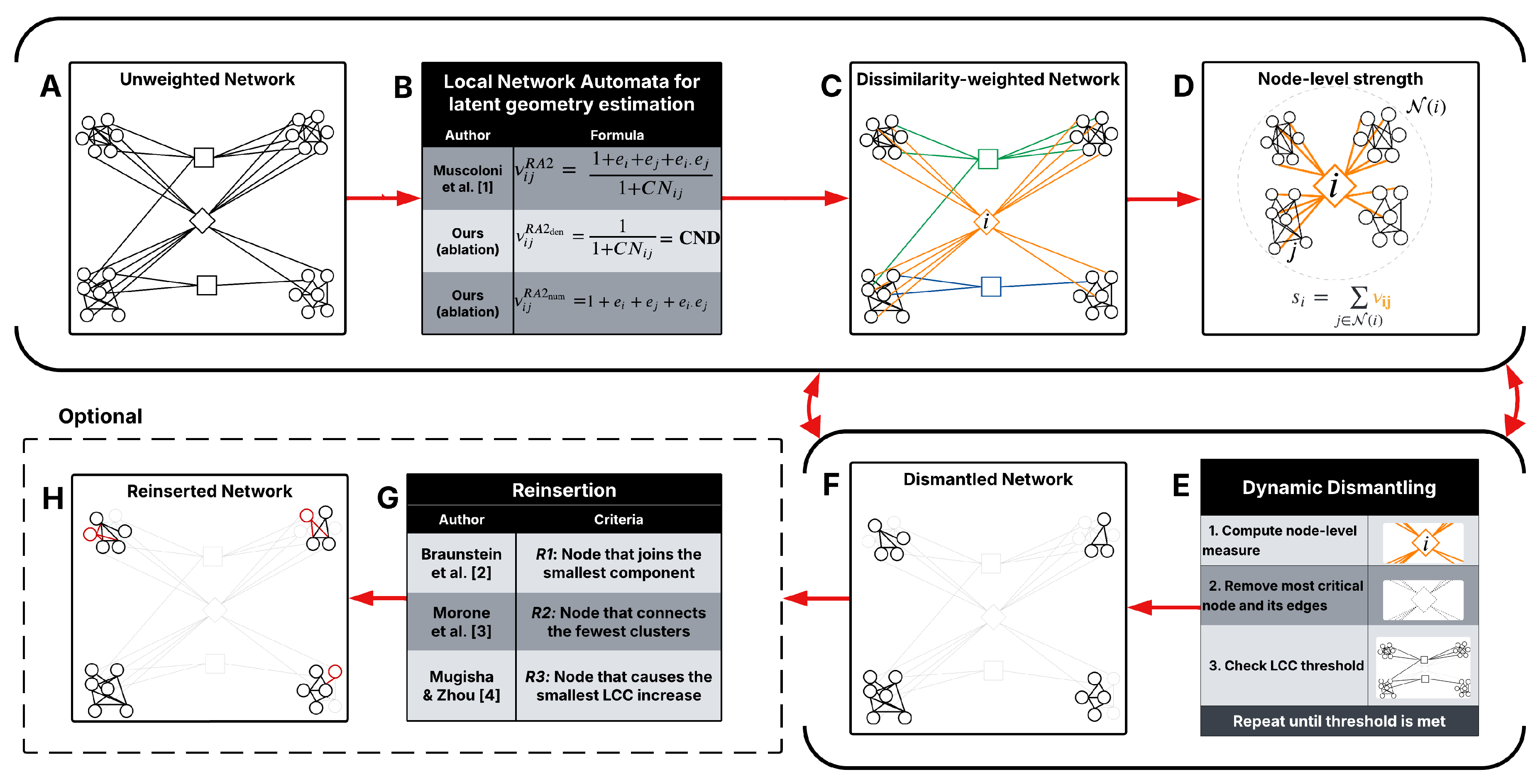
Figure 2.
Mean field ranking for each dismantling method without reinsertion (; upper panel) and with reinsertion (; lower panel). NBC is a global topology LGD estimator. CND, RA2, and are local topology LGD estimators based on network automata rules. All other methods are described in Section 2 and Appendix . In the lower panel, a subset of the best-performing methods from each category is paired with their respective best-performing reinsertion strategy (R1, R2, or R3), see Table A4. Methods based on latent geometry are shown in red. All LGD and topological centrality measures use dynamic dismantling. For EI, CI, and Domirank, we report results with their optimal parameter configurations. denotes variants where the original reinsertion step was disabled. Error bars indicate the standard error of the mean (SEM). Method acronyms are defined in Table A1, Table A2, and Table A3.
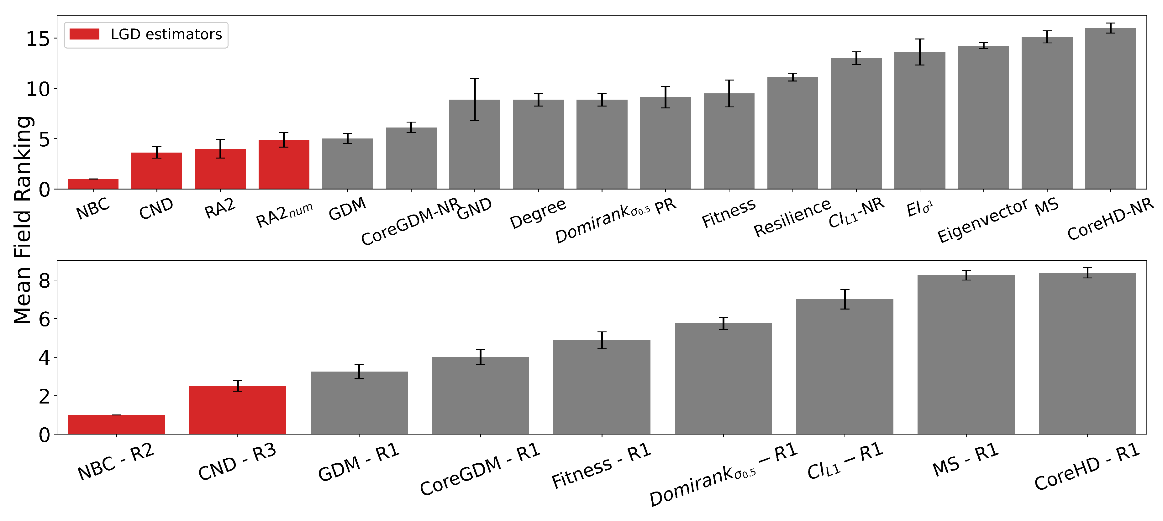
Figure 3.
Runtime (in hours) is plotted against network size, measured by the number of edges, E, for dynamic dismantling. The annotated time indicates the runtime for the largest network. The GPU implementation of NBC did not yield speedup, as discussed in Section 4.5. Evaluated on networks of up to 23,000 nodes and 507,000 edges ().
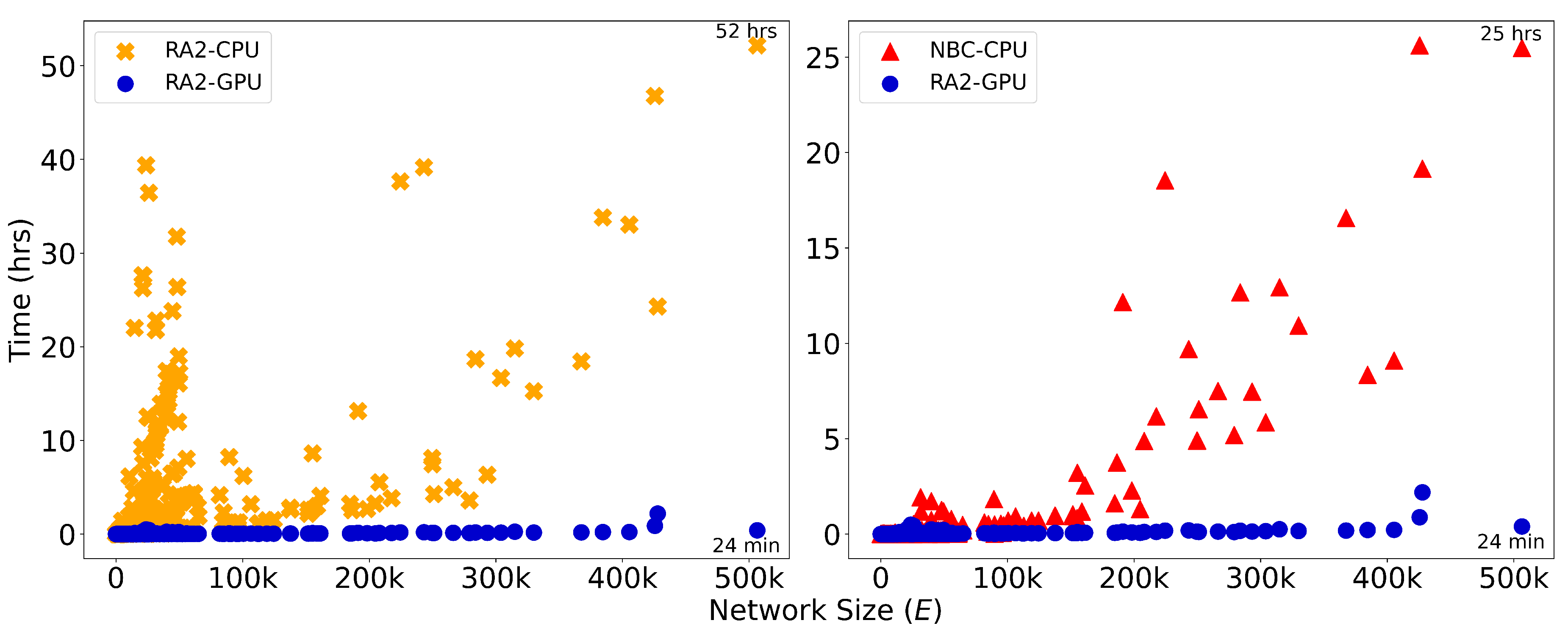
Table 1.
Number of real-world networks tested by dismantling algorithms, see Table A6 for more information.
Table 1.
Number of real-world networks tested by dismantling algorithms, see Table A6 for more information.
| Algorithm | Year | Networks | Ref. |
|---|---|---|---|
| Collective Influence (CI) | 2016 | 0 | [3] |
| CoreHD | 2016 | 12 | [32] |
| Explosive Immunization (EI) | 2016 | 5 | [33] |
| Min-Sum (MS) | 2016 | 2 | [2] |
| GND | 2019 | 10 | [34] |
| Resilience Centrality | 2020 | 4 | [35] |
| GDM | 2021 | 57 | [36] |
| CoreGDM | 2023 | 15 | [37] |
| Domirank Centrality | 2024 | 6 | [25] |
| Fitness Centrality | 2025 | 5 | [26] |
| LGD-NA | 2025 | 1,475 | Ours |
Table 2.
Summary of real-world networks tested in this paper, see Table A5 for more information.
Table 2.
Summary of real-world networks tested in this paper, see Table A5 for more information.
| Field | Subfields | Types | Networks |
|---|---|---|---|
| Biomolecular | 5 | PPI, Genetic, Metabolic, Molecular, Transcription | 27 |
| Brain | 1 | Connectome | 529 |
| Covert | 2 | Covert, Terrorist | 89 |
| Foodweb | 1 | Foodweb | 71 |
| Infrastructure | 7 | Flight, Nautical, Power grid, Rail, Road, Subway, Trade | 314 |
| Internet | 1 | Internet | 206 |
| Misc | 8 | Citation, Copurchasing, Game, Hiring, Lexical, Phone call, Software, Vote | 38 |
| Social | 7 | Coauthorship, Collaboration, Contact, Email, Friendship, Social network, Trust | 201 |
| Total | 32 | 1,475 |
Disclaimer/Publisher’s Note: The statements, opinions and data contained in all publications are solely those of the individual author(s) and contributor(s) and not of MDPI and/or the editor(s). MDPI and/or the editor(s) disclaim responsibility for any injury to people or property resulting from any ideas, methods, instructions or products referred to in the content. |
© 2025 by the authors. Licensee MDPI, Basel, Switzerland. This article is an open access article distributed under the terms and conditions of the Creative Commons Attribution (CC BY) license (http://creativecommons.org/licenses/by/4.0/).
Copyright: This open access article is published under a Creative Commons CC BY 4.0 license, which permit the free download, distribution, and reuse, provided that the author and preprint are cited in any reuse.


