On the Definition of Velocity and the Geometry of Special Relativity

Philip Richard Asquith

doi:10.20944/preprints202505.2272.v2

Submitted:

31 May 2025

Posted:

04 June 2025

You are already at the latest version

Abstract

This article uses the Symmetrical Reflected Radar Model (SRRM) that was described in viXra 2504.0064 to analyse special relativity. The SRRM was developed without making any assumptions about the definition of velocity so that the fundamental relationship between distance and time could be clearly identified. In the SRRM, the algebra of special relativity is reliably represented in a symmetrical spacetime diagram. The transformation equations and geometry of the SRRM describe two symmetrical orthogonal coordinate systems rotating as mirror images; one clockwise, the other anticlockwise, as relative velocity changes. In a transformation between the two symmetrical orthogonal coordinate systems of the SRRM, the spacetime interval is invariant using Pythagoras. It is concluded that, in a symmetrical model, spacetime in special relativity is Euclidian. The terms and equations of the SRRM are shown to be completely interchangeable with those of the generally used Lorenz Transformation. There is good evidence to conclude that the velocity term used in the SRRM is fundamental. Thus, the velocity term used in the Lorenz Transformation is an approximation to the fundamental definition of velocity. Almost all derivations of the Lorenz Transformation since special relativity was first described have been made after first assuming the definition of velocity. This unstated assumption has thus been a silent axiom of the theory, inherent in subsequent analysis, inevitably affecting the conclusions of the theory.

Keywords:

Special relativity

;

Euclidian geometry

;

Loedel diagram

;

Minkowski diagram

;

Lorenz Transformation

;

Velocity

;

Spacetime

Subject:

Physical Sciences - Mathematical Physics

Introduction

This article uses the Symmetrical Reflected Radar Model (SRRM) [1,2] to analyse special relativity.

The SRRM was developed without making any assumptions about the definition of velocity so that the fundamental relationship between distance and time could be clearly identified.

Firstly, it will be shown that the terms and equations of the SRRM are completely interchangeable with those of the generally used Lorenz Transformation (LT).

In developing the SRRM, the algebra of special relativity has been reliably represented in a symmetrical spacetime diagram. It will be shown that the transformation equations of the SRRM describe two Symmetrical Orthogonal Coordinate Systems (SOCS) rotating as mirror images; one clockwise, the other anticlockwise, as relative velocity changes.

In a transformation between the two SOCS of the SRRM, the spacetime interval is invariant using Pythagoras. It is concluded that, in a symmetrical model, spacetime in special relativity is Euclidian.

Good evidence is presented to conclude that that the velocity term used in the SRRM is fundamental. Thus, the velocity term used in the LT is an approximation to the fundamental definition of velocity.

Almost all derivations of the LT since special relativity was first described have been made after first assuming the definition of velocity. This unstated assumption has thus been a silent axiom of the theory, inherent in subsequent analysis, inevitably affecting the conclusions of the theory.

Method

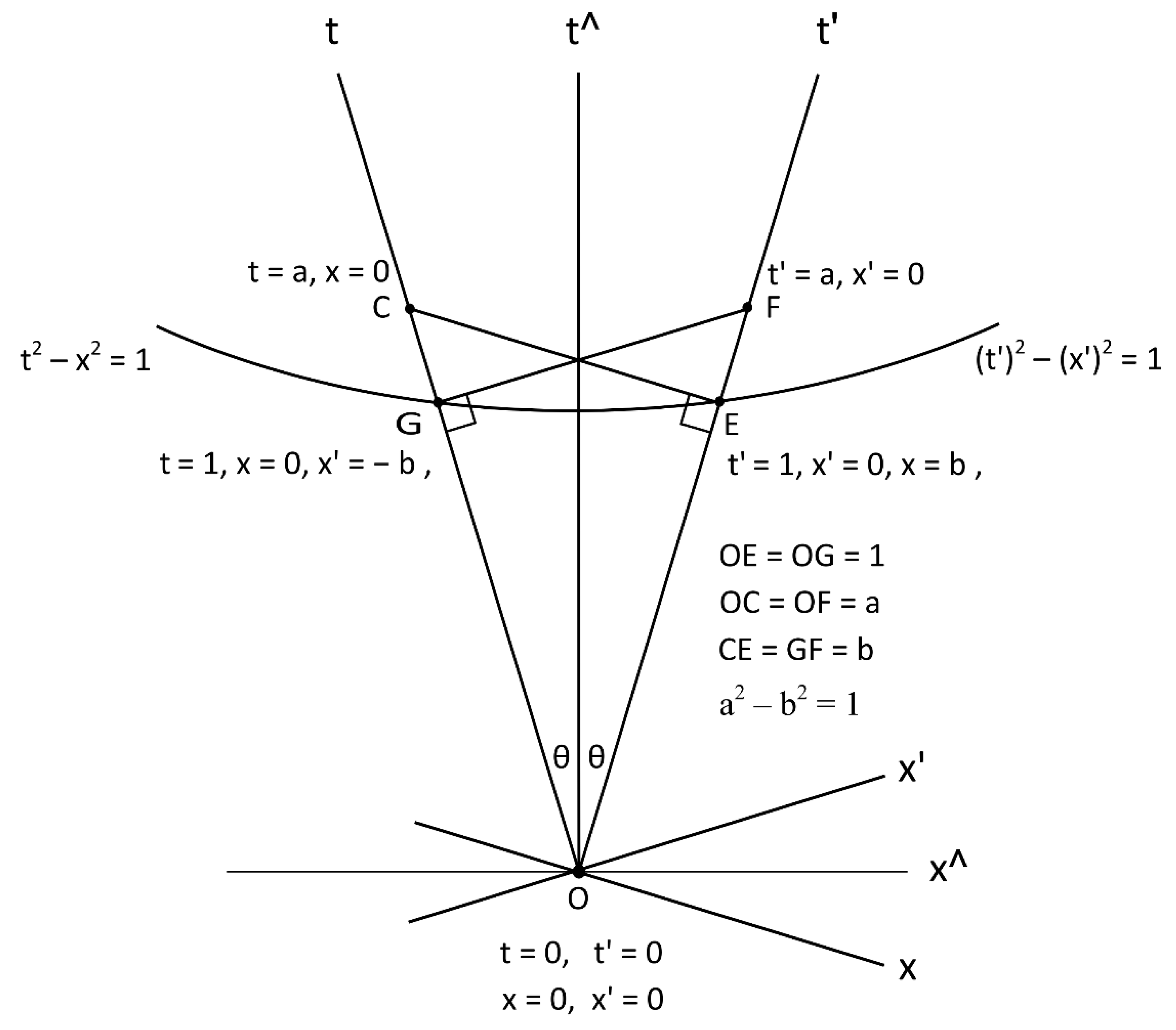
Central to the SRRM are the two congruent triangles OEC and OGF shown in Figure 1.

The lines OC and OF are, respectively, the time axis (worldline), t, of inertial observer Peter and the time axis (worldline), t′, of inertial observer Ruby. These lines diverge symmetrically from the origin, each at an angle θ either side of a vertical median t^ axis. The angle between the t and t′ axes is 2θ.

The lines CE and FG are, respectively, Peter’s x axis and Ruby’s x′ axis.

Results

The Equations and Terms in the SRRM

In triangles OEC and OGF there are the following relations.

a² = b² + 1

Cos 2θ = 1/a

Sin 2θ = b/a

Tan 2θ = b.

In the SRRM, the speed of light, c, is defined as 1. All velocity terms are expressed as a proportion of c. The transformation equations derived in the SRRM are:

x = ax′ + bt′

t = at′ + bx′

x′ = ax – bt

t′ = at – bx

Consistency of the Equations of the SRRM with Those of the Lorenz Transformation

The commonest form of the LT uses the terms:

v = \frac{x}{t}

c = the speed of light

γ = \frac{1}{\sqrt{1 - \frac{v^{2}}{c^{2}}}}

The LT equations are then:

x = γ (x′ +

v

t′)

t = γ (t′ +

v

x′∕c²)

x′ = γ (x –

v

t)

t′ = γ (t –

v

x∕c²)

A variation of the LT is that

v

/c is expressed as β. Thus,

v

= βc. The equations take the form:

x = γ (x′ + βct′)

ct = γ (ct′ + βx′)

γ = \frac{1}{\sqrt{1 - β^{2}}}

When c is defined as 1,

v

= β. The equations of the LT then take the form:

x = γ (x′ +

v

t′)

t = γ (t′ +

v

x′)

γ = \frac{1}{\sqrt{1 - v^{2}}}

Comparing the terms of the LT, when c is defined as 1, with those of the SRRM:

v = \frac{x}{t} = \frac{b}{a} = \frac{b}{\sqrt{1 + b^{2}}} = \frac{\sqrt{a^{2} - 1}}{a}

γ = \frac{1}{\sqrt{1 - \frac{b^{2}}{a^{2}}}} = \frac{1}{\sqrt{\frac{a^{2} - b^{2}}{a^{2}}}} = \frac{1}{\sqrt{\frac{1}{a^{2}}}} = a

b = a v = γ v = \frac{v}{\sqrt{1 - v^{2}}}

It is clear from the above that the terms and equations of the SRRM and those of the LT are completely interchangeable. The equations of the SRRM are simpler and the symmetry of the equations is more clearly shown. Hence, the underlying principles of special relativity can be more clearly seen.

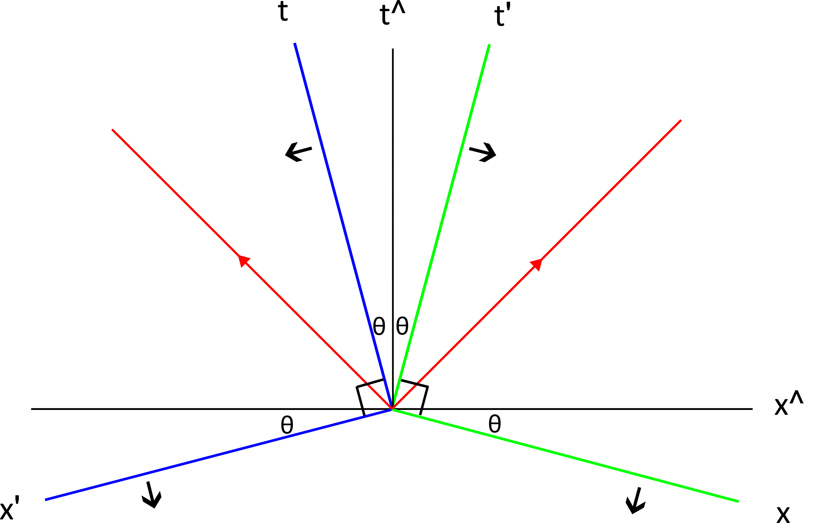
Mirror-Image Rotation of the Symmetrical Orthogonal Coordinate Systems

In the SRRM, as the angle [2θ] between the t and t′ axes increases, the t and t′ axes diverge symmetrically about the vertical t^ axis. The x′ and x axes maintain orthogonality, respectively, with the t and t′ axes at all values of θ (0 to +/– 45˚).

Figure 2. The anticlockwise rotation of the (x′, t) axes and the symmetrical clockwise rotation of the (x, t′) axes with increase of the angle [2θ] between the t and t′ axes in the SRRM .

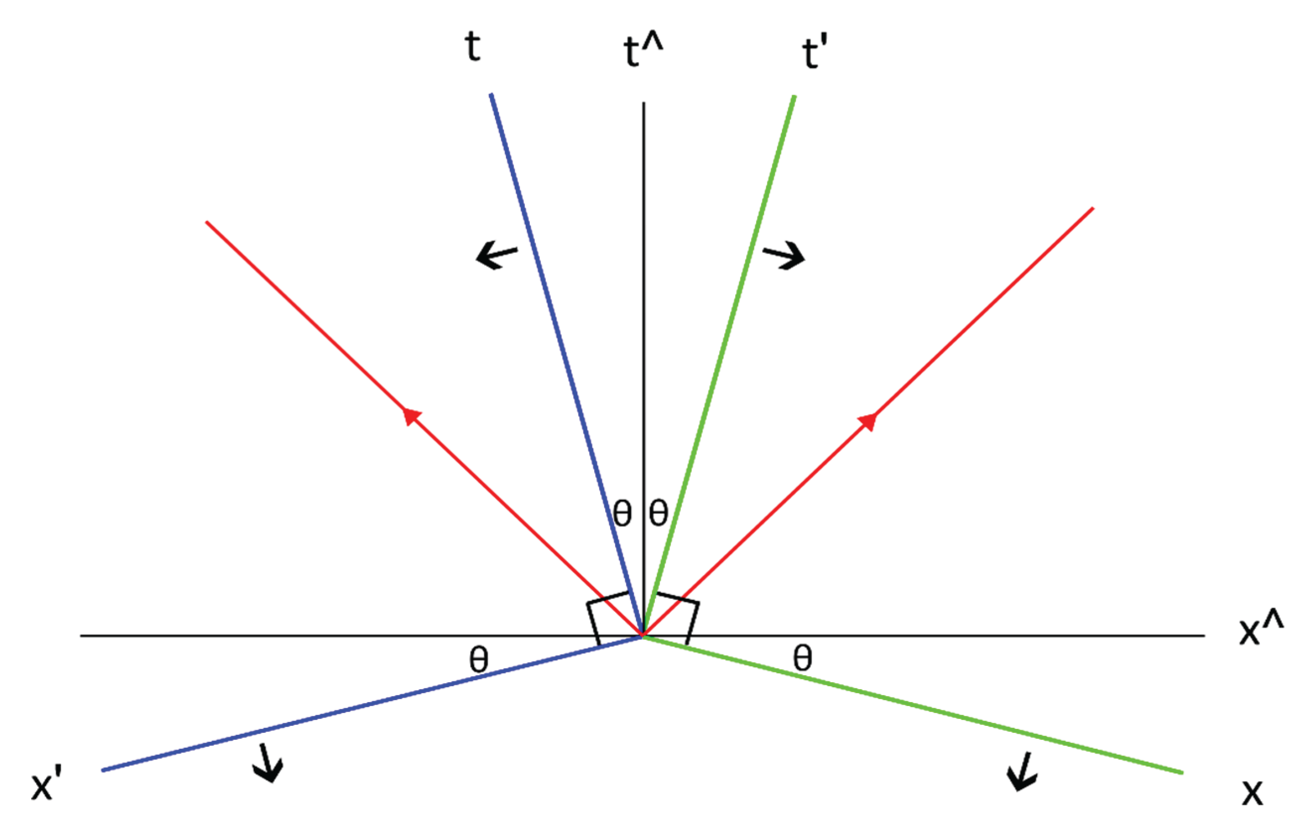
Thus, SOCS (x, t′) and (x′, t) have mirror-image rotation: the (x′, t) axes rotating anticlockwise; the (x, t′) axes rotating clockwise.

This geometrical finding in the SRRM is confirmed by the algebra of the transformation equations.

x = ax′ + bt′ x′ = x (1/a) – t′ (b/a) x′ = x Cos 2θ – t′ Sin 2θ

t′ = at – bx t = t′ (1/a) + x (b/a) t = x Sin 2θ + t′ Cos 2θ

This gives an anticlockwise rotation matrix for the orthogonal (x′, t) axes

[\begin{matrix} C o s 2 θ & - S i n 2 θ \\ S i n 2 θ & C o s 2 θ \end{matrix}]

x′ = ax – bt x = x′ (1/a) + t (b/a) x = x′ Cos 2θ + t Sin 2θ

t = at′ + bx′ t′ = – x′ (b/a) + t (1/a) t′ = – x′ Sin 2θ + t Cos 2θ

This gives a clockwise rotation matrix for the orthogonal (x, t′) axes

[\begin{matrix} C o s 2 θ & S i n 2 θ \\ - S i n 2 θ & C o s 2 θ \end{matrix}]

Discussion

Invariance of the Spacetime Interval Shown by Pythagoras

Several authors [3,4,5,6,10] have noted the two pairs of orthogonal axes in a Symmetrical Spacetime Diagram (SSD) and the fact that the typical equation for invariance of the spacetime interval

(∆t)² − (∆x)² = (∆t′)² − (∆x′)²

can be rewritten as (∆t)² + (∆x′)² = (∆t′)² + (∆x)²

where the invariance of the spacetime interval is shown by Pythagoras.

In 1962, Brehme [3] described his SSD.

“which needs neither the concept of imaginary numbers nor the use of scale changes….In order to use only Euclidian geometry, the equation

d s^{2} = d x^{2} - c^{2} d t^{2} = d {x'}^{2} - c^{2} d {t'}^{2}

is written with the terms rearranged:

d x^{2} + c^{2} d {t'}^{2} = d {x'}^{2} + c^{2} d t^{2}

The equation implies that if (x, ct′) are made the rectangular coordinates of one coordinate system and (x′, ct) the rectangular coordinates of another system rotated with respect to the first: the usual orthogonal transformation from one to the other will be the Lorenz transformation.”

In 1968, Sears and Brehme [4] referred to the interval L between two events in their SSD, the “Lorenz diagram”

“Because of the orthogonality of the (x_A, t_B) axes and the (x_B, t_A) axes, the lengths ∆x_A and c∆t_B form the arms of a right triangle with hypotenuse L, while ∆x_B and c∆t_A form another right triangle with the same hypotenuse. From the Pythagorean theorem, we know that

L^{2} {= c}^{2} ∆ t_{A}^{2} + ∆ x_{B}^{2} {= c}^{2} ∆ t_{B}^{2} + ∆ x_{A}^{2}

It follows that

{= c}^{2} ∆ t_{A}^{2} - ∆ x_{A}^{2} {= c}^{2} ∆ t_{B}^{2} - ∆ x_{B}^{2}

Since the A and B frames are arbitrary, the quantity c²∆t² – ∆x² is the same in all frames of reference, for a given pair of events, and is therefore an invariant quantity. The square of the invariant interval, ∆σ, is defined as ∆σ² = c²∆t² – ∆x² ”

Thus, Brehme, in his later work, simply used the Pythagorean invariance as a route to the squared invariant interval expressed as a difference of squares.

In 1968, Shadowitz [5] in showing how the Brehme diagram [3,4] is developed, wrote

“…we now have X² + c²t² = x² + c²T². X and cT are the coordinates, for one observer, of the event E; x and ct are the coordinates of the same event for another observer. Thus, here we have the important relation

X² – c²T² = x² – c²t ²

…this equation...is central to everything in special relativity.”

Thus, Shadowitz also saw the Pythagorean invariance just as a route to the invariant interval expressed as a difference of squares.

In 1996, Sartori [6] stated that:

“An ingenious alternative approach was discovered by Enrique Loedel. Loedel's construction is based on the realization that although (ct)² + x² is not invariant in relativity, the quantity (ct)² – x² is invariant. The relation

(ct)² – x² = (ct′)² – (x′)² (5.12)

which expresses that invariance, can be trivially rewritten as

(ct)² + (x′)² = (ct′)² + x² (5.13)

Equation (5.13) is formally analogous to the equation

x² + y² = (x′)² + (y′)²

which expresses the invariance of the distance …. This analogy led Loedel to construct the diagram ….in which the x axis is perpendicular not to the ct axis but to the ct' axis; the x' and ct axes are likewise perpendicular.”

Examining Loedel’s 1948 article [7] and the 1949 and 1955 books [8,9], while he refers to the orthogonal pairs of axes, no reference could be found to the equation

(ct)² + (x′)² = (ct′)² + x²

Thus, Sartori [6] saw the Pythagorean invariance (his 5.13) as the invariant interval expressed as a difference of squares (his 5.12) “trivially rewritten”

In 2012, Benedetto at al. [10] wrote:

“In our opinion …. the simplest way to introduce Loedel diagrams is through reducing Lorentz transformations, which relate two inertial reference frames, to a simple rotation of the axes through a real angle. The peculiarity of this rotation is the mix between the axes of the two systems: actually it is not a rotation of the (ct, x) frame with respect to the (ct′, x′) frame, but the rotation of (ct′, x) with respect to (ct, x′)”

Benedetto’s diagram showed the angle φ between the ct and ct′ axes. He continued:

“Lorenz transformations are…. ct′ = ct cos φ − x′ sin φ

x = ct sin φ + x′cos φ

The matrix

[\begin{matrix} C o s 2 φ & - S i n 2 φ \\ S i n 2 φ & C o s 2 φ \end{matrix}]

represents, as is well known, a standard clockwise rotation

of the real angle φ. So the Lorentz transformations have been expressed in terms of a rotation of the system (ct′, x) of an angle φ with respect to (ct, x′) frame.”

In summary, in 1962 Brehme [3] identified the invariance by Pythagoras as a rotation of one orthogonal coordinate system with respect to another. In 1968, Sears and Brehme [4] noted this, mainly as a route to expressing the invariant interval as a difference of squares. Shadowitz [5] and Sartori [6] had essentially the same approach. In 2012 Benedetto et al [10] described the clockwise rotational matrix related to the orthogonal (ct′, x) axes. However, they did not describe how the (ct, x′) axes symmetrically rotate anticlockwise resulting in the mirror-image rotation that has been described in the SRRM.

Interestingly, while the above authors have described the calculation of the invariant spacetime interval using Pythagoras with varying degrees of detail and interest, none of them have suggested that spacetime in special relativity could be fundamentally Euclidian.

Development of the SRRM

In developing the SRRM the main aim is to be consistent with the Principle of Relativity and display, graphically, the symmetry of the relative motion.

Gruner [11], in his symmetrical spacetime diagram, identified that there are pairs of orthogonal axes (x, t′) and (x′, t).

Brehme interpreted the two pairs of orthogonal axes in a symmetrical spacetime diagram as two coordinate systems and showed the invariance of the spacetime interval between those coordinate systems by Pythagoras.

The elegance of the algebra and geometry in what has now been called the SRRM leads to the conclusion that the SOCS (x, t′) and (x′, t) are fundamental in relative motion.

The SRRM is an accurate geometrical model of the algebra of special relativity. The geometry of the SRRM reveals the mirror image rotation of the SOCS that is consistent with the algebra.

The equation t² – x² = 1 is fully explained by the right-angle triangles OCE and OGF of the SRRM in Figure 1. No additional manipulation is needed to progress the mathematics.

Thus, in the SRRM, spacetime in special relativity is entirely explained by Euclidian geometry.

In view of this, in the transformation between the two SOCS (x, t′) and (x′, t), the fundamental equation of the invariant interval is (∆t)² + (∆x′)² = (∆t′)² + (∆x)².

The Definition of Velocity

The power of the simple and symmetrical transformation equations of the SRRM is shown as they describe the pair of SOCS that rotate as relative velocity increases.

It is surprising that Brehme, after identifying the pairs of orthogonal coordinate systems [3], appeared to lose interest in them [4]. It is more surprising that no-one subsequently except Benedetto et al. [10] have shown any interest in the SOCS. Perhaps, they have seen no fundamental significance in a combination of (x, t′) or (x′, t).

It has been shown in this article how important symmetry is in the understanding of special relativity. It would be an unequal balance if the fundamental measure of relative motion between two inertial bodies were to use both distance and time from the coordinate system of only one of the inertial observers.

The Galilean transformation is:

x′ = x – (velocity) x (universal time)

or x = x′ + (velocity) x (universal time)

The related transformation equations of the SRRM are:

x′ = ax – bt

x = ax′ + bt′

Thus, the velocity term, b, in the SRRM can simply replace the Galilean velocity term when a=1, as it is at low velocities where the Galilean transformation applies.

In view of the significance of the combination of (x, t′) or (x′, t) in the SOCS, the consideration of symmetry and the similarity to the Galilean transformation, there is good evidence to conclude that the velocity terms in the SRRM,

b = x/t′

or – b = x′/t

are the fundamental measures of velocity.

Conclusions

The conclusion is that spacetime in special relativity is Euclidean. There is good evidence that the fundamental definition of velocity is x/t′ or x′/t. The values x/t or x′/ t′ are a useful approximation.

Abbreviations

SRRM	Symmetrical Reflected Radar Model
SOCS	Symmetrical Orthogonal Coordinate Systems
LT	Lorenz Transformation
SSD	Symmetrical Spacetime Diagram

References

Asquith, P (2021) The Velocity Assumption. ISBN 9798772456378 Kindle Direct Publishing.
Asquith, P (2025) A Symmetrical Reflected Radar Model of Special Relativity using Euclidian Geometry. https://vixra.org/abs/2504.0064.
Brehme, R W (1962) A geometric representation of Galilean and Lorentz transformations Am. J. Phys. 30 489. [CrossRef]
Sears and Brehme (1968) Introduction to the Theory of Relativity. Addison-Wesley, NY.
Shadowitz, A (1968) Special Relativity (Philadelphia, PA: Saunders) https://archive.org/details/isbn_9780721681153.
Sartori, L (1996) Understanding Relativity: A Simplified Approach to Einstein’s Theories (LA, CA: UCP) https://archive.org/details/understandingrel0000sart.
Loedel, E (1948) Aberración y Relatividad (Aberration and Relativity) Anales de la Sociedad Cientifica Argentina. 145: 3-13. https://archive.org/details/Loedel1948AberracionYRelatividad/mode/2up.
Loedel, E (1949) Enseñanza de la Física. Editorial Kapelusz. Buenos Aires https://archive.org/details/LoedelEnsenanza/page/n527/mode/2up.
Loedel, E. (1955) Fisica Relativista https://archive.org/details/LoedelFisicaRelativista1955.
Benedetto et al. (2013) Some remarks about underused Loedel diagrams. Eur. J. Phys. 34 67-74. [CrossRef]
Gruner, P (1922). Elemente der Relativitätstheorie [Elements of the theory of relativity] (in German). Bern: P. Haupt.
Minkowski, H (1908) “Space and Time”. Address delivered at the 80th Assembly of German Natural Scientists and Physicians, Cologne. In “The Principle of Relativity,” Dover Publications, New York, 1923 https://archive.org/details/principleofrelat00lore_0/page/74/mode/2up.

Figure 1. The key congruent triangles, OEC and OGF, of the Symmetrical Reflected Radar Model.

Disclaimer/Publisher’s Note: The statements, opinions and data contained in all publications are solely those of the individual author(s) and contributor(s) and not of MDPI and/or the editor(s). MDPI and/or the editor(s) disclaim responsibility for any injury to people or property resulting from any ideas, methods, instructions or products referred to in the content.

© 2025 by the authors. Licensee MDPI, Basel, Switzerland. This article is an open access article distributed under the terms and conditions of the Creative Commons Attribution (CC BY) license (http://creativecommons.org/licenses/by/4.0/).

Copyright: This open access article is published under a Creative Commons CC BY 4.0 license, which permit the free download, distribution, and reuse, provided that the author and preprint are cited in any reuse.