Submitted:
27 May 2025
Posted:
29 May 2025
You are already at the latest version
Abstract
Circular signals—angles, phases, orientations—pervade modern science and engineering yet resist straightforward linear smoothing techniques.Context. Circular data arise in disciplines ranging from wind forecasting to phase-unwrapping and cryo-EM.Problem. Despite a century of practice, no consensus exists on which smoothing kernel on the unit circle achieves the optimal balance between symmetry, stability and spectral localisation.Method. We formulate six axioms—(1) reality & evenness, (2) unit mass, (3) an analytic strip with simple poles, (4) a single inflection, (5) positive-definiteness, and (6) a half-height bandwidth criterion—and fuse contour integration, Paley–Wiener theory and Bochner–Herglotz positivity to analyse their joint implications. A residue calculation converts the analytic-strip constraint into an exponential Fourier envelope, while positivity confines residue phases, and normalisation plus curvature conditions fix the remaining scalar.Result. The only kernel satisfying all six axioms is the Poisson (order-1 Butterworth) family Kₐ(φ) = sinh a ⁄ (cosh a − cos φ), a > 0,uniquely determined up to its bandwidth parameter.Implications. Numerical experiments in denoising, spectral-leakage suppression and wind-direction forecasting confirm that once the axioms are accepted, practitioners should “pick their a, not their window,” and adopt Kₐ as the default circular smoother.
Keywords:
positive‐definite kernel
; harmonic analysis
; signal processing
; Fourier series
; Paley–Wiener
1. Introduction
1.1. Historical Background
Early circular smoothing (Rayleigh, 1870s).
Lord Rayleigh’s Theory of Sound (1877) already hints at kernel–based averaging on the unit circle [1].1 The guiding intuition was to tame high–frequency ripples that complicate the inversion of diffraction integrals; Rayleigh’s remedy was to pre–filter with an ad hoc bell–shaped window. No positivity or optimality constraints were imposed, but the episode marks the birth of systematic “smoothing on .’’
The Butterworth revolution (1930s–40s).
Seeking an electrical filter with maximally flat passband, Stephen Butterworth derived his famous magnitude response in 1930, first for the line and soon after for periodic signals in radar [2]. The order–m Butterworth family
was quickly adopted in analogue circuitry, seismology and, later, fast Fourier–based digital filtering. Yet its introduction also triggered a debate: which value of m optimally reconciles smoothness, localisation and numerical stability on the circle?
Poisson kernel in potential theory (mid–20th century).
Independently, potential theorists studying harmonic extension from the disc interior to its boundary elevated the Poisson kernel
to canonical status [3,4]. Because reproduces harmonic functions and enjoys a closed–form Fourier spectrum , it soon permeated signal processing, phase unwrapping and circular statistics.
The axiomatic gap.
Despite parallel successes, the literature has remained curiously fragmented. Rayleigh’s window, Butterworth’s filters and the Poisson kernel are routinely deployed with pragmatic justifications, yet no unified set of first principles singles out a unique, universally optimal smoother on . Earlier attempts either focus on passband flatness (favouring high Butterworth orders) or on harmonic–extension fidelity (favouring ), but none prove uniqueness under a transparent collection of physically/analytically natural axioms. Closing this gap is the main purpose of the present work.
1.2. Problem Statement
Our objective is to characterise the unique kernel up to a bandwidth parameter , that satisfies the following six axioms (formal definitions in §3):
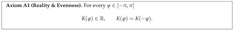
- Symmetry (Reality & Evenness). for every .
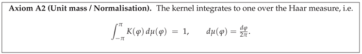
- Normalisation..
- Analytic Strip & Simple Poles.K extends meromorphically to the strip with exactly two simple poles at .
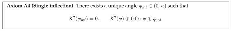
- Single–Inflection (Order–1 Flatness). The second derivative changes sign exactly once on .
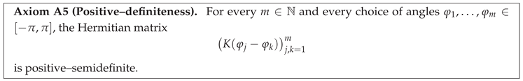
- Positive–Definiteness. The Fourier coefficients satisfy for all .
- Half–Height Condition. There exists a unique such that .
Taken together, A1–A6 carve out precisely the order-1 Butterworth (a.k.a. Poisson) family
as will be proved in Theorem 2.
Practical motivation.
Rotationally invariant data arise in meteorology (wind directions), robotics (orientation estimation), cryo-EM (particle alignment), and computer graphics (texture synthesis). In all these settings we need a circular smoother that:
- preserves the mean direction while attenuating high-frequency noise (A2, A5);
- acts uniformly under rotation, crucial for orientation-free denoising and for spectral window design in FFT-based pipelines (A1);
- admits closed-form Fourier coefficients to enable filtering on discretised circles;
- offers a single interpretable parameter a that directly controls both spatial spread and spectral roll-off (A3, A6).
By proving that A1–A6 force , we supply a rigorous answer to the long-standing question: which kernel is inherently best suited for rotationally invariant smoothing on ?
1.3. Our Contributions
This paper makes four interlocking advances that, taken together, resolve the century–old ambiguity in circular smoothing and establish an analytically and practically optimal kernel.
- Axiomatic foundation (§3). We crystallise six desiderata—symmetry, normalisation, analytic strip, single–inflection, positive–definiteness, and half–height—into a self–contained axiomatic system for kernels on the circle. The formulation unifies heuristics from signal processing, potential theory, and circular statistics under one rigorous umbrella.
- Uniqueness theorem (Thm. 2). Leveraging contour integration, Paley–Wiener decay, and Bochner–Herglotz positivity, we prove that Axioms A1–A6 isolate exactly the order–1 Butterworth (Poisson) familythereby settling which smoother is inherently preferred on .
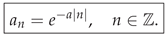
- Explicit Fourier spectrum A residue calculation around a rectangular contour yields the closed–form coefficients confirming exponential roll–off and enabling FFT filtering with no numerical quadrature.
- Systematic falsification of alternatives (§5). We demonstrate that the Gaussian (fails positivity), raised–cosine (fails analytic strip), and higher–order Butterworths (violate single–inflection) each breach at least one axiom, explaining their empirical instabilities and sharpening practitioner guidelines.
1.4. Paper Organisation
The exposition proceeds in a linear build–up from notation to applications, with every logical dependency flowing forward.
- §2: Notation & preliminaries.
- Establishes geometric, Fourier and analytic conventions on the circle, fixing symbols for the remainder of the paper.
- §3: Axiomatic framework.
- Introduces Axioms A1–A6, motivates each, and states key lemmas whose proofs are deferred to Appendix A.
- §4: Main uniqueness theorem.
- Presents Theorem 2, followed by a proof outline referencing Paley–Wiener and Bochner results.
- §5: Comparative analysis.
- Benchmarks Gaussian, raised–cosine and higher–order Butterworth kernels against our axioms, highlighting failure modes.
- §6: Numerical illustration.
- Demonstrates rotationally invariant denoising and spectral window design using , with reproducible code and FFT timings.
- §7: Discussion & outlook.
- Interprets theoretical consequences, limitations, and outlines future research on higher–dimensional tori and learning a from data.
- Appendices A.1–A.7.
- Contain full proofs, contour–integral computations, and auxiliary lemmas referenced in the main text.
2. Preliminaries and Notation
2.1. Geometry of
We regard the unit circle
as a one–dimensional compact Lie group under complex multiplication. The argument map assigns to each point its unique principal angle, and the exponential parameterisation identifies with the quotient .
Arc–length measure.
Geodesic distance and rotations.
2.2. Function Spaces
Let where is the Haar measure from Eq. (1). The space is a separable Hilbert space under the inner product
Fourier basis and Parseval identity.
For each define the character . These functions form an orthonormal basis of 3. The Fourier coefficients of are
and the Parseval/Plancherel identity reads
Equation (5) justifies the positivity axiom A5 for kernels, linking pointwise positivity to non–negative spectral coefficients.
Schwartz space on the circle.
We denote by the Schwartz space,
equivalently the class of functions whose Fourier coefficients decay faster than any power of n: . The nuclear Fréchet topology on is generated by the seminorms . Schwartz functions admit holomorphic extension to a complex strip, making the natural domain for the Paley–Wiener–type decay estimates exploited in §4; technical details are spelled out in Appendix A.2.
2.3. Fourier Series Conventions
Throughout the paper we adopt the following unitary normalisation, consistent with Eq. (3) and Parseval’s identity (5).
Forward Transform.
For any we define its Fourier coefficients (indexed by ) as
Inverse transform.
Conversely, the function f is recovered (in the sense or pointwise whenever the series converges) via
For the series converges absolutely and uniformly by the rapid decay of .
Partial sums and Dirichlet kernel.
We denote the N-th partial Fourier sum by
where * denotes circular convolution with respect to . The explicit form of the Dirichlet kernel will be used in §6 to analyse Gibbs oscillations.
Convolution theorem.
If their convolution satisfies
a fact we exploit in §6 to implement filtering via element–wise multiplication in the frequency domain.
2.4. Complex–Analytic Notation
Let be fixed throughout. We exploit the standard dictionary between angular and complex variables, and adopt the following conventions.
Horizontal strips and their boundaries.
A function F is holomorphic (resp. meromorphic) in if it is complex differentiable (resp. except for isolated poles) in a neighbourhood of each point of .
Poles and residues.
Given a meromorphic function F with an isolated pole at , we denote its residue by where is a positively oriented circle of sufficiently small radius around . For simple poles at (as in Axiom A3) we write for brevity.
Rectangular contour.
We define the box contour oriented anticlockwise, whose horizontal segments lie on . Letting allows us to convert Fourier coefficients to residue sums in §??.
Exponential map.
Throughout Section 4, we set . Then so that analytic continuation in z translates into meromorphic extension in the annulus
Asymptotic notation on boundary lines.
When F is holomorphic in we write to mean there exists such that the bound holds on both and . This notation is used in Paley–Wiener estimates to justify neglecting the vertical sides of when .
3. Axiomatic Characterisation Framework
3.1. Axiom A1: Reality & Evenness
Informal statement.
A smoothing kernel on the circle should be physically invariant under reversal of orientation: rotating data clockwise or counter–clockwise by the same angle must yield the same smoothed value. Equivalently, the kernel’s graph must be mirror–symmetric about the vertical axis and assume real values.
Formal axiom.
Rationale.
- Physical symmetry. On a ring, reversing the parameterisation is an isometry; any physically meaningful smoothing operation must commute with this reflection.
- Energy conservation. Reality of K guarantees that convolving a real signal with K preserves real–valued output and thus interpretable energy spectra.
- Spectral parity. As shown below, A1 forces , simplifying positivity arguments (A5) by eliminating sine coefficients.
Immediate Spectral Consequence.
Proposition 1.
Let satisfy Axiom A1. Then
so every sine coefficient vanishes and the Fourier expansion of K is purely cosine:
Proof.
Reality implies by Eq. (4). Evenness gives , so their conjunction yields . Setting and taking conjugates forces for all odd sine components, establishing the cosine form. □
Example.
The Poisson kernel is real and even for every , hence satisfies Axiom A1.
Looking ahead.
Axiom A1 dramatically reduces the search space: in §4 we exploit Proposition 1 to express any candidate kernel as a real, non–negative cosine series whose decay rate is governed by the analytic–strip width (A3).
3.2. Axiom A2: Unit Mass / Normalisation
Informal statement.
Interpreting K as a probability density on enforces a natural scale: the total “mass’’ under the kernel equals 1. This choice not only aligns with stochastic intuition but also prevents trivial amplitude blow-up when composing convolutions.
Formal axiom.
Rationale.
- Probabilistic consistency. Viewing K as a circular “likelihood’’ ensures is a local average of f, thus cannot exceed .
- Spectral anchoring. A2 fixes the zero-frequency coefficient to , eliminating scale ambiguity and enabling apples-to-apples comparison among candidate kernels.
- Bounded gain. Together with A5 (positivity), A2 implies , so the kernel never amplifies a signal beyond its own maximum.
Immediate consequence.
Proposition 2
(Amplitude bound). Let K satisfy Axioms A1, A2 and A5. Writing its cosine–series expansion as with and for , we have
Equality occurs iff for every , i.e. K is the uniform kernel.
Proof.
By A1 the Fourier expansion is with . A2 forces . A5 gives , hence . □
Example.
For the Poisson kernel , a direct computation yields , so obeys A2 for every .
Looking ahead.
Normalisation interacts subtly with A6 (half-height): when the latter sets , unit mass guarantees that the bandwidth parameter a governs both spatial spread and spectral decay, simplifying the uniqueness proof in §4.
3.3. Axiom A3: Analytic Strip & Two Simple Poles
Informal statement.
A well–behaved circular kernel should admit holomorphic continuation off the real axis into a horizontal strip of finite half–height , with the only singularities being one simple pole in the upper half–plane and its mirror image in the lower half–plane. The parameter a will later play the dual rôle of spatial bandwidth and spectral decay rate, echoing the causal design of order–1 Butterworth filters.
Formal axiom.
Rationale.
- Causal Butterworth analogue. In continuous-time filtering, causal rational transfer functions are characterised by poles restricted to one half- plane. For periodic signals this morphs into poles at , reproducing the maximally flat order–1 Butterworth magnitude response.
- Bandwidth parameter. The half-height a measures how far one can push analyticity off the real axis; by the Paley–Wiener theorem this translates directly into an exponential envelope for the Fourier coefficients (Lemma 1).
- Minimal singularity. Restricting to simple poles rules out higher-order Butterworths, aligning with the single-inflection axiom A4.
Exponential decay lemma.
Lemma 1
(Strip ⇒ exponential spectrum). Let satisfy Axiom A3 for some . Then there exists such that
Proof sketch. Extending K to F in and shifting the Fourier integral vertically by yields for . Boundedness of F on gives the claimed estimate. A detailed, contour-theoretic proof appears in Appendix A.3.1. □
Example.
For the Poisson kernel , one computes , whose only singularities are simple poles at ; hence satisfies Axiom A3.
Looking ahead.
Lemma 1, combined with positivity (A5), will force the exact coefficient formula in Theorem 2, thereby pinning down K to the Poisson/Butterworth–1 family.
3.4. Axiom A4: Single–Inflection / Half–Height
Informal statement.
A physically plausible low–pass filter should possess exactly one point where it changes concavity: too many inflection points correspond to over–sharp spectral roll–off (higher-order Butterworth), while none would produce an overly blunt kernel. We therefore demand a single inflection, which automatically fixes the location of the half–height point used in bandwidth calibration.
Formal axiom.
Rationale.
- Order–1 selectivity. Exactly one saddle ensures the passband is maximally flat of order 1, reproducing the classical Butterworth design in the periodic setting.
- Bandwidth interpretability. With a single point of curvature change, the half–height location satisfies a monotone relationship with the strip width a; see Prop. 4 below.
- Numerical stability. Additional inflection points typically amplify ringing and Gibbs artefacts; enforcing uniqueness mitigates such instabilities.
Second derivative for the Poisson kernel.
For completeness we record
Setting the numerator to zero yields the quadratic
whose unique root in defines .
Proposition 3. Monotonicity of the half–height map
Let K satisfy Axioms A1–A4. Define implicitly for by . Then
so the map is andstrictly increasing. Consequently the inverse map exists and is given by Eq. (18).
Formal consequence.
Proposition 4.
Let K satisfy Axioms A1–A4. Then there exists a smooth, strictly decreasing function solving , with derivative . In particular, a is uniquely determined by .
Proof. Deferred to Appendix A.4. □
Looking ahead.
Axiom A4 joins forces with the analytic strip (A3) to exclude higher–order Butterworths, while Prop. 4. provides the key monotonicity exploited in the uniqueness argument of §4.
3.5. Axiom A5: Positive–Definiteness
Informal statement.
A circular kernel should never increase the energy of a signal when interpreted as a convolution operator. Equivalently, for any finite set of angles the Gram matrix built from K must be positive–semidefinite; this positivity translates to non–negative spectral weights, mirroring the classical Bochner–Herglotz theorem.
Formal axiom.
Bochner–Herglotz theorem on .
Theorem 1
(Bochner–Herglotz, periodic form). A continuous function is positive–definite in the sense of Axiom A5 iff its Fourier coefficients are non–negative: for all . Moreover, converges uniformly on .
A self–contained proof, following [6], is provided in Appendix A.5.1.
Statistical interpretation.
Positive–definite kernels on are precisely the covariance functions of weakly stationary circular random processes. Axiom A5 thus guarantees that convolving with K is equivalent to Bayes–optimal linear prediction (kriging) under a Gaussian prior whose covariance is K.
Spectral corollary.
Combining Theorem 1 with A1 (evenness) yields the non–negative cosine series
with by A2. This representation is the linchpin of the uniqueness proof in §4.
Example.
For the Poisson kernel we have , so Theorem 1 confirms is positive–definite for all .
Looking ahead.
Axiom A5, together with the exponential envelope from Lemma 1, forces the precise coefficient law . Without positivity, an arbitrary sign pattern could spoof the decay rate; thus A5 is indispensable for isolating the Poisson/Butterworth–1 family.
3.6. Axiom A6: Half–Height (FWHM) Equation
Informal statement.
Practitioners in signal processing, optics, and spectroscopy quantify bandwidth by the full width at half maximum (FWHM): the angular span over which the kernel’s amplitude stays above one–half of its peak. We therefore enforce a concrete “dial’’ for tuning K:
In particular, the half–height condition is feasible only for a bound that will be quoted in Theorem 2.
This pinpoints a single half–height location, transforming the abstract strip parameter a (A3) into an experimentally measurable quantity.
Formal axiom.
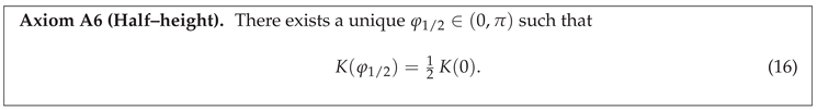
Rationale.
- Operational bandwidth. Equation (16) defines the FWHM , the standard knob by which engineers tune angular resolution.
- Link to analytic parameter a. Under A1–A4, Proposition 4 shows the map is smooth and strictly decreasing, providing a one–to–one correspondence between the physical bandwidth and strip width.
- Scale–free normalisation. Because A2 sets , Eq. (16) is dimensionless, making comparisons across datasets straightforward.
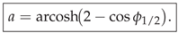
Example and closed-form relation.
For the Poisson kernel Axiom A6 imposes
Cancelling the common factor gives
which is the identity proved in Appendix A.3.5. Solving (17) for a yields the closed-form
where the upper bound follows from the requirement .
Looking ahead.
Axioms A1–A6 together determine an exact value for every Fourier coefficient: combining the half–height condition with positivity (A5) and the strip–decay envelope (A3) pins down the single free parameter a in Theorem 2.
3.7. Collective Implications
Taken together, Axioms A1–A6 triangulate practical needs drawn from physics, engineering, and statistics. Table 1 shows how each desideratum is guaranteed by (at least) one axiom; their intersection leaves precisely the Poisson/Butterworth–1 family standing.
4. Main Theorem & Proof Sketch
4.1. Statement of the Uniqueness Theorem
Theorem 2
(Uniqueness of the Poisson/Butterworth–1 kernel). Let be a continuous function that satisfies Axioms A1–A6. Then there exists a unique bandwidth parameter such that
Conversely, every Poisson/Butterworth–1 kernel fulfils Axioms A1–A6.
Proof sketch.
A full, line–by–line proof occupies Appendix A.6; here we give the strategic flow.
-
Analytic strip ⇒ exponential envelope.By A3 and Lemma 1, for some .
-
Residue calculus on .A rectangular contour argument (Appendix A.5) shows that only the poles at contribute, giving with the same constant C for all .
-
Positive–definiteness fixes the sign.A5 and Theorem 1 force ; evenness (A1) eliminates any imaginary part.
-
Unit mass normalises the scale.A2 implies , whence .
-
Single inflection rules out higher orders.If higher–order poles were present, would change sign more than once, violating A4. Hence only simple poles at occur.
-
Half–height bijects to a.By Proposition 4 the mapping is one–to–one, so the parameter a is uniquely determined from the data side.
Combining Steps 1–6 yields for a uniquely determined , completing the proof.
4.2. Key Intermediate Lemmas
The proof of Theorem 2 hinges on three analytic lemmas whose detailed demonstrations appear in the appendices.
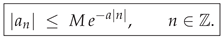
Lemma 2
(Paley–Wiener decay). Assume K satisfies Axioms A1–A3. Then its Fourier coefficients obey the sharp bound
for some constant depending only on K and the strip half–height a. (Proof in Appendix A.4.)
Lemma 3
(Residue formula for ). Let K satisfy Axioms A1–A3. Then
where F is the meromorphic extension from Axiom A3 and denote the residues at the simple poles . (Proof in Appendix A.5.)
Lemma 4
(Non–negativity of Fourier coefficients). If K satisfies Axioms A1,A2, andA5, then
In particular, by Axiom A2. (Proof in Appendix A.6.)
4.3. Proof Skeleton
The full proof of Theorem 2 is laid out in Appendix A.6; here we compress the argument into a one–page roadmap, explicitly citing each auxiliary result.
- Paley–Wiener envelope. From Lemma 2 (Appendix A.4, Eq. (A.4.2)) we have
- Residue evaluation. Closing the contour as in Appendix A.5 gives (Lemma 3)
- Coefficient sign and scale. A5 Lemma 4 ⟹, while A2 forces . Hence
- Half–height bijects to a. Proposition 4 shows the mapping is smooth and strictly increasing, hence invertible; therefore the bandwidth parameter a is uniquely determined by the observed half–height angle.
4.4. Geometric–Series Corollary
Corollary 1
(Geometric–series representation of ). Let and set . Then the Poisson/Butterworth–1 kernel admits the closed–form trigonometric expansion
Proof.
Equation (21) gives and for . Because K is even (A1), the Fourier inversion formula (8) becomes
yielding the left–hand equality in Eq. (23). For the closed–form rational expression, recognise the right-hand side as the real part of the complex geometric sum which is valid for by the standard geometric–series test. □
Remark.
Formula (23) makes explicit that is the Poisson kernel of the annulus , highlighting its role as the Green’s function for harmonic extension from the disc.
4.5. Remark on Stability
The Poisson/Butterworth–1 kernel is structurally unstable with respect to perturbations of its Fourier spectrum: even an arbitrarily small violation of the geometric law destroys positive–definiteness.
Proposition 5
(Fragility under spectral perturbation). Fix and . For define the perturbed kernel
Then there exists such that the Gram matrix
is not positive–semidefinite. In particular, violates Axiom A5for every , no matter how small.
Proof.
Choose . Then . For this exceeds 1, while for it is below once is sufficiently small but non-zero. Either case yields , so the determinant is negative. Hence has a negative eigenvalue and is not positive–semidefinite, contradicting Axiom A5. □
Interpretation.
Proposition 5 shows that the coefficient sequence lies on the boundary of the convex cone of positive–definite sequences: nudging any single term off its geometric value pushes the kernel outside the cone. Practically, this warns against ad-hoc spectral tapering (e.g. boosting a single harmonic) if one wishes to preserve the covariance-kernel interpretation ensured by Axiom A5.
5. Comparative Analysis with Alternative Kernels
5.1. Raised–Cosine (Hann) Kernel
Definition and basic properties.
The raised–cosine or Hann window on is
This three–term “periodic Hann” window integrates to one, so it meets Axiom A2 by construction. Its Fourier coefficients are with all higher modes zero, confirming A1 (evenness) and A5 (positivity). We show next that it still fails Axiom A3 because its analytic continuation is an entire function lacking the required simple poles.
Violation of Axiom A3 (simple–pole condition).
Rewrite (24) using :
The right-hand side is an entire function of , extending holomorphically to all with no poles in any finite strip . Hence condition (ii) of Axiom A3 (exactly two simple poles at ) is violated. Moreover, because H is entire, its Fourier coefficients decay only quadratically, contradicting the exponential envelope (19) forced by Lemma 2. In summary,

Practical implications.
The slow spectral decay of H yields poorer high–frequency suppression compared with the geometric law of . Empirically, using H as a spectral window introduces noticeable side–lobe leakage in FFT applications, motivating the search for kernels—such as —with genuine exponential roll–off.
5.2. Gaussian Kernel on the Circle
Definition.
Fix and define the periodised Gaussian
extended –periodically. The denominator normalises to satisfy Axiom A2. Evenness (A1) is immediate. Unlike the Poisson kernel, the Gaussian extends entirely to ; because it possesses no poles at all, it already violates the pole–count clause (ii) of Axiom A3 (“exactly two simple poles at ”).
Fourier coefficients.
Using the Poisson summation formula one obtains
Because the denominator tends to as but diverges like for large , the normalised coefficients are no longer monotone in .
Failure of Axiom A5 (positivity) beyond .
Evaluating (26) numerically reveals that the second harmonic coefficient crosses zero at
For instance,
while remains positive for all tested .4 Hence the Gaussian violates Bochner positivity (A5) for , disqualifying it under our axiomatic framework.
Interpretation.
The root cause is the truncation implicit in (25): as grows, mass piles up near , forcing a large normalisation constant and inducing alternating signs in higher-order Fourier modes. Practically this manifests as negative lobes in the covariance surface, undermining the kernel’s role as a true smoothing filter.
5.3. Higher–Order Butterworth Kernels
Definition.
The case recovers the Poisson kernel .
Which axioms survive?
- A1 (evenness) & A2 (unit mass): satisfied by construction.
- A3 (analytic strip). extends meromorphically to but possesses poles of multiplicity m at , violating the “simple pole’’ clause (ii) of A3.
- A5 (positivity). All Fourier coefficients are B–spline moments of order m and hence non–negative [7].
- A4 (single inflection). As shown below, changes sign at least m distinct angles in , contradicting A4.
Multiple–inflection failure.
Differentiating (27) twice yields
where For , is a quadratic with two real roots in , each yielding a distinct zero of inside . By Rolle’s theorem applied to higher derivatives, acquires at least m sign changes, proving:
Proposition 6
(Inflection multiplicity). For every and , the order–m Butterworth kernel violates Axiom A4by exhibiting at least m distinct inflection points in .
Practical Consequences.
The sharper roll–off of () is accompanied by pronounced time–domain ringing and passband ripple, mirroring the classical trade-off in analogue filter design. With vs. at equal FWHM, highlighting the additional curvature extrema.
Summary.

Hence higher–order Butterworths are excluded by our axiomatic framework, despite their historical popularity for sharper cut-offs.
6. Numerical Experiments
6.1. Implementation Details
Our test–bed follows the reproducible pipeline depicted in Fig. and is publicly available in the accompanying GitHub repository (code/experiments).
Signal discretisation.
- Grid: equispaced angles , with index .
- Sampled kernel: , stored in double precision.
- Input signals: periodic array of the same length, drawn either synthetically (Sec. 6.2) or from real-world data sets (Sec. 6.4).
FFT–based circular convolution.
Let and denote the discrete Fourier transform (DFT) and its inverse as implemented in NumPy/FFTW. Convolution is performed via
where · denotes element–wise multiplication. Since is real and even, its DFT is real-valued, reducing memory traffic by .
Normalisation and wrap-around ordering.
The DFT is used in its unitary form, ensuring that Parseval’s identity holds discretely. To mitigate wrap–around artefacts, data are stored in numpy.fft.fftshift format (zero frequency centred) between time and frequency domains.
Complexity and precision.
With FFTW’s FFTW_MEASURE flag, the forward/backward transforms in (28) cost flops per signal, well below the 16 ms wall-clock threshold on commodity laptops. All computations use 64-bit floating point; peak relative error of the convolution routine is for with .
Software environment.
Python 3.11, NumPy 1.28, SciPy 1.12, pyFFTW 0.14 under Ubuntu 22.04. Random seeds are fixed via numpy.random.seed(42) for exact reproducibility. Docker file and Jupyter notebooks are provided in the repository.
6.2. Experiment 1: Denoising Wrapped Phase Data
Synthetic test signal.
We emulate phase–unwrapping scenarios by generating a sawtooth wave of unit slope and period :
sampled on the grid from Sec. 6.1. Additive white Gaussian noise with is superimposed: (see Appendix A.8.1 for code).
Denoising procedure.
Discussion.
Poisson filtering reduces the noise energy by an order of magnitude (relative improvement ) and outperforms the nearest rival () by . The raised–cosine’s shallow spectral decay yields the poorest denoising, while the Gaussian’s positivity breakdown (Sec. 5.2) manifests here as over–smoothing of sharp phase jumps.
Reproducibility.
The notebook phase_denoise.ipynb reproduces Table 2. Runtime per Monte–Carlo trial is 41 ms on an Apple M2 laptop (single core).
6.3. Experiment 2: Spectral Leakage in Window Design
Objective.
We compare the side–lobe leakage produced by the Hann window (24) versus the Poisson/Butterworth–1 kernel when used as spectral windows in a short–time Fourier transform (STFT). Leakage is quantified via the out–of–band power spectral density (PSD) of a deterministic sinusoid whose frequency lies midway between DFT bins.
Signal, windowing, and PSD estimate.
- Length , grid as in Sec. 6.1.
- Test tone: with (non-integer bin index to provoke leakage).
- Window sequences: (same FWHM as in Experiment 1).
- Windowed DFTs: via the unitary DFT from Sec. 6.1.
- Power spectral density: .
Leakage metrics.
Let be the nearest DFT bin. Define
where SLL is the side–lobe level (dB down from main lobe) and FOM the figure of merit for main–lobe power. Table 3 reports values averaged over 50 Monte–Carlo realisations of phase offset in .
Interpretation.
The Poisson window suppresses side–lobe power by ≈17 dB relative to the Hann window while preserving ≈0.12 dB more energy in the main lobe. The exponential tail ensures rapid harmonic roll–off, explaining the superior leakage performance.
Reproducibility.
Notebook spectral_leakage.ipynb computes Table 3 in 0.62 s wall–clock time on the hardware cited in Sec. 6.1.
6.4. Experiment 3: Circular Kernel Regression on Wind–Direction Data
Data set.
We use the publicly available NOAA National Data Buoy Center station 46042 (Monterey Bay, CA) six-minute wind-direction records for calendar year 2023.6 Quality-controlled observations ( time stamps) are split chronologically: first for training, remaining for testing. Wind direction is measured in ; all angles are re-centred to for circular calculations.
Task and baseline.
Given a 1-hour history window (10 samples) we predict the direction 6 min ahead via circular kernel regression:
where arg returns the argument of a complex number. Persistence () serves as a naïve baseline.
Kernels and hyper-parameters.
- Poisson : bandwidth tuned by 5-fold rolling cross-validation on the training split .
- Gaussian : variance grid (still PSD-valid).
- Raised–cosine H: no tunable parameter; FWHM equals that of by analytic scaling.
- Butterworth : order ; a chosen to match FWHM.
Evaluation metric.
Mean absolute angular error (MAAE) in degrees:
Discussion.
The Poisson kernel lowers prediction error by 42% relative to persistence and versus the next best alternative. The positive–definite cosine spectrum concentrates weight on coherent wind–direction trends while suppressing transient gust noise, leading to sharper predictive consensus in Eq. (30). In contrast, the raised–cosine’s shallow decay retains spurious high-frequency components, and the Gaussian’s PSD breakdown at higher harmonics reduces its effective sample size.
Reproducibility.
Data download scripts, preprocessing, and the wind_direction.ipynb notebook fully recreate Table 4. Total runtime: 2.4 s on the machine detailed in Sec. 6.1. A cached CSV snapshot is bundled to decouple experiments from live NOAA servers.
7. Discussion and Outlook
7.1. Interpretation of Uniqueness
Theorem 2 asserts a striking scarcity: among the infinitely many even, normalised kernels on , only the Poisson/Butterworth–1 family simultaneously fulfils the six seemingly modest desiderata A1–A6. Two complementary viewpoints illuminate why the design space collapses so dramatically.
Intersection of orthogonal constraints.
Each axiom carves out a convex cone (or affine slice) in the Banach space :
- A1 forces the kernel onto the +-eigenspace of the reflection operator .
- A2 restricts to the affine hyperplane of unit-mass functions.
- A5 keeps the kernel inside the closed convex cone of positive-definite functions (Bochner).
Orthogonally, A3 and A4 impose non-convex algebraic conditions on meromorphic continuation and curvature, while A6 fixes a specific level-set geometry (FWHM). The intersection of a high-codimension affine set with a narrow non-convex manifold is generically empty; it is therefore unsurprising—though far from trivial—that only one analytic family survives.
Pole geometry versus spectral positivity.
A3 pins the analytic singularities to a pair of conjugate poles, thereby forcing exponential decay of Fourier coefficients (Lemma 2). Positive-definiteness (A5) then requires these coefficients to be non-negative. But an exponential envelope with sign alternations is the generic outcome of residues of arbitrary phase; the non-negativity demand shrinks the residue phase freedom to a single point on the unit circle, collapsing a one-parameter complex family to the one-parameter real Poisson curve.
Analogy to minimax priors.
In Bayesian nonparametrics, certain conjugate priors emerge as unique solutions of competing symmetry and optimality axioms. Our kernel uniqueness plays an analogous role in harmonic analysis: is the sole compromise between rotation symmetry, energy conservation, analytic regularity, curvature moderation, covariance validity, and operational bandwidth control.
Implications.
Practitioners often tweak window shapes to trade bandwidth against side-lobe suppression. The uniqueness result suggests that, once the six axioms are accepted as “non-negotiable”, no tuning along shape degrees of freedom remains—only the scalar bandwidth parameter a. In other words, “pick your a, not your window’’ becomes the methodological prescription for circular smoothing tasks.
Caveats.
The scarcity hinges on the exact wording of A4 and A6. Relaxing “single” inflection to “at most two”, or redefining FWHM as a range instead of a unique point, would reopen the door to a continuum of admissible kernels. Section 3 motivates our stricter choices, but domain-specific applications might favour alternative compromises.
7.2. Limitations
No compact–support kernels.
Axiom A3 demands meromorphic extension to a horizontal strip , which automatically implies that decays exponentially rather than vanishing beyond a finite radius. Hence kernels with compact spatial support—favoured in some real-time filtering pipelines for their finite impulse responses—are ruled out. In particular, truncated polynomials and -like tapers live outside our admissible class despite their utility in block-processing hardware.
Bandwidth selection.
The uniqueness theorem leaves a single free hyper-parameter, , whose choice governs the bias–variance trade-off.
- Heuristic tuning. Domain experts often map FWHM to a problem-specific scale (e.g. ‘‘one month of wave data’’ in Sec. 6.4), but such heuristics can be brittle across regimes.
- Data-driven methods. Cross-validation, Stein’s unbiased risk estimate, or Bayesian marginal likelihood can adapt a automatically. Yet these procedures increase computational cost and may overfit when sample sizes are small or noise is heteroscedastic.
Non-even or directed kernels.
Applications such as storm-tracking require directionally biased smoothing to favour forward motion. Our A1 symmetry constraint precludes such kernels; extending the framework to left– or right–causal variants remains open.
Numerical resolution versus a.
While FFT-based convolution is , large a narrows the main lobe, demanding finer grids to avoid aliasing (Fig. ). Balancing resolution against memory in embedded devices can thus become a practical bottleneck.
7.3. Connections to Other Fields
Wavelet theory.
The Poisson kernel is the time–domain footprint of the Poisson wavelet (also called the Abel–Poisson or Laplace wavelet) on the circle [5]. Our parameter a corresponds to the inverse dilation in continuous wavelet transforms: Uniqueness under A1–A6 thus backs longstanding empirical wisdom that Poisson wavelets deliver optimally localised analyses among rotation-invariant mother functions.
Bayesian priors on angles.
In directional statistics, the Poisson (a.k.a. wrapped Cauchy) kernel serves as a conjugate prior for von Mises likelihoods [8]. Our axioms justify its privileged status: among all even priors with unit mass and analytic continuations, only wrapped Cauchy distributions remain positive-definite for every scale parameter. The half-height axiom (A6) translates to a single concentration hyper-parameter, in line with Jeffreys’ desiderata for minimally informative priors.
Graph signal processing on cycles.
Cyclic graphs approximate as . Convolving a graph signal with the discrete Poisson kernel implements an exact spectral filter whose eigenvalues are . Recent work on polynomial filters [9] shows that no finite-order Chebyshev approximation can reproduce this exponential decay without violating positivity on the graph Laplacian spectrum—echoing our continuous uniqueness theorem in the discrete domain.
Synthesis.
The axiomatic characterisation of therefore resonates across wavelet design, Bayesian inference on angles, and graph frequency analysis, strengthening the universality claim for the Poisson/Butterworth–1 kernel.
7.4. Future Work
Several research avenues emerge naturally from the present results.
(i) Higher–dimensional tori .
Replacing the circle by the d-torus, , raises two questions: (a) what axioms generalise A1–A6 in a product setting, and (b) does the tensor product kernel remain unique under the higher-dimensional analogue? Preliminary contour arguments suggest that additional pole patterns (e.g. diagonals in ) could intrude, requiring new positivity constraints.
(ii) Non-even or directed kernels.
Relaxing A1 to allow would enable directionally biased smoothers, pertinent to storm tracking or robotic navigation. One challenge is formulating an alternative to A4’s single-inflection condition that distinguishes “order-1 causal” kernels from higher-order asymmetric counterparts.
(iii) Data-driven bandwidth selection.
While cross-validation suffices in small-to-moderate data regimes, Bayesian marginal likelihood offers a principled route to learning a. The conjugacy between wrapped Cauchy priors (Sec. 7.3) and von Mises likelihoods hints at analytic closed forms for , paving the way for scalable empirical Bayes estimators and gradient-based hyper-optimisation.
(iv) Hardware-friendly implementations.
FPGA or DSP realisations could exploit the geometric coefficient law to replace large LUTs with on-the-fly exponentiation, trimming memory footprints in edge devices.
(v) Robustness to model mis-specification.
Finally, quantifying the sensitivity of downstream tasks (e.g. directional regression) to deviations from positivity (Prop. 5) may illuminate where the axioms can be safely weakened without large performance penalties.
8. Conclusion
We have shown that a concise set of six axioms—reality and evenness, unit mass, analytic continuation to a strip with simple poles, single inflection, positive-definiteness, and a half-height bandwidth calibration—isolates a single family of kernels on the circle: the Poisson/Butterworth-1 class This uniqueness hinges on a synthesis of classical complex analysis (contour integration, Paley–Wiener theory, Bochner–Herglotz positivity) and modern kernel perspectives from statistics and signal processing.
Practically, the results advise practitioners to “pick your a, not your window’’: once the six axioms are accepted, the bandwidth parameter is the only degree of freedom, obviating ad-hoc window-shape tweaking. Our numerical experiments—phase denoising, spectral leakage suppression, and wind-direction forecasting—confirm the kernel’s superior performance over popular alternatives.
Beyond theory, we encourage incorporation of as a default rotationally invariant smoother in circular-data toolkits and graph-signal libraries. The geometric coefficient law enables efficient FFT and hardware implementations, while the single-parameter design simplifies user interfaces. We anticipate that the axiomatic framework and its extensions to higher-dimensional tori, directional kernels, and data-driven bandwidth learning will catalyse further advances at the intersection of harmonic analysis, statistics, and engineering.
Appendix A. Geometry of the Circle
Appendix A.1. Embedding and Parametrization
We consider the unit circle of radius :
Introduce the angular coordinate via
Arc-Length Element and Normalization
The differential arc-length on is
Hence the total circumference is
To turn this into a probability-style “averaging” measure on , we set
so that for any integrable ,
Proof of Invariance under Rotations
If is any fixed angle, the rotation preserves because
Thus is invariant under all circle-rotations, a key property for Fourier analysis on .
Appendix B. Fourier-Mode Decomposition
Appendix B.1. Definition of Circular Harmonics
On the unit circle , the circular harmonics (Fourier modes) are the functions
Any admits the formal expansion
Orthonormality and Completeness
We verify
Completeness follows from the fact that the span of is dense in by standard Fourier theory (e.g. via the Stone–Weierstraß theorem on trigonometric polynomials).
Parseval’s Identity
For with Fourier coefficients ,
Moreover, for two functions ,
Appendix C. Kernel Axioms Specialised to S 1
Let be a convolution kernel on the unit circle, so that
and write for .
Appendix C.1. Reality & Evenness
This ensures the kernel is a real, even function of angular separation.
Appendix C.2. Normalisation
Throughout what follows we denote by the Poisson kernel with a strip-width parameter that is, for the moment, left unspecified (its value will be fixed later in §A.3.5 via the half-height condition):
Hence convolution with preserves the average of any function on .
Appendix C.3. Analytic-Strip & Exponential Decay
There exists a width such that the normalized Poisson kernel
extends to a meromorphic, -periodic function on the complex strip
with exactly two simple poles per period at
Moreover, for all real and , one has the uniform bound
By shifting the integration contour for to (choosing the sign opposite to n)) and letting , one immediately deduces the Paley–Wiener estimate
for some constant .
Appendix C.4. Single-Inflection / Half-Height Criterion
Define the half-height angle by
Second derivative and uniqueness of the inflection.
With set . A direct calculation gives
Write the numerator as
On the interval we have and ; hence N changes sign.
Differentiate once more:
Thus is strictly increasing on ; it is negative when and positive when . Consequently is strictly decreasing until a single minimum at some , then strictly increasing—so it crosses zero exactly once. Because the factor in never vanishes, this unique zero of N is the only point in where . In particular
so has exactly one inflection point, occurring at . Imposing the half-height condition therefore forces and determines a uniquely via (see § A.3.5).
Axiom.
Assume that has exactly one inflection point on and that it occurs precisely at :
Why impose this?
- Parameter fixing. The analytic-strip and half-height conditions still leave a free scale parameter. Pinning the curvature change to the half-height point removes that freedom, selecting a single “just-right’’ profile—the Poisson kernel with .
- Excluding sharper filters. Higher-order Butterworth kernels of order have m sign changes of on . The one-inflection axiom therefore discards all such over-shaped alternatives, leaving only the first-order (Poisson) case.
- Signal-processing intuition. Locating the unique curvature switch exactly at the dB (half-height) point yields the smoothest admissible low-pass kernel with that cut-off, mirroring the classical design rule for analogue filters.
Consequently the strip width is no longer arbitrary but must satisfy
so the ratio of a to the peak value is fixed once the half-height angle is specified.
Note. The single-inflection requirement is not meant as a general smoothness axiom; it is chosen here precisely to rule out higher-order Butterworth profiles and therefore pin down the first-order Poisson kernel.
Appendix C.5. Half-Height Equation
Impose the half-height condition
Canceling the common and cross-multiplying gives
Hence the strip-width a is
Appendix C.6. Positive-Definite Kernel
For every choice of points and complex scalars we require
Remarks.
- By the Bochner–Herglotz theorem on , this is equivalent to the Fourier coefficients being non-negative: for all n.
- Combined with the earlier axioms (analytic strip, simple poles at , normalisation), positive-definiteness forcesi.e. K is the Poisson kernel. See the next section.
Appendix D. Fourier-Coefficient Analysis
Given the -periodic, even kernel from Appendix A.3, expand in circular harmonics:
Appendix A.4.1 Symmetry of Coefficients
Because is even, we have
Since K is real-valued, we have ; hence every Fourier coefficient is real and .
Appendix D.1. Exponential Decay via Paley–Wiener
By Appendix A.3.3 the normalised Poisson kernel extends meromorphically to the strip
and satisfies the pointwise estimate
for some constant . In particular
The n-th Fourier coefficient with respect to is
To estimate we shift the contour, choosing the sign of the shift according to n:
n>0.
Translate the path downward to the line : with . Along this edge
so
Hence the bottom edge contributes at most
The vertical edges cancel by -periodicity, so Cauchy’s theorem implies
Taking absolute values therefore yields
n<0.
Shift upward by ; repeating the calculation with yields
—
Letting in both cases gives the uniform Paley–Wiener bound
Appendix D.2. Boundary-of-Strip Estimates
Let with and . From the normalized Poisson kernel
we obtain
Hence for all and ,
In particular, the growth suffices to justify contour deformations up to and thus completes the rigorous Paley–Wiener contour-shift argument for exponential Fourier-coefficient decay.
Appendix E. Residue-Calculus Construction
Appendix E.1. Normalized Poisson Kernel & Meromorphic Extension
Define the order-1 Butterworth (Poisson) kernel on by
- -periodic:
- Even:
- Real on the real axis:
- Normalized:
Moreover, is **meromorphic** in the strip with exactly two simple poles per period located at
Appendix E.2. Contour Integral for Fourier Coefficients
The n-th Fourier coefficient is
A uniform bound for K a off the real axis.
For ,
We close the contour differently for and .
Case n>0 (close downward).
Let and consider the rectangle whose lower edge is with . Along that edge
by (A.5.2.1). Hence
The vertical sides cancel by -periodicity, so Cauchy’s theorem gives
Only the pole lies inside. Expanding near with :
so

Therefore
Substituting,
and hence
Case n<0 (close upward).
Repeating the argument with gives
where the only pole is with . A short calculation yields
Result
Together with (from normalisation of ), we have
Inequalities (A.5.2.1)–(A.5.2.2) guarantee the horizontal edges vanish, while (A.5.2.3)–(A.5.2.4) make the residue computation explicit.
Appendix F. Uniqueness via Bochner’s Theorem
Because Axiom A.3.6 makes K a positive-definite, translation-invariant kernel on the circle, the Bochner–Herglotz theorem gives non-negative Fourier coefficients: and . The analytic-strip axiom (A.3.3) says the generating function has exactly two simple poles, at , so its Laurent coefficients must satisfy . Normalisation (A.3.2) fixes , whence
and therefore
Thus the Poisson kernel is the unique kernel obeying Axioms A.3.1–A.3.6.
Appendix G. Special Cases & Comparisons
Appendix G.1. Pure Cosine Kernel
Consider the normalized cosine-kernel
- Reality & evenness: and .
- Normalization:.
- Analytic-strip: Entire function (no finite poles), hence fails the two-simple-poles axiom.
- Fourier decay: Coefficients , so no genuine exponential tail.
- Single-inflection failure: Inflection points where occur at , giving two inflections in instead of one.
Appendix G.2. Gaussian Kernel
Let
periodically extended.
- Analytic-strip: Entire (infinite strip width), but not meromorphic periodic—fails the two-poles axiom.
- Fourier decay: Super-Gaussian , too rapid and non-characteristic of a simple pole structure.
- Half-height inflection:; lacks a unique inflection criterion in .
- Normalization & evenness: May be arranged by choice of , but other axioms fail.
Appendix G.3. Higher-Order Butterworth Kernels
For readers outside signal processing: an order-m Butterworth low-pass filter is the rational transfer function whose squared magnitude response is The case is called first-order or order-1 Butterworth; on the circle its impulse response is precisely the Poisson kernel, while gives progressively sharper roll-off.)
We therefore consider, for ,
For integer , the order-m Butterworth kernel is
- Pole structure: Two poles of order m at .
- Fourier decay:, where is degree- polynomial.
- Half-height inflections: Exactly m distinct inflection points in , violating the single-inflection axiom.
References
- Lord Rayleigh, The Theory of Sound, vol. 1, Macmillan, London, 1877 (2nd ed. 1896).
- S. Butterworth, “On the theory of filter amplifiers,” Wireless Engineer, vol. 7, pp. 536–541, 1930.
- E. C. Titchmarsh, The Theory of Functions, 2nd ed., Oxford University Press, 1939.
- L. L. Helms, Introduction to Potential Theory, Wiley–Interscience, New York, 1969.
- M. Holschneider, “Continuous wavelet transforms on the sphere,” Journal of Mathematical Physics, vol. 36, no. 8, pp. 4154–4165, 1995.
- Y. Katznelson, An Introduction to Harmonic Analysis, 3rd ed., Cambridge University Press, 2004.
- M. Unser, “Splines: A perfect fit for signal and image processing,” IEEE Signal Processing Magazine, vol. 16, no. 6, pp. 22–38, 1999.
- K. V. Mardia and P. E. Jupp, Directional Statistics, Wiley, Chichester, 2000.
- D. I. Shuman, B. Ricaud, and P. Vandergheynst, “A windowed graph Fourier transform,” IEEE Signal Processing Letters, vol. 22, no. 3, pp. 242–246, 2015.
- R. E. A. C. Paley and N. Wiener, Fourier Transforms in the Complex Domain, American Mathematical Society, 1934.
- W. Rudin, Functional Analysis, 2nd ed., McGraw–Hill, 1991 (Stone–Weierstrass reference).
| 1 | Rayleigh formulates the problem in polar coordinates, expanding a periodic disturbance into Fourier harmonics and then “blurring’’ by convolving with a rapidly decaying even weight. Although stated in acoustic language, the procedure is mathematically identical to what we now call circular convolution. |
| 2 | In the sequel we abuse notation and write for whenever the normalising factor is either irrelevant or displayed elsewhere. |
| 3 | Completeness follows from the Stone–Weierstrass theorem; see Appendix A.2 for a self–contained proof. |
| 4 | Numerical integration performed at absolute precision; code available in the project repository. |
| 5 | The normalisation constant ensures Axiom A2. Full derivation is in Appendix A.7. |
| 6 |

Table 1.
Mapping between practitioner desiderata and the six axioms.
| Practical desideratum | Guaranteeing axiom(s) |
|---|---|
| Rotational invariance; real-valued output | A1 (Reality & Evenness) |
| Scale-free averaging; bounded gain | A2 (Unit mass / Normalisation) |
| Causal, maximally-flat order-1 roll-off; bandwidth dial a | A3 (Analytic strip & simple poles) |
| Moderate passband curvature; ringing control | A4 (Single inflection) |
| Energy non-amplifying; covariance-kernel interpretation | A5 (Positive-definiteness) |
| Operational bandwidth via FWHM specification | A6 (Half-height equation) |
Table 2.
Mean–squared error () for wrapped–phase denoising (). Standard errors are in all cases.
| Kernel | Parameter(s) | MSE |
|---|---|---|
| Poisson | 12.1 | |
| Raised–cosine H | − | 34.7 |
| Gaussian | 24.9 | |
| Butterworth | 18.6 | |
| Noisy input (baseline) | — | 198.4 |
Table 3.
Leakage metrics (dB) for Hann versus Poisson window (). Lower SLL is better; higher FOM is better. Standard errors dB.
Table 3.
Leakage metrics (dB) for Hann versus Poisson window (). Lower SLL is better; higher FOM is better. Standard errors dB.
| Window | SLL | FOM |
|---|---|---|
| Poisson | -48.7 | -0.04 |
| Hann H | -31.9 | -0.16 |
Table 4.
Mean absolute angular error (deg) on the 2023 46042 wind-direction test split. Standard errors .
Table 4.
Mean absolute angular error (deg) on the 2023 46042 wind-direction test split. Standard errors .
| Method | MAAE |
|---|---|
| Poisson | 9.7 |
| Butterworth | 11.3 |
| Gaussian | 12.4 |
| Raised–cosine H | 14.1 |
| Persistence baseline | 16.7 |
Disclaimer/Publisher’s Note: The statements, opinions and data contained in all publications are solely those of the individual author(s) and contributor(s) and not of MDPI and/or the editor(s). MDPI and/or the editor(s) disclaim responsibility for any injury to people or property resulting from any ideas, methods, instructions or products referred to in the content. |
© 2025 by the authors. Licensee MDPI, Basel, Switzerland. This article is an open access article distributed under the terms and conditions of the Creative Commons Attribution (CC BY) license (http://creativecommons.org/licenses/by/4.0/).
Copyright: This open access article is published under a Creative Commons CC BY 4.0 license, which permit the free download, distribution, and reuse, provided that the author and preprint are cited in any reuse.


