
Submitted:
26 May 2025
Posted:
27 May 2025
You are already at the latest version
Abstract
This research investigates a non-invasive, non-contact brain stimulation technique employing two external electromagnetic sources via transcranial Temporal Interference Stimulation (tTIS). tTIS employs high-frequency interference currents to excite neurons by penetrating the human head. Compared to other brain stimulation methods such as transcranial Alternating Current Stimulation (tACS) and transcranial Direct Current Stimulation (tDCS), tTIS offers enhanced penetration depth and steering capabilities. We simulated the impact of electromagnetic wave interference on a human brain model utilizing the CST electromagnetic environment to compute the induced electrical fields within the head. Simulations revealed electric field interference waves at 100 Hz, demonstrating the potential to generate action potentials at various internal brain levels. The Hodgkin–Huxley model was employed within the NEURON environment to study action potential generation through induced currents. An experiment was conducted using two horn antennas, operating at frequencies of 2.45 GHz and 2.45 GHz + 100 Hz, to generate interfering electromagnetic signals characterized by a 100 Hz envelope. These signals were observed across all brain regions during simulations in the CST environment. Our findings indicate that induced currents generated by interfering electromagnetic waves at targeted locations within the head can produce action potentials. While simulation results demonstrate the feasibility of steerability, further investigation is required to optimize focal stimulation techniques.
Keywords:
Brain stimulation
; Temporal interference method
; Non-contact stimulation
1. Introduction
The treatment of brain disorders or the alleviation of their symptoms is not a straightforward task. The majority of disease states impact the deep brain regions, which can only be treated with deep brain stimulation (DBS) approaches. DBS is a surgical therapy technique used to treat a variety of nerve diseases, most notably movement impairments. Deep brain stimulation was initially authorized by the U.S. Food and Drug Administration (FDA) in 1997 to treat essential tremor. It was also licensed in 2002 to treat Parkinson’s disease, in 2003 to treat dystonia, and in 2009 to treat obsessivecompulsive disorder. This method has been applied recently to treat more neurological conditions [1].
Research on DBS has increased annually since it initially emerged as a tremor treatment in the late 1990s, showing the growing interest in this approach [2]. Since neurons require ionic currents to function, alterations in the electrical field of their environs can alter their behavior [3]. For this reason, electrical and magnetic stimulations have long been of interest, and numerous studies in the field of invasive and non-invasive treatment have been carried out [2]. The brain can be stimulated non-invasively using Transcranial Magnetic Stimulation (TMS) and Transcranial Electrical Stimulation (tES), which includes techniques like tDCS and tACS. The TMS-induced fields have low penetration depths. On the other hand, tES-induced fields have the ability to reach deep brain regions, albeit at the expense of spatial resolution. The poor penetration depth and low spatial resolution of non-invasive methods are two significant drawbacks [1].
The “Temporal Interference” technique was first introduced in the mid- 1900s and exhibited promising results in deep tissue stimulation, eventually leading to the development of non-invasive methodologies [4]. In recent years, a non-invasive approach has been developed for deep brain stimulation, leveraging the attributes and outcomes of the temporal interference approach. This approach introduces a transcranial temporal interference brain stimulation method and, in specific animal cases, can be utilized to stimulate motor areas in the mouse brain [5].
Several research studies utilizing the tTIS approach have produced encouraging results. One study developed a computational network model that confirmed the spatial selectivity of tTIS in deep brain regions [6]. Another study examined the effects of temporal interference stimulation using biophysically realistic cortical neuron models, conducting simulations across various electric field orientations [7]. Additionally, Rampersad et al. [8] performed computational modeling to evaluate the feasibility of tTIS in humans, showing its potential to non-invasively target deep brain structures with a higher degree of precision compared to traditional methods. However, their findings also underscored significant practical challenges, including the optimization of electrode configurations and the management of limitations related to electric field strength. In a comparable study conducted in 2022, researchers simulated implanted antennas to facilitate temporal interference for brain stimulation. The proposed methodology employed an invasive technique aimed at achieving targeted stimulation. The results demonstrated notable potential, highlighting the efficacy of the approach in precisely targeting the stimulation site and optimizing the electric field [9].
This study aims to explore the potential application of temporal interfering electromagnetic waves for non-invasive and non-contact brain stimulation. Our approach involves creating a structure similar to that shown in Figure 1 within the CST environment. We use one antenna transmitting at 2.45 GHz and another at 2.45 GHz + 100 Hz (resulting in a frequency difference of 100 Hz). The effectiveness of this method was validated through simulation of an accurate brain model using the CST structural analysis software. Our methodology consists of calculating the induced current densities generated by the interference of electromagnetic waves from two antennas, measured at four levels of the brain. These induced current densities are subsequently input into the Hodgkin-Huxley model using the NEURON simulator [10] to analyze the resulting action potentials.
1.1. Temporal Interference
Temporal Interference Stimulation is an innovative form of stimulation that targets deep brain regions by superimposing two comparable highfrequency electromagnetic fields to produce low-frequency beats. Two paired electrical currents are administered at high frequencies, and , outside the range of normal cerebral activity, while using tTIS. Deep neurons are stimulated by the envelope modulation produced at the difference frequency, ∆f, by the interaction of these applied fields (black curve in Figure 2-A). The two noninvasively applied sinusoidal electric current amplitudes, regulate the amplitude of the envelope modulation. Additionally, the positioning of the envelope modulation is influenced by the orientation of the stimulation electrodes and the amplitude ratio of the two stimulation currents [5].
In the context of an Amplitude-Modulated (AM) electric field resulting from the interference of two sinusoidal electric fields, research highlights two key parameters that may significantly influence neural stimulation: the intensity of the carrier signal (AM intensity) and the depth of amplitude modulation (AM depth) [5,11]. The intensity of the carrier signal corresponds to the peak-to-zero amplitude of the AM signal (depicted as the green curve in Figure 2-A), while the amplitude modulation depth is defined as the peak-topeak amplitude of the AM signal (represented by the black curve in Figure 2-A), calculated as where denotes the L2-norm of the argument [11].
Similar to electrical circuits, neurons can display resonance, showing a preference for specific frequencies. Resonant neurons respond strongly to inputs that are close to their resonant frequency, while their reactions to other frequencies tend to be weaker. This characteristic of resonance restricts neurons to responding most effectively to inputs at biologically significant frequencies, such as those linked to brain rhythms. Consequently, neurons function as low-pass filters, allowing current inputs at lower frequencies to produce relatively large responses, while higher frequency inputs are attenuated or blocked. All neurons exhibit some degree of low-pass filtering in their frequency response [12].
The concept of tTIS is based on the idea that neural membranes are more sensitive to slow oscillating fields and do not respond to high-frequency stimulation. However, numerous studies have shown that these assumptions are oversimplified or incorrect. Neural membranes actually do respond to high-frequency fields, resulting in complex dynamics and phenomena such as conduction block. Additionally, axons are highly susceptible to polarization from electric stimulation, and excitation depends on multiple properties and orientation to the induced fields [13]. Experimental evidence suggests that it is possible to excite distant neural structures using the low-frequency envelope of the TI stimulus [5]. However, this mechanism may also cause a conduction block in off-target neural structures [13].
The orientation of the fields can also vary depending on the environment’s characteristics, dimensions, and structural layers. These fields are also easily calculable when the environment is thought to be homogeneous. This phenomenon is known as envelope modulation, and as it takes place in three dimensions, the x, y and z directions will all exhibit distinct emission patterns (Figure 2-B). The magnitude of the amplitude modulated electric field caused by the temporal interference is computed at each position ⃗ in the following way [5]:
where and are the fields generated by the first and second electrode pair (or antenna), respectively, at the location and is an unit vector along the direction of interest. Assuming without loss of generality that and that the angle (angle between and ) is smaller than , the maximal modulation amplitude is obtained using:
The aforementioned relationships hold true for electromagnetic waves as well, and interference fields can be computed using them in any context where waves interfere.
This amplitude-modulated fields have been shown to affect organisms, but the biological mechanisms underlying this effect are not fully understood. Unless they produce a substantial amount of heating, there is no widely accepted hypothesis explaining how these fields could impact organisms. While there have been several theoretical explanations, most lack experimental validation and therefore have limited utility in elucidating the biophysical underpinnings of any potential impacts of modulated radiofrequency radiation. There is a comprehensive review of the in-vivo and in-vitro effects of amplitude modulated radiofrequency radiation in Juutilainen and de Seze [14].
2. Materials And Methods
2.1. Electromagnetic Field Computation
In living tissues, electromagnetic phenomena are usually slow, when compared to the extremely broad variety of phenomena to be evaluated in physics and engineering. The shortest biological response time indeed is of the order of s, while most biological reactions are much slower. Hence, Maxwell’s equations are most generally not used for evaluating biological effects in living tissues and systems, On the other hand, we are interested in microwave stimulation. At microwaves, the period of oscillation is small, equal to s at 2.45 GHz, which is much smaller than the fastest biological responses. In practical applications, quasi-static approaches commonly employed in many low-frequency transcranial time-integrated stimulation (tTIS) studies may prove insufficient for our research objectives. Consequently, it is imperative to solve the Wave Equation to achieve more accurate results [15].
In a source-free, linear, isotropic, and homogeneous medium, the electric field (V/m) induced within the region can be directly determined by solving the wave equation as [16]:
The current density is equal to:
Where in equations 3 and 4, is conductivity (S/m) and is permittivity (F/m), is permeability (H/m) and is angular frequency (Rad/s).
In equation 4, the first term denotes the conductive current density, whereas the second term indicates the displacement current density. In biological tissues, such as the brain, displacement currents can play a crucial role in the interaction between electromagnetic fields and the tissue, particularly during high-frequency stimulation or rapid fluctuations in membrane potentials. While ionic currents are responsible for generating action potentials (conductive current), time-varying electromagnetic fields—such as those resulting from electromagnetic stimulation—also engage displacement currents that influence the interaction of the electric field with the tissue [17].
CST calculates the electric fields; and current densities are derived directly from the electric field results obtained in CST, as outlined in Equation 4. In each simulation, the model and antennas were situated within a surrounding bounding box filled with air. The boundaries of this bounding box were treated as insulated, which means that the normal (perpendicular) component of the electric field () remains continuous, under the assumption that the total charge on the borders is zero. It is noteworthy that the electric displacement field () is also continuous across the boundary ().
The first and second media are indexed as 1 and 2, respectively [16].
CST calculates electric field and current densities are calculating from equation 4 directly from CST electric field results. In each CST simulation, the model and antennas were placed in a surrounding bounding box filled with air. The boundaries of the bounding box were treated as insulated, meaning the normal (perpendicular) component of the electric fields () is continuous, assuming that the overall charge is zero on the border. It is noted that the electric displacement field () is also continuous across the boundary ():
the first and second media are denoted by the subscripts 1 and 2, respectively [12].
2.2. Neuron Model
We utilized the Hodgkin-Huxley model to establish a single-compartment soma within the NEURON environment and to evaluate the effects of microwaveinduced stimulus waveforms through current injection into the soma. This NEURON model was adapted from [18]. The model incorporates three primary active membrane channels: sodium (), potassium (), and leakage channels (L), represented by four differential equations [19].
In Equation 7, V indicates the membrane voltage, and represents the excitation current. Additional parameters, including rate constants and gating variables, are derived from the seminal work of Hodgkin and Huxley, with some details provided in Table 1.
We calculated the number of action potentials generated over a duration of 100 milliseconds using NEURON (version 8.0). The Hodgkin-Huxley formalism was employed to model the transmembrane potential in response to stimuli centered around 2.45 GHz. To ensure stable stimulation, it is crucial that the time step is significantly smaller than the period of the stimulus; therefore, a time step of approximately 40 picoseconds is required. This requirement aligns with simulations conducted in CST, which necessitate additional time and enhanced computational resources for extended simulation durations.
Within this framework, in Equation 7 represents the injected current, expressed in nanoamperes (nA), based on the NEURON model adapted from [18]. Accordingly, the current density is converted into the corresponding injected current. Referring to Figure 3, we assume that the electric field is incident perpendicularly upon the cylindrical structure representing the nerve fiber. The area exposed to the electric field is given by , where is the soma length and is its diameter. Thus, the is calculated as:
In Equation (8), is the current density obtained from the CST Studio Time Domain Solver results.
2.3. Head Model and Tissue Properties
The human head has been simulated using realistic human models within the CST electromagnetic simulation software, specifically the CST Voxel Family. This collection includes eight voxel data sets representing individuals of varying genders, ages, and statures. For this study, we employed Hugo's model, which offers a greater level of detail compared to other models and provides a precise resolution of 1 . The 1 mm version encompasses various tissue types, including the thyroid, cerebrospinal fluid (CSF), nerves, and air. Hugo’s model is based on the U.S. National Library of Medicine’s Visible Human Project, which involved the dissection and imaging of a frozen corpse [20].
Within CST, the properties of biological materials are recalculated at specified frequencies, enabling simulations across a range of frequency values. To ensure accuracy, the dielectric properties of the examined tissues were sourced from FCC-approved data and integrated into this research (see Table 2), as recommended by CST [21]. This approach ensures that the values accurately represent the corresponding tissues. The average permittivity, conductivity, and density values for brain, skull, and muscle tissues are summarized in Table 3 [22].
2.4. Safety Considerations
The dose or Specific Absorption (SA) is the total amount of energy that is absorbed by a given mass within a biological object exposed to external electromagnetic fields. The SA is expressed in unit of watts per kg (). The dose rate or SAR is the time rate at which energy is absorbed by a biological object exposed to electromagnetic fields. The SAR is computed as:
where is the tissue density in and is RMS electric field [23].
In the context of frequencies employed for clinical applications or communication, temperature elevation is recognized as the primary mechanism of concern by the International Commission on Non-Ionizing Radiation Protection (ICNIRP). This identification underscores the importance of understanding thermal effects associated with non-ionizing radiation exposure in medical and communicative settings. Restricting local temperatures to below 41°C is the foundation for the operating thresholds of +5°C for Type 1 tissues and +2°C for Type 2 tissues. Local SAR limits based on 10-g mass and EMF-thresholds of 40 W/kg for Type 1 and 20 W/kg for Type 2 tissues are maintained by ICNIRP between 100 kHz and 6 GHz. Figure 4 summarizes the operational thresholds for local temperature, along with the corresponding EMF thresholds [24].
Farfield is a term that describes a plane-wave exposure field. The far field typically begins at a distance of from the radiating source, where is the longest dimension of the radiating structure, and is the wavelength in air. In the far field, with the exception of polarization, the SAR is independent of source configuration (there is no interaction or “coupling” between the source and the object). However, in the nearfield (closer than ), energy coupling depends on the source shape and size [23]. In our simulations, we are in farfield in order to simplify and avoid calculations of coupling effects. But usually in medical applications, a subject is in the near field.
Based on the information presented, the output power of the antenna (electromagnetic source) must be strategically selected to ensure compliance with the limits established for SAR values, while also generating a current sufficient to stimulate the soma. Upon conducting an analysis of the SAR equation to ascertain the maximum induced electric field in the brain that adheres to the ICNIRP’s SAR regulations, we derive the following relation:
By referring to Table 3 and utilizing the average values for density and conductivity of brain tissue, we can apply these values to Equation 10. This analysis indicates that the RMS intensity of the induced electric field within the brain should not exceed approximately 115 V/m for continuous exposure with an averaging time of 6 minutes. In simulations where the head is subjected to irradiation for durations significantly shorter than 6 minutes, it is posited that electric field strengths exceeding this limit may be deemed safe. Consequently, safety considerations become less critical in these scenarios. For example, in 6 minute exposure, when irradiation duty cycle is 50%, then Peak of RMS E field could be about 163 V/m. We will use continuous exposure for about 100 ms.
2.5. Set Up
Two horn antennas, one positioned 60 cm behind the head and another 60 cm in front of the head (Figure 1), have been used to test the method by operating at 2.45 GHz and 2.45 GHz + 100 Hz, respectively (with a frequency difference of 100 Hz). The antenna specifications can be found in Table 4. Both antennas were designed using Antenna Magus [25]. Due to the minimal difference in center frequency, their dimensions are identical.
To calculate the electric field at a specified distance (m) from the antenna for a given transmitting antenna input power (W), we use the formula [26]:
where is the antenna gain of the transmitting antenna compared to an isotropic radiator (dimensionless).is antenna gain of the transmitting antenna compared to an isotropic radiator in (dBi). Therefore, the required input power of a transmitting antenna for achieving a desired field intensity at a given distance is (in free space, no reflective ground plane):
In the simulations, we assume that the brain is composed of a network of neurons aligned in the direction of wave propagation along the z-axis, which is perpendicular to the y components of the electric field (), as illustrated in Figure 3. This arrangement is also valid for the four horizontal surfaces shown in Figure 5 and at the sites of the electric field probes. Consequently, we will concentrate solely on the y components of the electric field (), with the orientations emphasized in Figure 1 and Figure 3.
According to Equation 6, and considering the permittivity coefficients of various regions of the head as detailed in Table 2 and Table 3, the maximum RMS value of the EN outside the head is approximately 5000 V/m (). Since the two antennas interfere with each other, this value corresponds to the electric field () produced by each antenna individually outside the head, as described by Equation 13:
Here, and represent the amplitudes of the electric fields and , respectively. Under the condition that , the maximum permissible peak value for each electric field is 5000 V/m (assuming 6 minute continuous exposure).
Referring to equation 12 and accounting for the 10 dBi gain (Table 4) of the utilized antennas and the 60 cm distance of each antenna from the head, the transmitted power of each antenna is estimated to be about 30 kilowatts.
The simulation results will be analyzed by examining the output from the electric field probes in CST. These virtual probes are arranged in horizontal rows along the y-axis, with each probe placed 25 mm apart from the next. Within each horizontal row, the probes are spaced 15 mm apart along the x-axis and 17 mm apart along the z-axis (see Figure 5). This configuration covers nearly the entire volume of the brain, and analyzing the results will contribute to the objectives of this study.
Level 3 (or Level III).
To investigate the impact of electromagnetic waves on neurons at the four levels of the head depicted in Figure 5, we utilized current densities obtained from CST as point currents applied across the entire surface of the nerve fiber. The resulting action potentials were then assessed. For this analysis, we adopted the Hodgkin-Huxley model and nerve fiber parameters from references [18,19].
3. Results
All simulations were performed in accordance with the ICNIRP 2020 safety guidelines. In the CST simulations, the exposure duration was approximately 100 milliseconds. Although the electric field occasionally exceeded the average values reported in the previous section, compliance with the safety limits was maintained throughout the simulations.
Based on this assurance of safety compliance, we conducted 100-millisecond simulations in the NEURON environment to analyze soma excitation. Visualization of the neuronal responses was carried out using MATLAB. For these simulations, we assumed continuous exposure of both sides of the head to GHz-frequency waves emitted by two antennas. Figure 6 presents the CSTderived maximum absolute electric field magnitudes and the y-component of the electric field at all four investigated levels, assuming both antennas transmit at 30 kW. These field values, extracted at probe locations, were used in Equations 4 and 8 to compute the induced transmembrane current density and the equivalent intracellular stimulation current (in nanoamperes).
As discussed in Section 1, two key parameters in temporal interference stimulation are the AM intensity and AM depth. Figure 7 and Figure 8 show the y-component of the electric field corresponding to AM intensity and AM depth, respectively, again assuming both antennas transmit at 30 kW.
Figure 9 displays the number of action potentials generated by the HodgkinHuxley neuron model across all four levels and probe locations for different antenna output powers. Finally, Figure 10 summarizes the number of activated neurons at each level as a function of the transmitted power, assuming both antennas operate at the same output power. All results presented in Figures 7 through 10 were obtained from CST and NEURON outputs and visualized using MATLAB. The data shown in Figure 9 were interpolated using MATLAB’s scatteredInterpolant function to create a smooth 2D representation.
4. Conclusions
In this study, we investigated the impact of interfering microwave fields at four distinct horizontal levels of a brain model using CST simulations, and we explored neuronal responses using the NEURON environment. Our results demonstrate that it is feasible to stimulate neurons using temporally interfering GHz fields while adhering to the SAR limits set by ICNIRP- 2020. However, achieving effective and targeted neural activation under these constraints remains challenging.
As shown in Figure 7, the AM intensity is higher in the outer brain layers, which aligns with expectations due to the attenuation of electromagnetic waves as they propagate through tissue. Interestingly, the AM depth in certain internal brain regions was found to be equal to or even greater than that observed at more superficial lateral positions (e.g., probes in levels 2 and 3). This effect is especially prominent at levels 3 and 4, as illustrated in Figure 8, and can be attributed to the fact that AM depth depends on the difference between the maximum and minimum values of the modulated waveform (black curve in Figure 2-A). These findings suggest that constructive interference of microwaves within the tissue can produce enhanced AM depth at specific internal locations.
Analysis of neural activation patterns (Figure 9 and Figure 10) revealed that the number of neurons generating action potentials is strongly dependent on the incident power of the antennas. As the output power decreases, the number of activated neurons declines accordingly. Deeper neurons are only activated when the incident power is sufficiently high. For example, at 50 W, multiple layers exhibit activity, while at 10 W and 5 W, only outer neurons respond. At 1 W, no neuronal activation was observed. This suggests that both AM intensity and AM depth are significantly diminished in deeper regions under lower power levels.
The antenna configuration used in this study (Figure 1) results in greater AM depth and intensity in the lateral regions of the head, which are directly exposed to both antenna sources. In contrast, regions positioned directly in front of one antenna experience higher AM intensity—due to proximity—but reduced AM depth, as wave contributions from the opposing side are attenuated within tissue. This spatial variation influences both the AM field distribution and neural excitability patterns.
It is important to note that these conclusions are based on the electric field distributions described in Section 2. While increasing the field intensity over a 100-millisecond exposure period enables activation of neurons in deeper brain regions (Figure 9), it may also lead to unintended side effects such as conduction block in superficial regions; a phenomenon not addressed in our simulations.
5. Discussion
The results of this study provide important insights into the challenges and potential of noninvasive deep brain stimulation using temporally interfering microwaves. One of the key limitations observed in our simulation is the lack of spatial focality. This limitation primarily stems from the need for electromagnetic fields to pass through dispersive and attenuating biological layers—such as skin, fat, and skull—before reaching the brain. These layers degrade both the amplitude and coherence of the incident fields, leading to widespread and non-specific activation patterns.
In our simulation setup (Figure 1), we employed horn antennas, which are directional but characterized by a relatively wide beamwidth. While these antennas offer strong forward-directed power, their broad emission pattern leads to simultaneous irradiation of both superficial and deep regions of the head. This contributes to widespread interference patterns and reduces the ability to focus stimulation on a specific brain region. One promising direction to overcome this limitation is the use of antennas with narrower beamwidths or phased-array configurations, which could provide better control over the spatial distribution of the AM field. Moreover, incorporating more than two antennas may improve the spatial resolution and steerability of the stimulation.
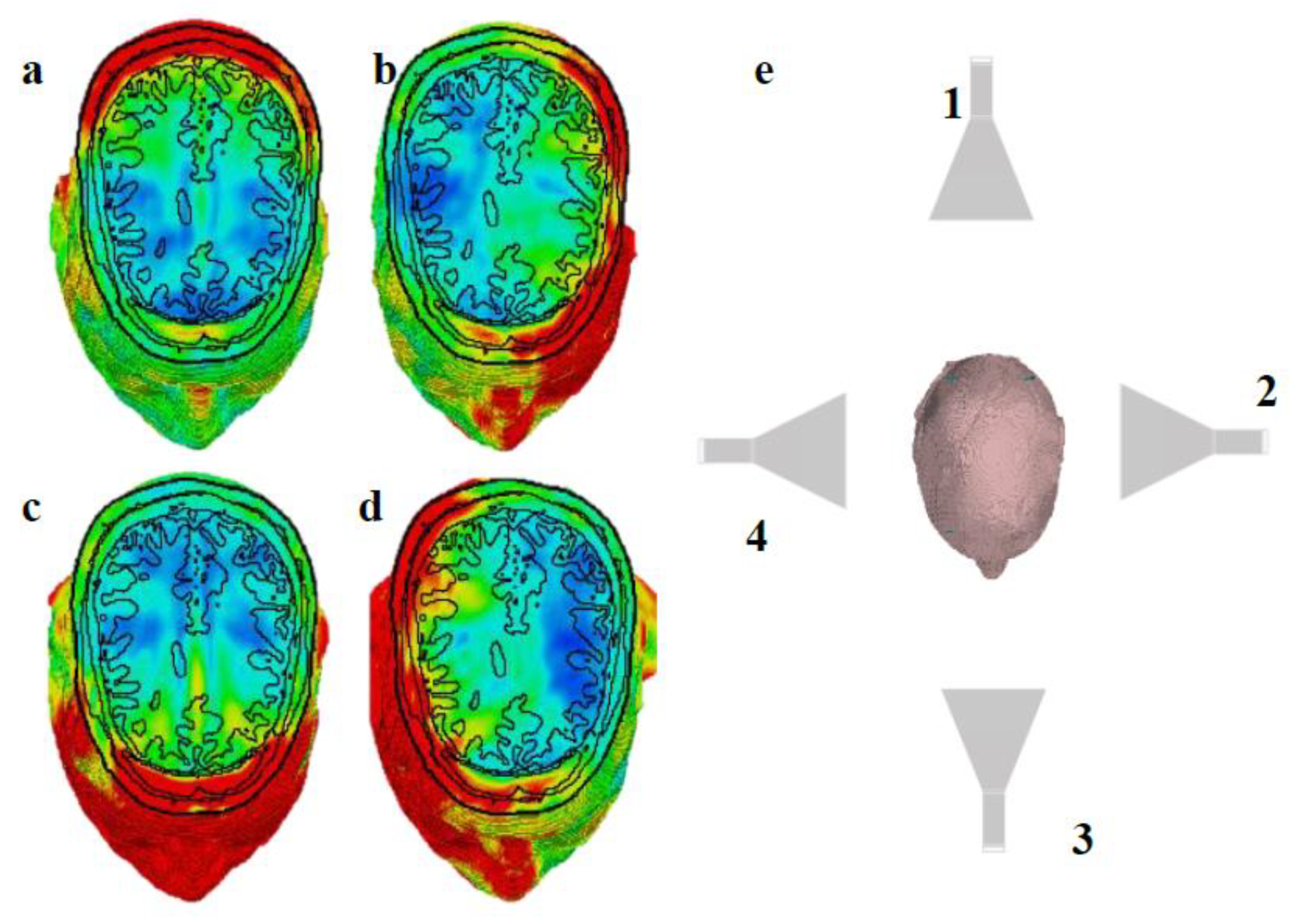
Our results also show early signs of steerability in the stimulation pattern. Specifically, simulations with a four-antenna configuration (Figure 11) demonstrated that modifying the output power of individual antennas can shift the location of maximum AM depth. In this setup, antennas 1 and 3 were operated at 2.45 GHz, while antennas 2 and 4 operated at 2.45 GHz + 100 Hz. By increasing the power of one antenna relative to the others, the peak AM depth moved accordingly, illustrating a clear directionality effect. These results are consistent with previous work (e.g., Reference [9]), which investigated the steering capabilities of implanted antenna arrays by adjusting the relative input amplitudes and phase.
It is pertinent to consider that in CST simulations, a balance exists between result accuracy and simulation duration. Reduced mesh dimensions enhance result accuracy but also lengthen simulation time. In this specific simulation, the finest mesh edge measured 0.66 mm, with negligible impact on results as the mesh size increased. Additionally, the simulations assumed a fixed distance and orientation between the antennas and the head model. However, in practical applications, patient motion—even when minimal—can alter the interference pattern and reduce targeting accuracy. Motion compensation techniques or real-time feedback systems will be essential for any clinical deployment. Furthermore, real-world environments introduce complexities not accounted for in this study, including multipath propagation, signal fading, environmental reflections, and potential interference with other medical equipment. These factors must be systematically addressed before translating this technology into clinical practice.
Despite these challenges, our findings suggest that non-contact, noninvasive deep brain stimulation using temporally interfering microwaves is a promising avenue for future neuromodulation research. The ability to focus energy at depth without surgical implantation could revolutionize treatment options for neurological disorders. As a next step, we plan to validate these findings through experimental studies using physical head phantoms. These experiments will help evaluate the real-world behavior of the system under controlled conditions. Additionally, future investigations will explore optimal frequency ranges and antenna configurations, as frequency selection directly impacts antenna size, penetration depth, and tissue interaction.
eclaration of interests
The authors declare that they have no known competing financial interests or personal relationships that could have appeared to influence the work reported in this paper.
- Marín, G., Castillo-Rangel, C., Salomón-Lara, L., Vega-Quesada, L.A., Calderon, C.Z., Borda-Low, C.D., Soto-Abraham, J.E., Coria-Avila, G.A., Manzo, J. and García-Hernández, L.I., 2022. Deep brain stimulation in neurological diseases and other pathologies. Neurology Perspectives, 2(3), pp.151-159. [CrossRef]
- Lee, D.J., Lozano, C.S., Dallapiazza, R.F. and Lozano, A.M., 2019. Current and future directions of deep brain stimulation for neurological and psychiatric disorders: JNSPG 75th Anniversary Invited Review Article. Journal of neurosurgery, 131(2), pp.333-342. [CrossRef]
- Raman, I.M., Gustafson, A.E. and Padgett, D., 2000. Ionic currents and spontaneous firing in neurons isolated from the cerebellar nuclei. Journal of Neuroscience, 20(24), pp.9004-9016. [CrossRef]
- TREFFENE, R.J., 1983. Interferential fields in a fluid medium. Australian Journal of Physiotherapy, 29(6), pp.209-216. [CrossRef]
- Grossman, N., Bono, D., Dedic, N., Kodandaramaiah, S.B., Rudenko, A., Suk, H.J., Cassara, A.M., Neufeld, E., Kuster, N., Tsai, L.H. and Pascual-Leone, A., 2017. Noninvasive deep brain stimulation via temporally interfering electric fields. cell, 169(6), pp.1029-1041. [CrossRef]
- Esmaeilpour, G. Kronberg, D. Reato, L. C. Parra, M. Bikson, Temporal interference stimulation targets deep brain regions by modulating neural oscillations, Brain Stimul. 14 (2021) 55–65. [CrossRef]
- B. Wang, A. S. Aberra, W. M. Grill, A. V. Peterchev, Responses of model cortical neurons to temporal interference stimulation and related transcranial alternating current stimulation modalities, Journal of neural engineering 19 (6) (2023) 066047. [CrossRef]
- Rampersad, S., Roig-Solvas, B., Yarossi, M., Kulkarni, P.P., Santarnecchi, E., Dorval, A.D. and Brooks, D.H., 2019. Prospects for transcranial temporal interference stimulation in humans: a computational study. NeuroImage, 202, p.116124. [CrossRef]
- Ahsan, F., Chi, T., Cho, R., Sheth, S.A., Goodman, W. and Aazhang, B., 2022. EMvelop stimulation: minimally invasive deep brain stimulation using temporally interfering electromagnetic waves. Journal of Neural Engineering, 19(4), p.046005. [CrossRef]
- N. Carnevale, M. Hines, The NEURON Book, Cambridge, UK: Cambridge University Press, 2006. [CrossRef]
- Huang, Y., Datta, A. and Parra, L.C., 2020. Optimization of interferential stimulation of the human brain with electrode arrays. Journal of neural engineering, 17(3), p.036023. [CrossRef]
- Hutcheon, B. and Yarom, Y., 2000. Resonance, oscillation and the intrinsic frequency preferences of neurons. Trends in neurosciences, 23(5), pp.216-222. [CrossRef]
- Mirzakhalili, E., Barra, B., Capogrosso, M. and Lempka, S.F., 2020. Biophysics of temporal interference stimulation. Cell Systems, 11(6), pp.557-572.
- Juutilainen, J. and de Seze, R., 1998. Biological effects of amplitude-modulated radiofrequency radiation. Scandinavian journal of work, environment & health, pp.245-254. [CrossRef]
- A. Vander Vorst, A. Rosen, Y. Kotsuka, RF/microwave interaction with biological tissues, John Wiley & Sons, 2006. doi:10.1002/0471752053.ch2.
- Pozar, D.M., 2011. Microwave Engineering. John Wiley & Sons. URL.
- T. Wagner, U. Eden, J. Rushmore, C. J. Russo, L. Dipietro, F. Fregni, S. Simon, S. Rotman, N. B. Pitskel, C. Ramos-Estebanez, et al., Impact of brain tissue filtering on neurostimulation fields: a modeling study, Neuroimage 85 (2014) 1048–1057. doi:10.1016/j.neuroimage.2013.06.079.
- Xiao, Q., Zhong, Z., Lai, X. and Qin, H., 2019. A multiple modulation synthesis method with high spatial resolution for noninvasive neurostimulation. PloS one, 14(6), p.e0218293. doi: 10.1371/journal.pone.0218293.
- A. L. Hodgkin, A. F. Huxley, A quantitative description of membrane current and its application to conduction and excitation in nerve, J. Physiol. 117 (1952) 500–544. doi:10.1113/jphysiol.1952. sp004764.
- https://space.mit.edu/RADIO/CST_online/mergedProjects/3D/ common_tools/common_tools_biomodels.htm#Voxel_Famim.
- https://space.mit.edu/RADIO/CST_online/mergedProjects/3D/common_tools/common_tools_human_material_macro.htm.
- https://www.fcc.gov/general/body-tissue-dielectric-parameters.
- Chou, C.K., Bassen, H., Osepchuk, J., Balzano, Q., Petersen, R., Meltz, M., Cleveland, R., Lin, J.C. and Heynick, L., 1996. Radio frequency electromagnetic exposure: Tutorial review on experimental dosimetry. Bioelectromagnetics: Journal of the Bioelectromagnetics Society, The Society for Physical Regulation in Biology and Medicine, The European Bioelectromagnetics Association, 17(3), pp.195-208. doi:10.1002/(SICI) 1521-186X(1996)17:3<195::AID-BEM5>3.0.CO;2-Z.
- International Commission on Non-Ionizing Radiation Protection, 2020. Guidelines for limiting exposure to electromagnetic fields (100 kHz to 300 GHz). Health physics, 118(5), pp.483-524. doi:10.1097/HP.0000000000001210.
- https://www.3ds.com/products/simulia/antenna-magus.
- R. B. Keller, Design for Electromagnetic Compatibility–In a Nutshell: Theory and Practice, Springer Nature, 2023. doi:10.1007/978-3-031-14186-7.
Figure 1.
Simulation space in CST environment, human head in front of two horn antennas.
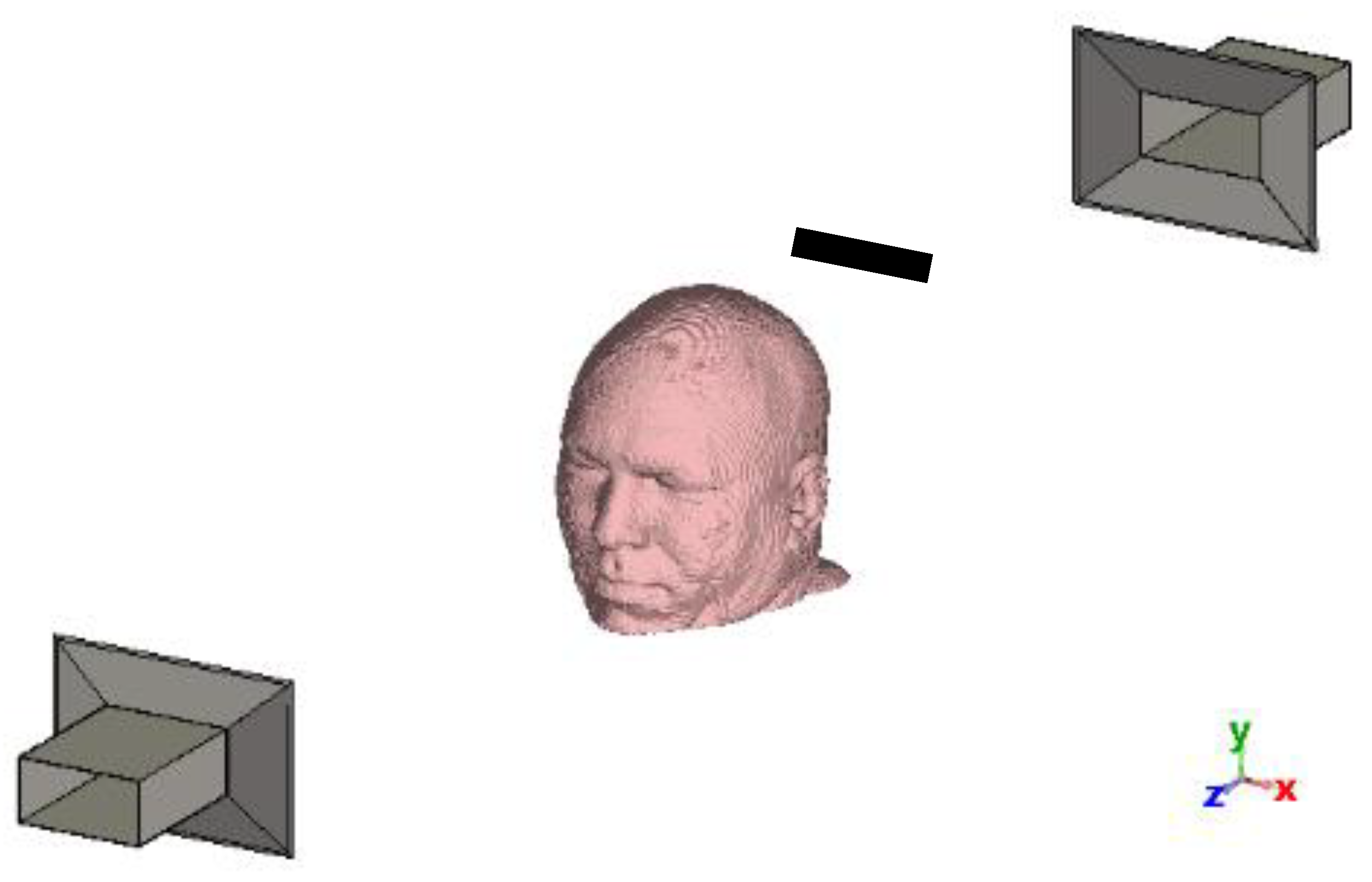
Figure 2.
Interfering electric fields, A. one-dimensional interference B. 3D interference.
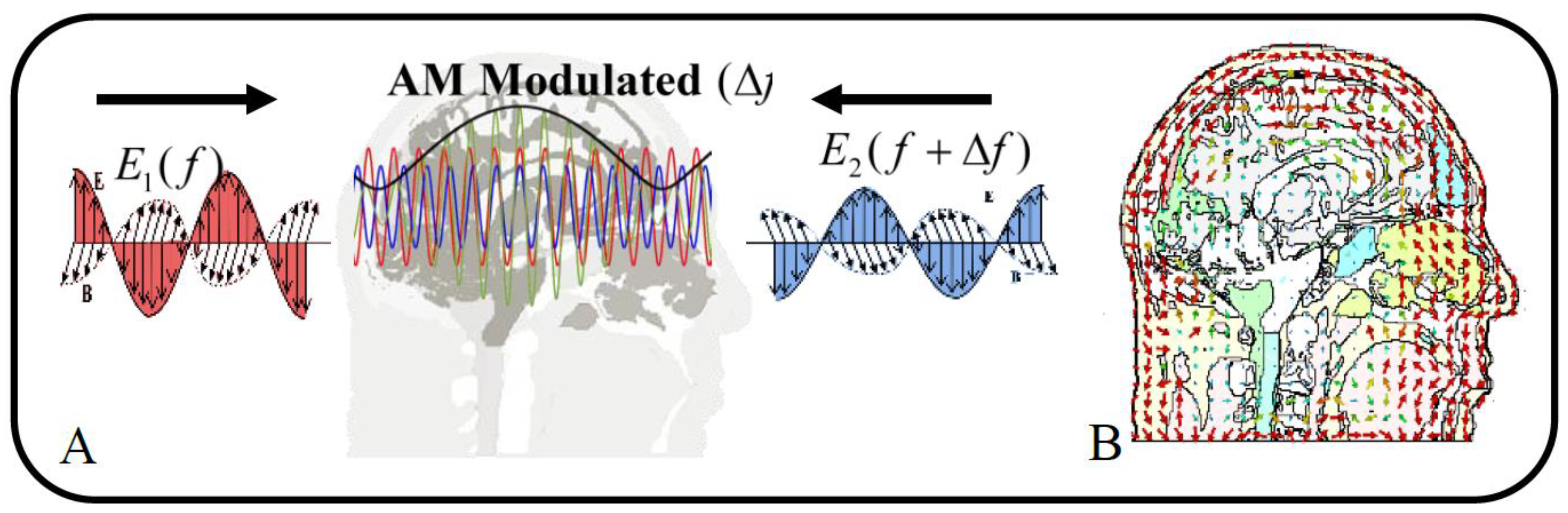
Figure 3.
Neuron as a single compartment soma.
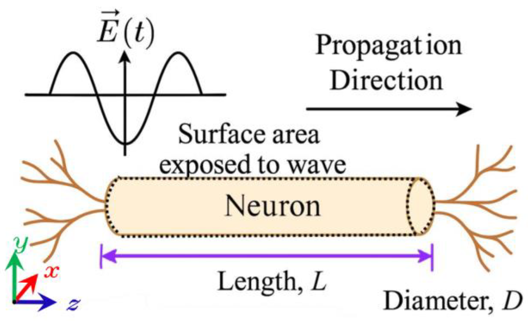
Figure 4.
ICNIRP (2020) local exposure thresholds [24].
Figure 4.
ICNIRP (2020) local exposure thresholds [24].
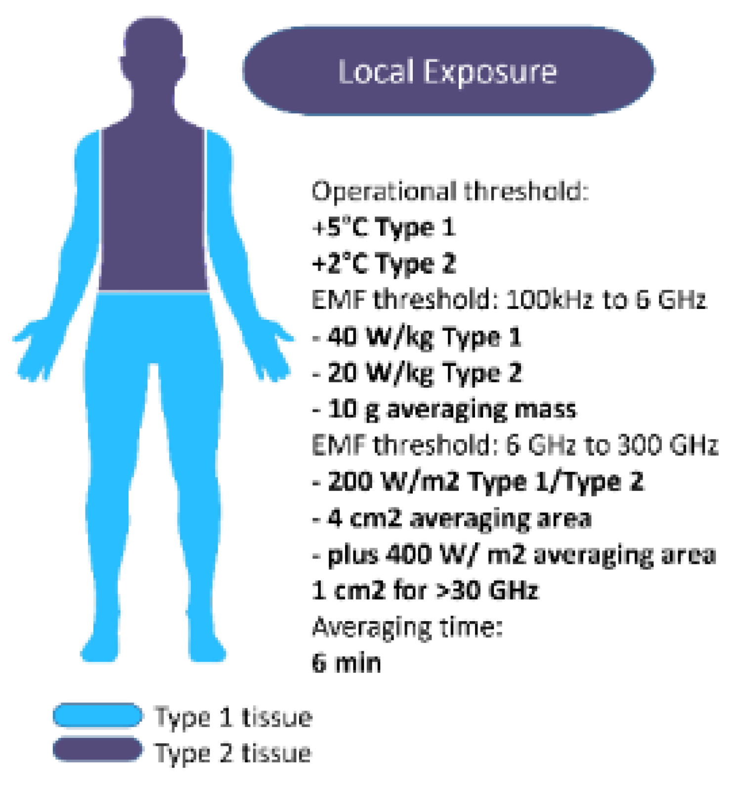
Figure 5.
illustrates the precise placement of the probes at all four levels of the head. It is important to note that some probes are positioned outside of the brain, and only the results from those probes located within the brain have been included in the simulations. Specifically, 53 probes were utilized at level 1, while levels 2, 3, and 4 employed 65, 60, and 32 probes, respectively, resulting in a total of 210 probes placed inside the brain. To refer to each probe, we will indicate its number based on its position in the x and z axes, while also specifying the level it corresponds to. For example, the blue probe depicted in Figure 5 will be identified as Probe
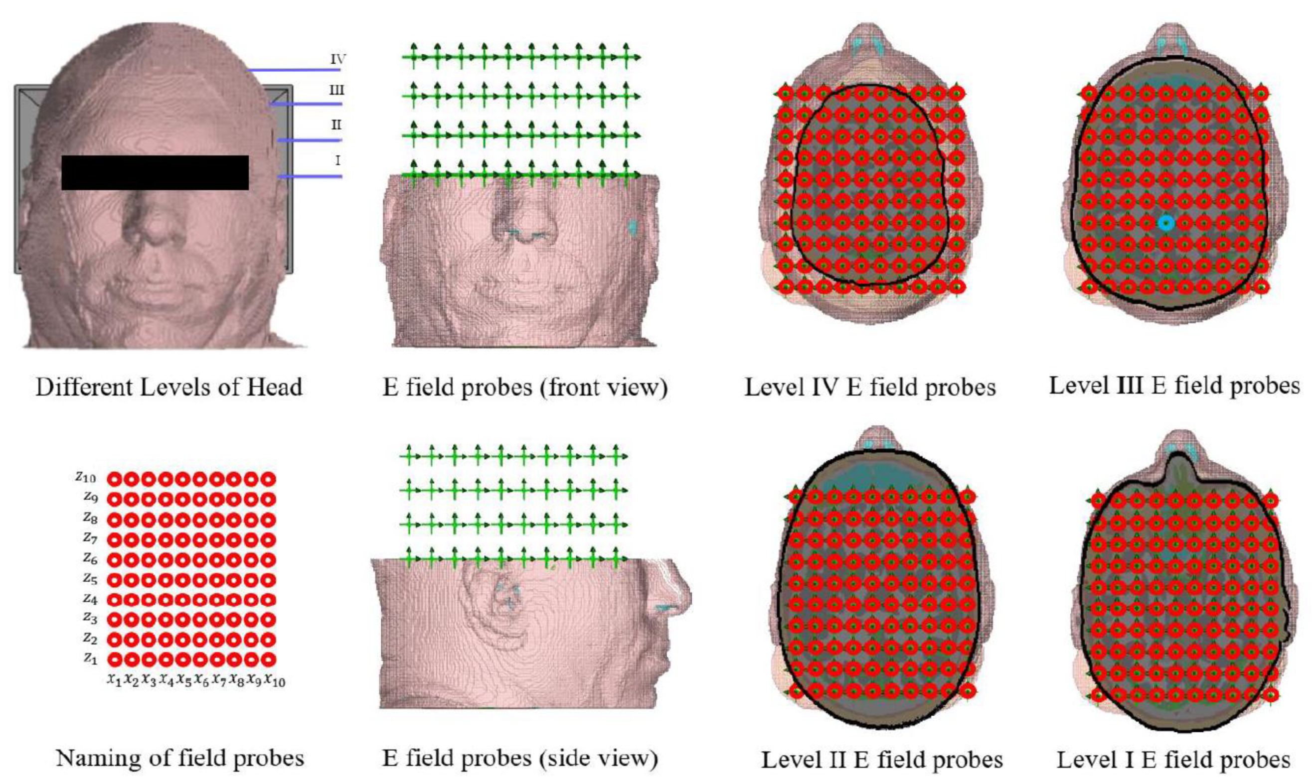
Figure 6.
CST output for the maximum values of the absolute magnitude of the electric field and the y-component of the electric field for all four levels of Figure 5.
Figure 6.
CST output for the maximum values of the absolute magnitude of the electric field and the y-component of the electric field for all four levels of Figure 5.
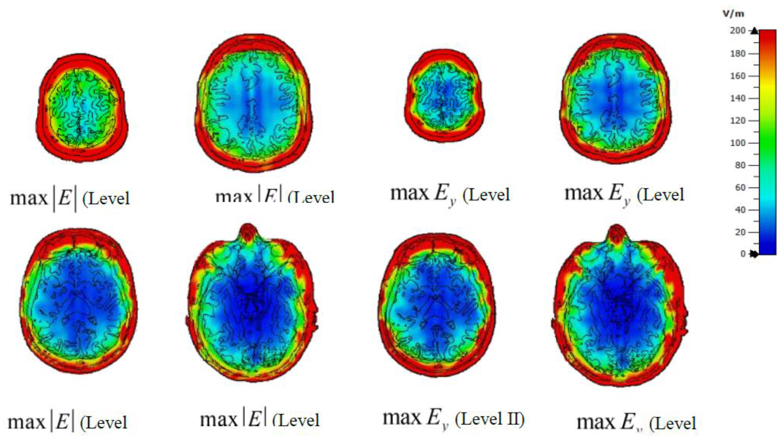
Figure 7.
y-component of the AM intensity (both antennas transmit at 30 kW).
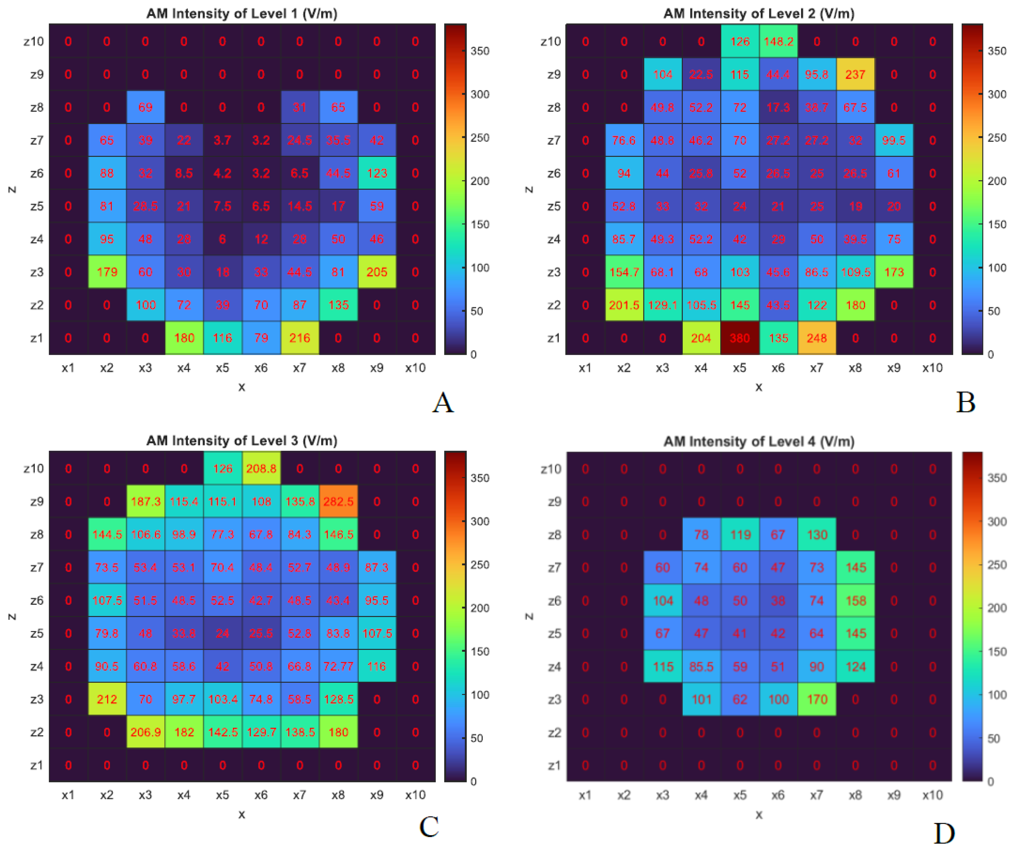
Figure 8.
y-component of the AM depth (both antennas transmit at 30 kW).
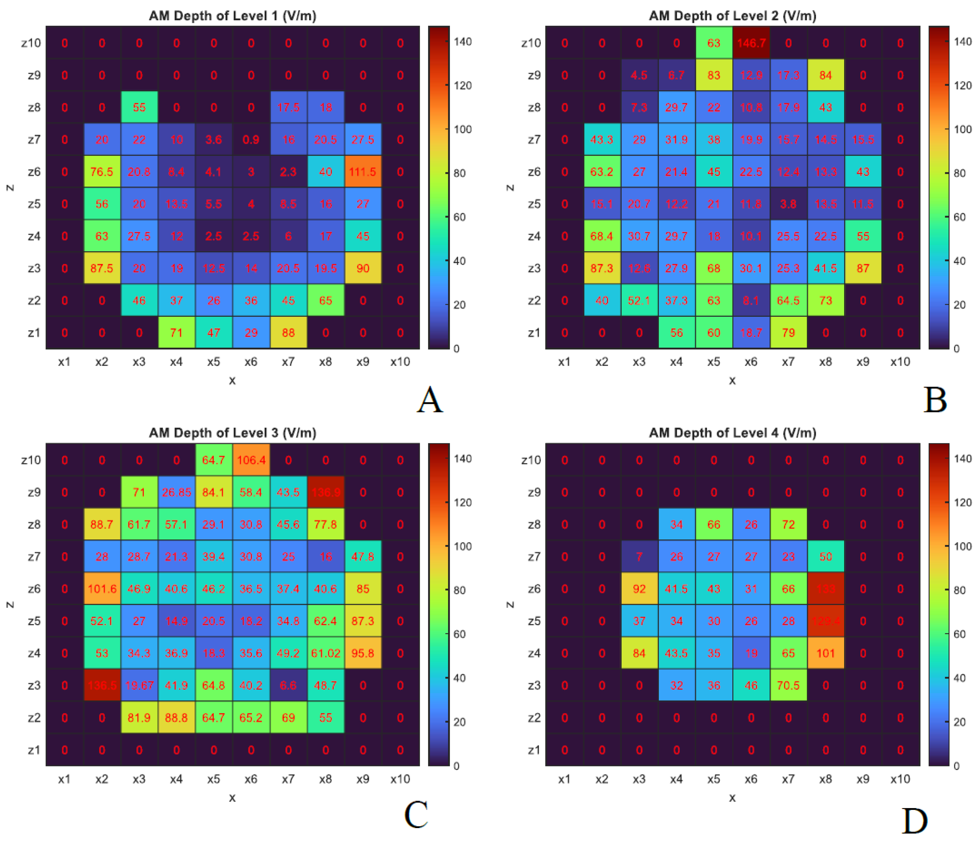
Figure 9.
Number of action potentials generated by the Hodgkin-Huxley neuron model across all four levels and probe locations for different antenna output powers.
Figure 9.
Number of action potentials generated by the Hodgkin-Huxley neuron model across all four levels and probe locations for different antenna output powers.
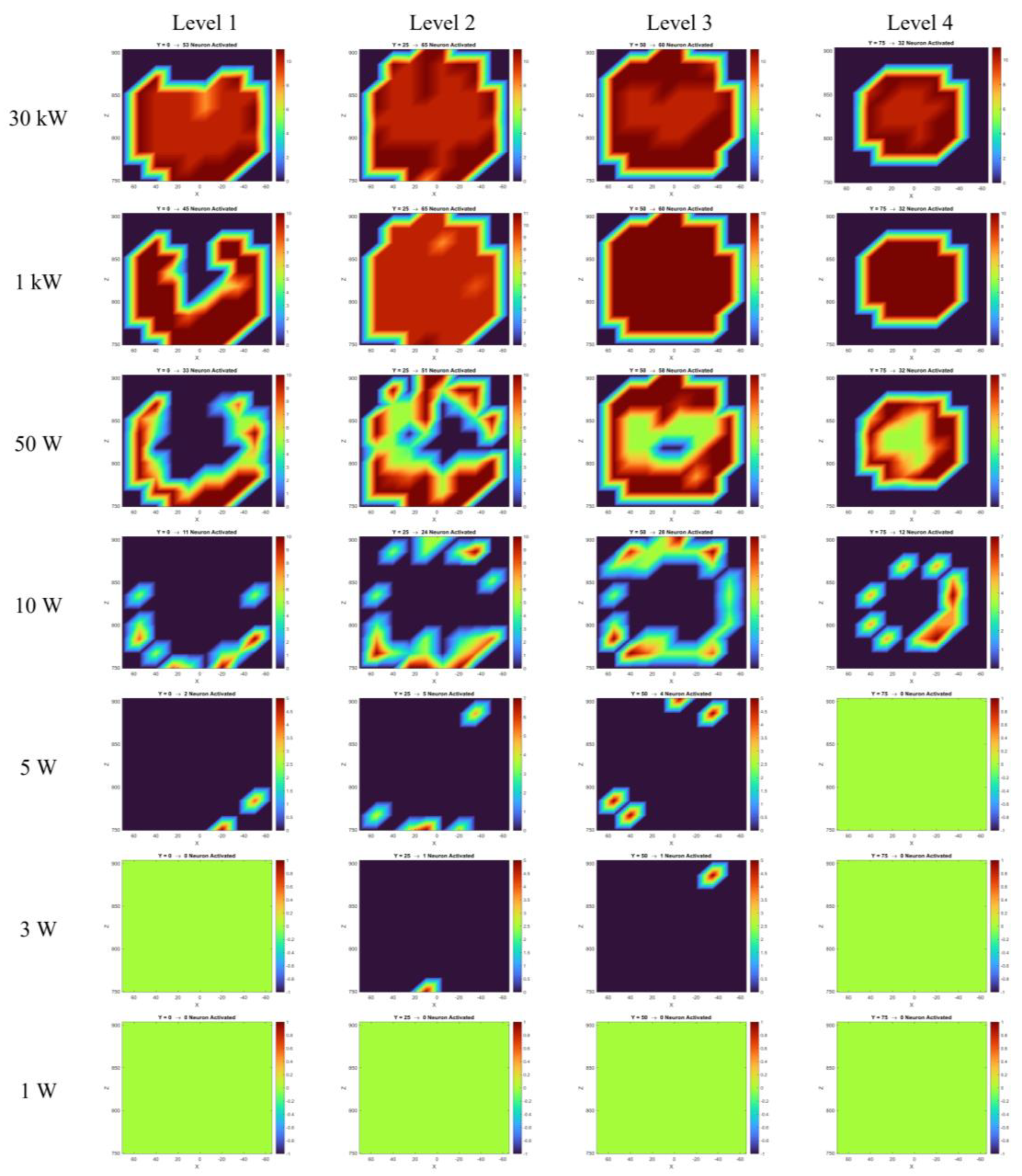
Figure 10.
Number of activated neurons at each level as a function of the transmitted power (assuming both antennas operate at the same output power).
Figure 10.
Number of activated neurons at each level as a function of the transmitted power (assuming both antennas operate at the same output power).
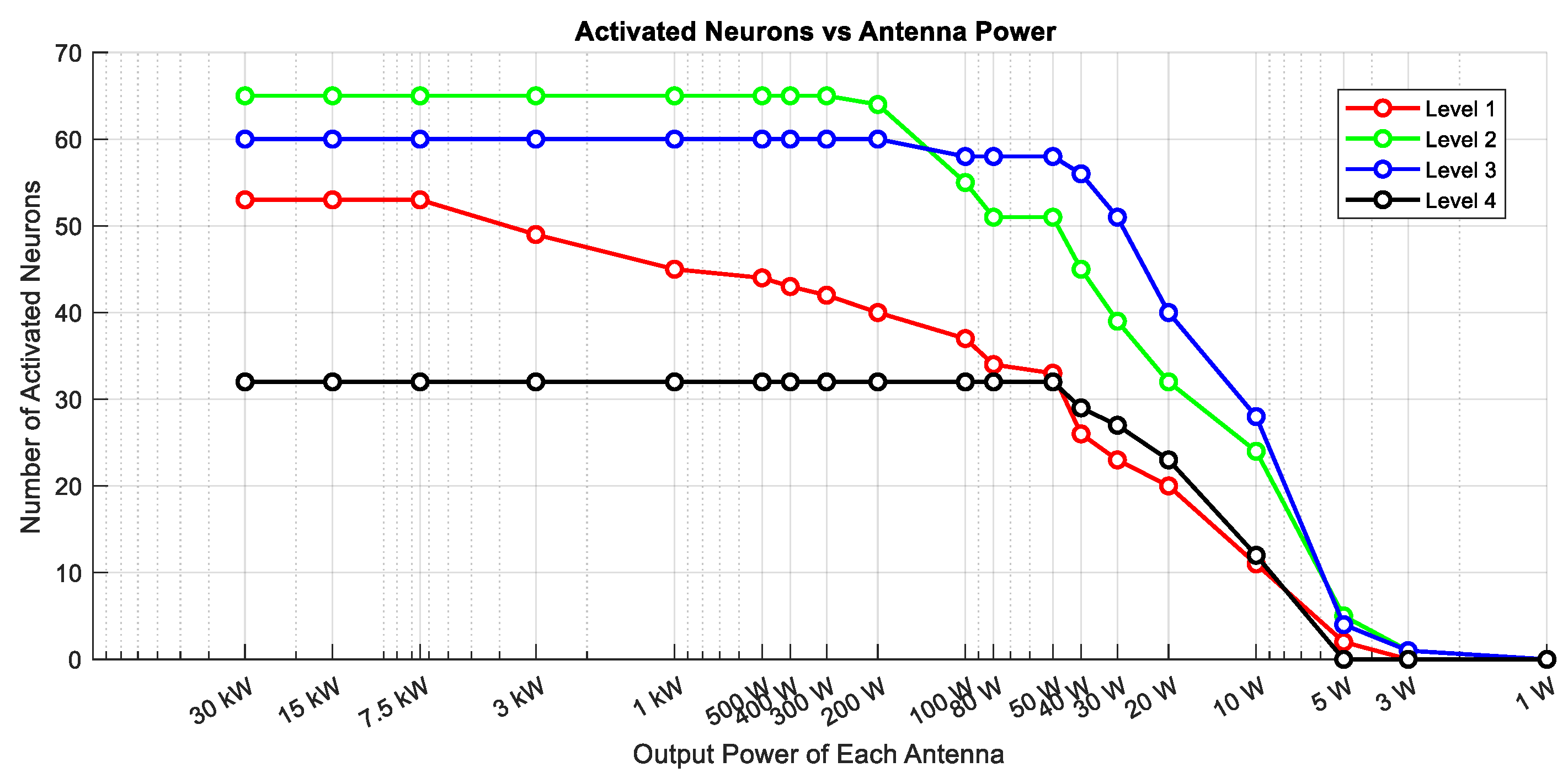
Figure 11.
evel III stimulation site’s steerability. A: The electric field’s intensity when antenna 1’s output power is five times that of the other antennas. B: The electric field’s intensity when antenna 2’s output power is five times that of the other antennas. C: The electric field’s intensity when antenna 3’s output power is five times that of the other antennas. D: The electric field’s intensity when antenna 4’s output power is five times that of the other antennas. E: Arrangement of antennas and their position relative to the head (sizes and proportions are not precise.).

| Name | Value & unit | Description |
|---|---|---|
| 1 μF/cm2 | Membrane capacitance | |
| 120 mS/cm2 | Sodium conductance | |
| 36 mS/cm2 | Potassium leak conductance | |
| 0.3 mS/cm2 | Leak conductance | |
| 45 mV | Sodium reversal potential | |
| -82 mV | Potassium reversal potential | |
| -59 mV | Leak reversal potential | |
| L | 9.6 μm | Length of soma |
| D | 9.6 μm | Diameter of soma |
Table 2.
The dielectric properties of the human head at 2.45 GHz frequency [18].
Table 2.
The dielectric properties of the human head at 2.45 GHz frequency [18].
| Tissue | Permittivity () | Conductivity () |
|---|---|---|
| Blood | 58.263756 | 2.544997 |
| Bone Cortical | 11.381223 | 0.394277 |
| Cartilage | 38.771160 | 1.755682 |
| Cerebellum | 44.803696 | 2.101270 |
| Cerebro Spinal Fluid | 66.243279 | 3.457850 |
| Dura | 42.035004 | 1.668706 |
| Eye Tissue(Sclera) | 52.627628 | 2.033048 |
| Fat (Mean) | 10.820482 | 0.267954 |
| Grey Matter | 48.911255 | 1.807664 |
| White Matter | 36.166599 | 1.215008 |
| Avg. Brain | 42.538925 | 1.511336 |
| Avg. Skull | 14.965101 | 0.599694 |
| Skin (Dry) | 38.006660 | 1.464073 |
| Avg. Muscle | 53.573540 | 1.810395 |
Table 3.
Average permittivity, conductivity, and density for brain, skull, and muscle at 2.45 GHz frequency [18].
Table 3.
Average permittivity, conductivity, and density for brain, skull, and muscle at 2.45 GHz frequency [18].
| Tissue | Density () | Permittivity () | Conductivity () |
|---|---|---|---|
| Avg. Brain | 1030.0 | 42.538925 | 1.511336 |
| Avg. Skull | 1850.0 | 14.965101 | 0.599694 |
| Avg. Muscle | 1040.0 | 53.573540 | 1.810395 |
Table 4.
Antenna specifications.
| Description | Value |
|---|---|
| Centre frequency | 2.45 GHz |
| Gain | 9.7 dBi |
| Width of waveguide section | 96.06 mm |
| Height of waveguide section | 48.03 mm |
| Length of waveguide section | 122.4 mm |
| Aperture width | 175.2 mm |
| Aperture height | 118.4 mm |
| Length of flare section | 567.2 μm |
Disclaimer/Publisher’s Note: The statements, opinions and data contained in all publications are solely those of the individual author(s) and contributor(s) and not of MDPI and/or the editor(s). MDPI and/or the editor(s) disclaim responsibility for any injury to people or property resulting from any ideas, methods, instructions or products referred to in the content. |
© 2025 by the authors. Licensee MDPI, Basel, Switzerland. This article is an open access article distributed under the terms and conditions of the Creative Commons Attribution (CC BY) license (http://creativecommons.org/licenses/by/4.0/).
Copyright: This open access article is published under a Creative Commons CC BY 4.0 license, which permit the free download, distribution, and reuse, provided that the author and preprint are cited in any reuse.


