Submitted:
22 May 2025
Posted:
23 May 2025
You are already at the latest version
Abstract
The basic theoretical properties of the approximate symmetric chordal metric (ASCM) for two real or complex numbers is studied, and reliable, accurate and efficient algorithms are proposed for its computation. ASCM is defined as the minimum between the moduli of the differences of the two numbers and of their reciprocals. It differs from chordal metric by including the modulus of the difference of the numbers. Is is shown that ASCM is not a true mathematical distance, but a useful replacement for a distance in some applications, such as block diagonalization of matrix pencils. A factored representation of the modulus of complex numbers is introduced, which allows to obtain very accurate results for the entire range of the floating point number system of a computer. Two different ways to evaluate the distance between the reciprocals of the given numbers are described. The algorithms can be easily implemented on various architectures and compilers. Extensive numerical tests have been performed to assess the performance of the associated implementation. The results have been compared to those obtained in MATLAB, but with appropriate modifications for numbers very close to the bounds of the range of representable values, where usual formulas give wrong results.
Keywords:
algorithm
; block diagonalization
; software
; chordal metric
1. Introduction
The approximate symmetric chordal metric for two real or complex numbers is defined by
It differs from the Euclidean distance by also considering the absolute difference of the reciprocals of the given numbers. As shown in Remark 1, Section 2, d in (1) is not a true mathematical distance, but a useful replacement for a distance in some applications. In particular, it can be used even if one number, say , is infinite; as shown in Theorem 1 (vi), the result is finite if .
There are quite many references on chordal metric, but no references to the approximate symmetric chordal metric could be found. In one of the early papers on chordal metric, Klamkin and Meir [1] have shown that a normed linear space is Ptolemaic if and only if it is symmetric, and that the chordal metric, defined using that space norm, , for x, , satisfies the triangle inequality. A main approach to define the chordal metric is via the stereographic projection, e.g., [2,3,4]. Let be the Riemann sphere with diameter 1 and center in , defined by . The -plane tangent to in the origin can be seen as the complex z-plane . Let ı be the purely imaginary unit. Stereographic projection is the map defined by the intersection of the chord with , where is identified with in the -plane, and is the north pole of . Let be a parametrization of the line from N to z, with ; clearly, and ; hence, the intersection is for , and satisfies the equation . The solutions are , corresponding to N, and , giving The stereographic projection of to is defined by
If is the Euclidean metric in and that on inherited from , then it can be shown that,
which is the chordal metric of . Clearly, . If , then . This way, becomes a map from the extended complex plane to . Note that if z, . The triangle inequality is satified by , being implied by that inequality for Euclidean distance in ; therefore, chordal metric is indeed a distance. If , then the formula becomes . If a Riemann sphere with unit radius and center in the origin is used, then the formulas for the chordal metric should be multiplied by 2 [3,5]. It is also mentioned in [3] that if and .
Several authors present theretical results and various applications of the chordal metric. Rainio and Vuorinen [4] use (2) to identify some cases where the distortion caused by symmetrization of a quadruple of points or objects, mapped by a Möbius transformation, can be measured in terms of the Lipschitz constant of this transformation in the Euclidean or the chordal metric. Álvarez-Tuñón et al [6] investigate various pose representations and metric functions in visual odometry networks, and show that the chordal distance ensures better generalization and faster convergence of the network parameters than distances measured by Euler angles or quaternions; this is useful to estimate the change of position, e.g., of robots, relative to a starting location, based on data from motion sensors. However, this paper uses the chordal distance between two rotations, and , defined as , where I is the identity matrix of order 3 and F denotes the Frobenius norm. Xu et al [7] provide explicit expression and sharper bounds of the chordal metric between generalized singular values of Grassmann matrix pairs. A constrained optimization problem of the form , where is the set of unitary matrices, is studied and its optimal solution is given. The results are applied to comparative analysis of gene mRNA expression data for mice macrophage under different conditions. Sun [8] considers the generalized singular values (GSVD) when , where A and B are complex and , respectively. Then, any pair satisfying and is a singular value, . For such a case, it is difficult to investigate the perturbation of singular values. It is shown that when [ ] is strongly perturbed, the singular values are insensitive to perturbations in the elements of A and B, if the chordal metric is used to describe such perturbations. Sasane [2] defines an abstract chordal metric on linear control systems described by their transfer functions and shows that strong stabilizability is a robust property in this metric. In [9], a refinement of this metric for standard classes of stable transfer functions is introduced.
A common application of the approximate symmetric chordal metric is related to ordering the eigenvalues of a matrix or matrix pencil, according to their pairwise distances measured using (1). For generalized eigenvalue problems, i.e., for matrix pencils, some eigenvalues may be infinite. Ordering (generalized) eigenvalues is very important in many applications of numerical linear algebra, control theory and other domains. For instance, it is essential for computing invariant or deflation subspaces of matrices or matrix pencils, respectively. A more general application of the approximate symmetric chordal metric is for computing the block-diagonal form for matrices or matrix pencils [10], especially for large order problems. This form is useful for finding reciprocal condition numbers for eigenvalues and related eigenspaces, as well as for fast computation of matrix functions or of the responses of linear time invariant standard or descriptor systems. Assuming that the matrix (pencil) is already reduced to a (generalized) Schur form [11], an essential part of the computations is the solution of a (generalized) Sylvester equation. This part involves non-unitary transformations. To ensure an acceptable numerical precision, the solution elements should be bounded. Specifically, if any element of the solution exceeds a given threshold , then the process is stopped, and an enlarged Sylvester equation is tried to be solved. If many failed attempts are necessary, then the computational effort might be unacceptably high, especially for large order problems. A clever strategy for ordering the eigenvalues of the matrix (pencil) might reduce the number of failed trials, since the magnitude of the solution is influenced by the sensitivity of the spectrum associated to the current block that should be separated. The sensitivity of eigenvalue problems and related topics are investigated in [11,12,13,14,15,16]. Efficient and reliable implementations of the theoretical results are available in the LAPACK package [17] and in interactive environments like MATLAB [18] or Mathematica [19]. The eigenvalues can be ordered based on their pairwise “distances” measured by (1). These eigenvalue applications do not need the triangle inequality be satisfied. But it is important that close eigenvalues be included in the same cluster. The use of the min function in (1) will choose an eigenvalue to be added to a cluster containing a value if either or is smaller than a given threshold. An approach based on the chordal metric cannot do that. Clearly, , if and . Therefore, in such a case, coincides to the chordal metric in [1], and is often quite close to the usual definition of the chordal metric (2). The distance is not directly taken into account, although it could be smaller than .
This section is ended by some issues, needed in the sequel, concerning the floating point system of computers. For technical convenience, will denote the real numbers field extended by the ∞ and symbols, and similarly for . This is useful, since practical calculations with computer software like MATLAB encounter such situations.
A complex "number" , with , is infinite if and/or . Otherwise, a is finite. Consider two finite complex numbers, , . It is assumed that and , , are in the range of the floating point system of a computer, hence and are (approximately) representable by their real and imaginary parts. Therefore, , , where K is the maximum representable number, defined by
where b is the base of the numeral system, is the maximum exponent, and is the smallest distance between two representable numbers (also called the relative machine precision). In a commonly used binary double precision floating point system, , , (or for machines with proper rounding in the addition operation), and , where t is the number of base digits in the mantissa, i.e., the fractional part of the representation in base b. Note that the result of evaluating K as in (3) might not be representable on such a computing machine, since it could exceed K; but evaluating will not overflow. The number is called precision. On the machine considered above, with proper rounding, , but .
Clearly, not all real or complex numbers can be represented on a digital computer, since the floating point system deals with rational approximations of the numbers in the range . If an arithmetic operation would produce a result outside this range, that fact is called overflow. Compilers and interactive environments may represent such a result as ±Infinity or ±Inf, and if this happens in a sequence of computations, the final result might be completely wrong. Therefore, overflows should be avoided. On the other hand, very small (in magnitude) numbers may also be not representable, and if this is the case for the result of a mathematical operation, it may be set to zero. This is the counterpart of an overflow, and it is called underflow, but it is not as severe as overflows. The underflow threshold is defined by , where is the minimum exponent before underflow. For the machine considered above, . Many computer systems allow for gradual underflow, i.e., they may also use numbers less than k, in the range . For this reason, the availability of gradual underflow will be assumed in this paper.
Algorithms for discovering the properties of the floating point arithmetic, like in [20,21], are implemented, e.g., in the SLAMCH and DLAMCH routines of the LAPACK package [17], for single and double precision computations, respectively. A special function is used to ensure that all relevant values are stored, and not held in registers, or not affected by compiler optimizations.
In the sequel, there will be no distinction between a number and its floating point representation. Note that the assumption that , , does not imply that and . If and , then , which is not representable. The specific case of our application allows to work with a factored form of and .
The rest of the paper is organized as follows. Section 2 investigates the properties of the approximate symmetric chordal metric, while Section 3 presents reliable, accurate, and efficient algorithms for its computation. Section 4 discusses the numerical results obtained using a careful implementation of these algorithms. Section 5 summarizes the conclusions.
2. Basic Properties of the Approximate Symmetric Chordal Metric
In some applications using (approximate symmetric) chordal metric, and/or or the terms in (1) may not be numbers, but 0/0 or . For instance, some eigenvalues of singular matrix pencils are 0/0. Moreover, even for nonsingular matrix pencils, some eigenvalues are infinite, but in some routines, e.g., as those in LAPACK [17], the eigenvalues are in fact ratios of pairs of numbers, and , with possibly 0; if in (1), for , , then the first term of the min function in (1) is . In such cases, it is necessary to use special computer rules for mathematical operations, as shown below.
A Not-a-Number entity is represented by NaN in compilers and interactive environments like MATLAB.
Definition 1.
(Basic operations withNaNs and numbers)
- NaN ∘ a = NaN, NaNa = NaN, aNaN = NaN, where , × and / are the multiplication and division binary operations, and .
- NaN ∘ a = NaN ∘ βı, NaNa = NaN + NaNı, aNaN = NaN + NaNı, for .
- |NaN| = NaN, min(NaN, a) = a, max(NaN, a) = a, for .
For convenience, conventions like and are adopted here; these conventions make sense thinking in terms of limits, for intance, , for x taking positive of negative values only, respectively.
The next theorem shows the basic properties of the approximate symmetric chordal metric. The results are true even if and/or , , are infinite.
Theorem 1
- (i)
- ;
- (ii)
- , ;
- (iii)
- , ;
- (iv)
- if and are infinite;
- (v)
- ;
- (vi)
- , if is infinite, ;
- (vii)
- if and or , or both, are finite.
Proof.
The symmetry property (i) follows immediately from (1). Property (ii) holds since the second argument of the min function in (1) is infinite, hence, , and ; clearly, (ii) is also true for , , , or , with and finite, since then too. (For convenience, when appears, the other two cases, with either or finite, will not be mentioned, but the related property is also true for these cases.) From (1), property (iii) holds for finite a; if or , then NaN, , and , according to the third item in Definition 1. If or and , (iv) has been proved in (iii), while if , or , where is the complex conjugate of a, then (iv) follows, since and . Clearly, from (iii) and (iv) it follows that implies . Conversely, if , then either , if and are finite, or , if and are infinite, so . These two facts prove the identity property (v). If is finite, (vi) follows since and ; (vi) is also true if or since, from (iv), . If , then (vi) holds since and , so . If and are finite and distinct, both terms of min are strictly positive, which prove (vii); if is finite, but is infinite, then is infinite, hence, by (vi), . The symmetry property makes the result true also for infinite and finite. □
Remark 1.
Theorem 1 proves that three properties of a distance or metric, namely, symmetry, identity and non-negativity, are satisfied by . But it is easy to verify that the fourth needed property, the triangle inequality, does not hold for (1), therefore the inequality , is not true in general, for . Consequently, is not a distance or metric function. Moreover, the approximate symmetric chordal metric does not satisfy a scaling property, that is, differs, in general, from , with . For instance, for , , and , and , but for , . The ratios in the two cases are 0.5 and 0.25, respectively, not 2 and 4. Such scaling property holds for and for , but not necessarily for their minimum.
In order to be able to accurately work on the entire range of representable complex numbers, a special representation of the absolute value is used, as defined below.
Definition 2.
(Factored representation of the absolute value of a complex number a)
Let with and . Let , , and . Then is called the factored representation of .
From Definition 2 it follows that , since if , if , and values will imply . Factored representation is useful when M is vey close to or coincides to K. In such a case, the product could exceed K, and then cannot be computed. Still, its factors can be used in all computations needed for obtaining the approximate symmetric chordal metric.
3. Algorithms for Computing the Approximate Symmetric Chordal Metric
A conceptual algorithm is first presented, and then it will be detailed. The symbols ∧, ∨ and ¬, used in the algoriths and their description below, are the binary logical operators AND, OR and NOT, respectively. Moreover, and denote the sets of complex and real representable numbers, respectively. However, the algorithms below will also correctly work for and/or set to ±Infinity or ±Infinity ±Infinityı, if the IEEE arithmetic is available on the computer. Although the computational problem for approximate symmetric chordal metric looks mathematically very simple, a reliable, accurate, and efficient implementation needs a thorough analysis. These desirable properties are supported by careful consideration of all possible special cases and lower level algorithms. Efficiency can be measured by an estimate of the number of floating point operations, or flops, which have been used especially for numerical linear algebra algorithms [11,22]. One definition says that a flop consists in an addition, a multiplication and few memory addresses. Another definition considers each addition, subtraction, multiplication and division of two floating point numbers as a flop. This is suitable in the paper context.
3.1. Conceptual Algorithm
In the first part of the Algorithm chordal, the value of is computed for special cases. If the maximum absolute value, M, of the real and imaginary parts of and , is zero, or if , then , according to (iii) in Theorem 1. Otherwise, if , which implies that , then , using (i) and (ii). Similarly, if , then . The absolute values , for and , are computed by a lower level algorithm, called absa, introduced in the next subsection. Algorithm absa needs on input the auxiliary parameters M and or , set in Algorithm chordal, using .
Another special case is when one of the numbers or is negligible compared to the other. Then, as shown below, can be found using , , or both. Detecting this situation involves the logical variable , with . See Remark 2 below. If f is true, then it is easier to obtain the terms and of d in (1). Specifically, if and , , it follows that: if , then ; else if , then ; else . The tests involving m and M are motivated by the following reason: implies that is of the order of M, and is of the order of ; if , and have comparable values, and d should be found as ; if m is smaller enough than , then and so . Similarly, if m is larger enough than , then , and so . The bounds 0.1 and 1.1 have been found after few trials, so that all tests returned the correct results. Note that, in the discussion above and in Algorithm chordal, the product is not used, since it may overflow if and are close to K.
Remark 2.
Using Definition 2, the absolute value of , , can be expressed as , where . Indeed, , if and , if . Clearly, if , then . This factored form of is valid even if , when the factors cannot be multiplied without producing an overflow. If , it follows that
since and . Therefore, if is negligible compared to , the same is true for and . The last inequality in (4) assumes that the base of the floating point system is . For the previous paragraph, and .
If no special case appears in Algorithm chordal, it follows that and are nonzero, distinct and relatively “close” to each other, in the sense that . This is the general case, for which it is necessary to compute and . Finally, . These more involved computational steps of the conceptual algorithm are detailed in the next subsections.
An account of the needed computations can be given here for the part involving special cases, but additional details, including those for general case, will be available in the remaining subsections of this section. At the beginning of Algorithm chordal, the computation of the absolute values for four real scalars, as well as three standard max operations (i.e., with two arguments) are needed, for getting , , and M. If or , which requires three comparisons of real scalars, the result is . Otherwise, if , then , with and or ; each of these cases needs an evaluation of one norm (either of or of ); in addition, a division and two tests are needed to set , . If for , the special case when or is tried. The initialization of this pseudocode segment involves a standard min operation, two divisions and a comparison, setting the value of the logical variable f. If and , then there are three cases: if , then ; else, if , then , for ; else, . Hence, in addition to the inialization part, the computations involve three or four tests, one or three divisions, one or two evaluations of the absolute value, and—for the third case—one standard min operation.
| Algorithm 1 chordal computes ASCM for two complex numbers |
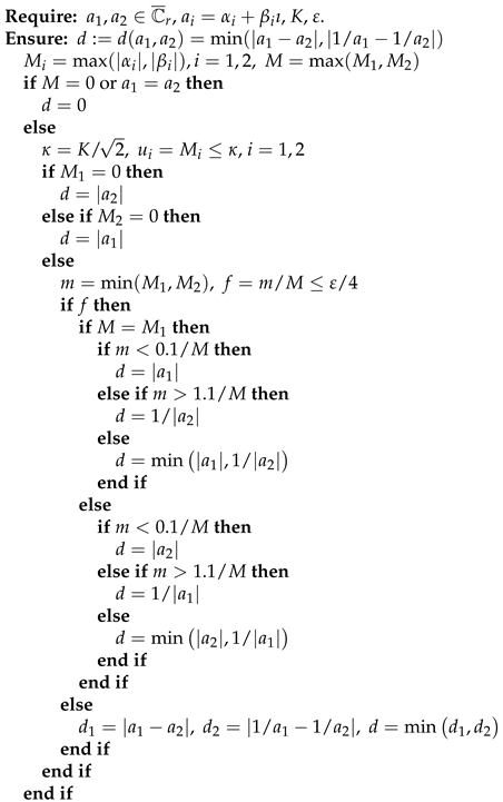 |
3.2. Computation of ,
If the magnitude of the real and imaginary parts of are close to the maximum representable number, K, then may overflow. For the computation of the approximate symmetric chordal metric d, it is possible to use the factored form of , using M and given in Definition 2, namely, , and , with .
For example, for , the direct computation of abs(a) in MATLAB gives Inf, the machine infinity, while can very accurately be represented by the product factors and . Actually, abs(a), i.e., , is also evaluated internally in a factored form in MATLAB or in other available routines, like DLAPY2 from LAPACK [17], but the result is returned as a product, . However, in most cases, is far from K, and always using the factored form would involve some unnecessary computations. For efficiency, a bound is used to detect a case when the factored form might be needed. Specifically, if , with defined in Algorithm chordal, then one can safely use abs(a) in MATLAB, or DLAPY2 from LAPACK to obtain . Otherwise, it is safer to employ the factored form. Since is a conservative bound, it is possible that be representable. The needed test is included in the Algorithm absa, listed below, and explained in Remark 3; the logical variable u, externally initialized to true if , is updated internally as .
| Algorithm 2 absa computes the modulus (or its factored representation) of a complex number |
|
If on entry, Algorithm absa needs in principle to square two real numbers and make an addition and a square root. This computation can be performed using abs in MATLAB, or by a call to the LAPACK routine DLAPY2. This is preferable since there are professional implementations of this routine on many computing platforms, that could return a more accurate result than a direct evaluation of the the formula . If on entry to Algorithm absa, then the computations involve a standard min operation, the absolute values of two real numbers, two divisions, an addition, a square of a number, a square root and a test . If after this test, then a multiplication is done, in order to simplify the subsequent calculations. Actually, DLAPY2 uses the factors M and as in the else part of the algorithm, but then always multiplies them; therefore, the actual operations are the same as above, but, in extreme cases, the product may overflow.
The algorithm absa can be used to compute , , , and in Algorithm chordal. For it is necessary to first evaluate and . This topic will be dealt with in Section 3.5.
Remark 3.
The logical variable is initialized to
true
in Algorithm
chordal
for , if , . If is
false
on entry to Algorithm absa, but if, after computing the corresponding , it follows that , then is reset to
true, using , and hence . Otherwise, is represented and used in the factored form. For instance, for finding or its factored representation, the following MATLAB-like command can be used,
where , if true on exit from
absa, and and define the factored representation of , if false on exit. Note that the closeness to the underflow threshold, k, is not taken into account in Algorithm
absa, since underflow is less harmful than overflow. If underflows, then the product might become 0 instead of a very small positive value. Having a machine with gradual underflow is helpful in such a case, because some nonzero values smaller than k are representable.
3.3. Computation of ,
The computation of needs the real and imaginary parts of , and these parts are computed separately. Using triangle inequality for the Euclidean distance between the points and in the complex plane, it follows that . Denoting , the same inequality expressed in the infinity norm, , , implies that . Clearly, even simple operations like or may produce overflow or underflow, if any of these scalars is close to K or k, respectively, and the other has appropriate sign and magnitude. These exceptions can be avoided in a professional implementation, but it is worth to estimate their possible occurrence. This is done in an algorith that computes the difference between two real numbers, and . If IEEE arithmetic is available, and either or are/is ±Infinity, then the corresponding could not be computed, but will certainly be. Without IEEE arithmetic, the computation is more involved, as shown in Algorithm subtract below.
| Algorithm 3 subtract computes the difference of two complex numbers |
|
The Algorithm subtract uses the sign function, defined as , if , , if , and , if . Note that the value 0 cannot appear in Algorithm subtract, since sign is used there only when its argument is nonzero.
Three special cases are dealt with by Algorithm subtract. If , then . This case needs the absolute values of two real numbers, a max operation, a test, and setting . The second special case is when one of the values and is negligible compared to the other, i.e., when , with . In such a case, if , or , otherwise. In addition to the operations performed for the first special case, a min operation, two divisions and two tests are needed. The third special case is when and have the same sign, which implies that the result is . This case needs two sign operations, a subtraction and a test. The general case may involve few additional operations: a multiplication, an addition, one or two logical operations and a test. If the test is satisfied, then and is set to false. Otherwise, .
To obtain , Algorithm subtract has to be called for both the real and imaginary parts of . If it succeeded to obtain representable values for and , then can be obtained using Algorithm absa. Let be the value of M on input (and output) of Algorithm absa applied to , and let or and be its outputs. If is true, then ; otherwise, and are the factored representation of . If the parameter is false on exit of the first or the second call of the algorithm, it means that or , respectively, would exceed K in magnitude and therefore could not be computed. In such a case, and/or are set to , or to , if the IEEE arithmetic is available.
3.4. Computation of , Using
Algorithm chordal has to compute only when and , since the special cases or have already been solved, resulting in or , respectively. If on exit of both calls of Algorithm subtract made in Algorithm chordal to compute , i.e., if is a representable result (possibly in a factored form), then can be obtained more efficiently than using the direct formula, based on evaluating , as done in Section 3.5. Indeed, since , it follows that
The absolute values of and are easily computed using Algorithm absa. Then, can be obtained using (5), taking into account that all factors, , , and can be in factored form or not. From (5), it follows that if , hence should not be evaluated in this case, since then . The computations are summarized in Algorithm d2byd1 shown below.
The order of the arithmetic operations in Algorithm d2byd1 is important; changing it could produce overflows or underflows. Parentheses are used to enforce that order, and avoid possible optimizations made by compilers. Note that if , i.e., in the two else cases of the test branches for , then M and m are already available from Algorithm chordal. Another observation is that if and , it follows that , since , where also ; therefore . Note that in the other three combinations of and for , since either or (or both) are larger than K, and the other value must be at least , because otherwise the special case , already detected by Algorithm chordal, appears.
If in Algorithm subtract, cannot be computed by Algorithm d2byd1 since is not available, and therefore has to be found using the direct formula, which involves more computations.
| Algorithm 4 d2byd1 computes in (1) using |
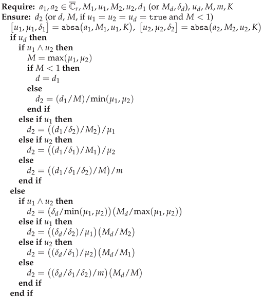 |
Besides the evaluations of and or of their factored representations, in the usual case, with , Algorithm d2byd1 needs three, four or four tests, and three, three or four divisions, for the cases when only or , or when , respectively; the case needs three tests, one ∧, one max and one min operations, and two divisions. If , an additional multiplication with is also required in all these four cases.
3.5. Direct Computation of
The direct computation of using its definition in (1),
needs to evaluate the reciprocals of and , then the difference , and finally the absolute value of this difference. The following algorithm shows how the reciprocal of a complex number a has to be safely computed. Note that if , , where can be given in a factored form, , but this product might not be representable. However, squaring up is prone to overflow, and therefore it must be avoided. Algorithm inva listed below shows how should be evaluated.
| Algorithm 5 inva computes the reciprocal of a complex number given its modulus or factored representation |
|
Remark 4.
The minus sign in front of ν is not necessary in this context, since the real and imaginary parts will be used to evaluate using Algorithm absa. Indeed, the signs of the imaginary parts of and do not matter.
Algorithm inva needs one test and four divisions if , or six divisions if , but it should be applied to both and . Therefore, two tests and eight, ten or twelve divisions are necessary if , and , for , , or , respectively. The remaining computations are the same as those for computing , but applied to . Therefore, the computational effort for computing using Algorithm inva shoud be compared to that of Algorithm d2byd1, which needs at most four tests and four divisions, or at most three tests, two divisions, one ∧, one max and one min operations, if ; if , another multiplication is needed.
Clearly, the direct approach needs more computations than the first approach, based on . Note that the first approach can easily and efficiently detect the case when is not needed, since its value will exceed . However, the direct approach has to be used when the first approach could not be used, namely, when overflows.
Remark 5.
The implementation inlines the low level algorithms, except for Algorithm
subtract, that is more involved; it is called two times, if can be found using , or four times, otherwise. Similarly, Algorithm inva
is either not called, or called twice. The very simple Algorithm absa
is called at most four times, and Algorithm d2byd1
is inlined once.
4. Numerical Results
This section starts by presenting four examples that show the significance of the proposed approach. Then, the numerical results obtained in a large experiment with randomly generated examples, which cover the entire range of representable numbers, are discussed. Finally, the performance of two solution approaches for a block diagonalization problem of order 999 is analyzed, illustrating the advantages of using a good eigenvalue reordering strategy and fast algorithms for computing the approximate symmetric chordal metric.
4.1. Detailed Examples
The numerical results for four examples are presented and compared with those got by the direct use of MATLAB computations.
Example 1.
Let , . Implementing formula (1) in MATLAB, the result is , while Algorithm
chordal, together to the lower level algorithms, returns 7.010041250456554e−309. Both and computed using (1) in MATLAB are wrong. Specifically, , with 1.617923821376084e+308, and the MATLAB command gives . Moreover, evaluating , it follows that , and therefore . On the other hand, the factored form of has and . Moreover, and , so that 1.004987562112089; therefore, .
Example 2.
Let 1.16e308 + 1.66e308 ı. MATLAB command
1/a
gives the result 0. While this is close to the true value, it is qualitatively wrong, since it does not satisfy the mathematical condition that . But using the factored form of , , with 1.66e308 and 1.219965042368649, as 1.16e308, it follows that
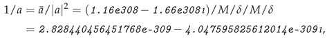 and then 9.999999999999996e−01 − 1.665334536937735e−16ı, which is very close to 1; the error is of the order of ε. Note that the denominator in (7) should be evaluated as shown there (or with permuted factors), but not as ; multiplying would give
Inf. Clearly, the result obtained is very close to 0, but it can be accurately obtained and it numerically verifies the condition on reciprocal of a complex number, while 0 does not. Note also that can be obtained directly as .
and then 9.999999999999996e−01 − 1.665334536937735e−16ı, which is very close to 1; the error is of the order of ε. Note that the denominator in (7) should be evaluated as shown there (or with permuted factors), but not as ; multiplying would give
Inf. Clearly, the result obtained is very close to 0, but it can be accurately obtained and it numerically verifies the condition on reciprocal of a complex number, while 0 does not. Note also that can be obtained directly as .
For computing in (1), it is necessary to evaluate both and , and then the absolute value of their difference. If and/or have real and imaginary parts with very big magnitude, as in Example 2, then using (1) will give an inaccurate result for d, as shown in the next example.
Example 3.
Let from Example 2, and . Implementing (1) in MATLAB, the result is 3.933412034978399e-309, while the implementation of Algorithm
chordal
gives 1.267129104195721e-309. The absolute difference between these values is very small, about
2.66628e-309. However, their relative difference, is about 0.67785, and taking as reference, . These big relative differences are due to the fact that using (1) to evaluate in MATLAB gives , and . Both MATLAB and Algorithm
chordal
compute 6.523894033771084e+307, but Algorithm
chordal
uses Algorihm
d2byd1
to obtain , where the factored representations are used for and .
Example 4.
Let . Using MATLAB, it follows that
1/a
= 0, which is wrong, since it implies that , while the true result is 1. On the contrary, Algorithm
inva
gives 5.134785827324312e-309 - 3.423190551549538e-309 ı. With this value, it follows that 1.000000000000000e+00 + 3.885780586188048e-16 ı, that has absolute and relative errors less than .
4.2. Large Experiment with Randomly Generated Examples
In a run with 4188166 random examples, the first three examples had , , and . Specifically, all examples have been generated using the following MATLAB commands, where a1 and a2 are used for and , respectively.
a1 = randn + 1i*randn; a2 = 0;
a2 = a1; a1 = 0;
a2 = 0;
for ii = -1022 : 1023
s1 = 2^ii; re = s1*randn; im = s1*randn;
if abs( re ) > realmax, re = sign( re )*realmax; end
if abs( im ) > realmax, im = sign( im )*realmax; end
a1 = re + 1i*im;
for jj = -1022 : 1023
s2 = 2^jj; re = s2*randn; im = s2*randn;
if abs( re ) > realmax, re = sign( re )*realmax; end
if abs( im ) > realmax, im = sign( im )*realmax; end
a2 = re + 1i*im;
end
end
s1 = realmax; re = s1*randn; im = s1*randn;
if abs( re ) > realmax, re = sign( re )*realmax; end
if abs( im ) > realmax, im = sign( im )*realmax; end
a1 = re + 1i*im;
for jj = -1022 : 1023
s2 = 2^jj; re = s2*randn; im = s2*randn;
if abs( re ) > realmax, re = sign( re )*realmax; end
if abs( im ) > realmax, im = sign( im )*realmax; end
a2 = re + 1i*im;
end
s2 = realmax; re = s2*randn; im = s2*randn;
if abs( re ) > realmax, re = sign( re )*realmax; end
if abs( im ) > realmax, im = sign( im )*realmax; end
a2 = re + 1i*im;
- The for loop with counter ii generates numbers s1 between (realmin) and 8.988465674311580e+307, which is very close to, but smaller than , (realmax), the relative error being smaller than 5.552e-17. The number s1 multiplies pseudorandom double precision values drawn from the standard normal distribution (with mean 0 and standard deviation 1), to obtain the real and imaginary parts of . If any of the computed parts of exceeds K in magnitude, i.e., if is obtained, that value is reset to . The number is obtained in the same way in the internal loop with counter jj. The second part of the code segment has and use it to obtain ; is generated as above. The last part also sets , and use it to obtain . Clearly, complex numbers with and/or are generated.
For reproductibility of the results, the command sequence above has been run after the MATLAB statement
rng( ’default’ )
- which ensures that the (initial) seed of the random number generator is the same, and therefore the same sequence of random numbers is generated after using this command. However, for some further tests, the generating sequence has been run repeateadly several times, but the rng( ’default’ ) command has been placed just before the first run. This way, a larger number of tests have been performed.
Inside the (internal) loops, an implementation of Algorithm chordal is called, and its results are compared with those obtained using a MATLAB command for (1), but also a more sophisticated MATLAB code based on algorithms described in Section 3. This is needed since using (1) directly might return inaccurate results, as shown in Section 4.1.
The maximum relative error in this run has been 6.3088e-16; the relative error is defined as , where d and denote the results obtained by evaluating (1) in MATLAB and by using an implementation of Algorithm chordal, respectively. If the absolute error is computed as , if , and , otherwise, its maximum has been 0.2649. The value became zero after a correction using a MATLAB code based on algorithms described in the previous section. After ten consecutive runs (without reinitialization of the random number generator), the maximum relative error and its mean value have been 7.6144e-16 and 6.3663e-16, respectively, while using the second definition, the values have been 0.73077 and 0.35080, and they became zero after correction.
In this test sequence, there were 3970109 examples with or negligible compared to the other, hence the logical variable f in Algorithm chordal was true. This represents 94.794% from the total number of examples. Specifically, 1985994 and 1984115 examples have and , respectively. From those with , 987937 have , 994601 have , and 3456 have . From examples with , 987834 have , 992853 have , and 3428 have . These categories correspond to the three cases, with , , and , respectively. For , the logical variables and , , have been true for all examples satisfying and , respectively. Moreover, for examples satisfying , when as well as needed to be computed, both and have been true. Using a factored representation has never been necessary for any of these 3970109 examples.
For the remaining 218055 examples, representing 5.206% of all examples, and are nonzero, distinct and relatively “close” to each other, since . Algorithm subtract has been used to compute the real and imaginary parts, and , of . For three and two examples, or , respectively, would exceed K in magnitude. For these five examples with , cannot be computed, hence , and consequently, needed to be directly computed calling twice Algorithm inva (for and ) and Algorithm subtract (for the real and imaginary parts of ). For the other 218050 examples, has been computed as , using Algorithm absa, and could be used to obtain via Algorithm d2byd1. Specifically, was true on input to absa, called for evaluating for 217980 examples, and it was false for the remaining 70 examples with expected overflow; but could be reset to true for 12 examples, for which could be evaluated as ; therefore, needed a factored representation, defined by and , for only 58 examples.
All these 218055 examples needed both and values. A factored representation for has been required for 56 examples. Although 21 examples were expected to require a factored representation for , the factors could be multiplied without overflows for nine of these examples.
Since could not be computed for five examples, due to expected overflows in or , it follows that can be found using Algorithm d2byd1 for 218050 examples. But for 107475 of them, with , was not computed, since , which implies that , hence . For 110517 examples, has been evaluated using , (or and ) and (or and ); therefore, for these examples, . Specifically, the case , when , happened for 110514 examples; the case and , when , and the case , when , appeared for just one and two examples, respectively. There was no case with and . For the remaining 58 examples for which needed a factored representation, defined by and , there were six cases with , 51 cases with and one case with . The corresponding formulas are , for , , and , respectively. The case with never appeared; for it, the formula would be , for .
Finally, for the five examples for which could not be computed, since or exceeded K, has been evaluated by calling Algorithm inva twice, for and . The logical variables and were true for four and one examples, respectively, and false for one and four examples. Therefore all formulas for and in Algorithm inva have been applied. Then, has been obtained using Algorithm subtract separately for the real and imaginary parts of ; the variable remained true for each of these examples. The result has been found by Algorithm absa.
These results show that all examples have been solved using the simplest possible formulas, which prove the efficiency of the implementation. Moreover, it was checked out that the results have been practically the same with those obtained when has been always computed using (6). This demonstrates that the accuracy of the results was preserved using the simplified formulas.
4.3. Block Diagonalization of a Matrix Pencil
This subsection summarizes the results obtained for block diagonalization of a matrix pencil of order , with 107 real and 446 complex conjugate eigenvalues, revealing dense clusters. The numerical approach has been briefly discussed in Section 1. Without using clustering information, a solution with 135 diagonal block pairs has been computed in 62.68 s (seconds). The largest block pair, of order 734, appeared in the 89-th block position on the diagonals; in addition, there are three and 131 diagonal block pairs. The remaining 104 real eigenvalues are included in the largest block pair.
Using an eigenvalue reordering strategy based on pairwise “distances” between eigenvalues, measured by the approximate symmetric chordal metric, another solution has been computed in 4.6905 s, hence the execution time has been 13.36 times shorter. More block pairs, specifically 141, have been found and the largest block pair, of order 719, appeared in the last position. This is the preferred situation, since well separated eigenvalues could be quickly placed in small block pairs in the leading part, while big clusters remain to be placed in the trailing part of the matrix pencil. There were 140 block pairs, and so, all real eigenvalues were available in the largest block pair. The efficiency gain is mainly due to a better eigenvalue reordering, which reduced the number of failed attempts to solve generalized Lyapunov equations. However, it is worth to mention that the number of “distances” between eigenvalues is , hence it increases quadratically with the problem size. Therefore, it is important that the algorithms for computing the approximate symmetric chordal metric be as fast as possible.
5. Conclusions
The basic theoretical properties of the approximate symmetric chordal metric for two real or complex numbers are investigated, and reliable, accurate and efficient algorithms for its computation are proposed. A factored representation of the modulus of a complex number is introduced, which allows to obtain very accurate results for the entire range of the floating point number system of a computer. Two different ways to evaluate the distance between the reciprocals of the given numbers are described. The algorithms can be easily implemented on various architectures and compilers. Extensive numerical tests have been performed to assess the performance of the associated implementation. The results have been compared to those obtained in MATLAB, but with appropriate modifications for numbers very close to the bounds of the range of representable values, where usual formulas give wrong results, as shown in several detailed numerical examples. A block diagonalization example is also discussed to illustrate the efficiency improvement possible using a proper eigenvalue reordering strategy and fast algorithms for computing the approximate symmetric chordal metric.
Funding
This research received no external funding.
Institutional Review Board Statement
Not applicable.
Informed Consent Statement
Not applicable.
Conflicts of Interest
The authors declare no conflicts of interest.
References
- Klamkin, M.S.; Meir, A. Ptolemy’s inequality, chordal metric, multiplicative metric. Pac. J. Math. 1982, 101, 389–392. [Google Scholar] [CrossRef]
- Sasane, A. A generalized chordal metric in control theory making strong stabilizability a robust property. Complex Anal. Oper. Theory 2013, 7, 1345–1356. [Google Scholar] [CrossRef]
- Papadimitrakis, M. Notes on Complex Analysis. 2019. Available online: http://fourier.math.uoc.gr/~papadim/complex_analysis_2019/gca_vvn_r.pdf (accessed on 3 May 2025).
- Rainio, O.; Vuorinen, M. Lipschitz constants and quadruple symmetrization by Möbius transformations. Complex Anal. Synerg. 2024, 20, 8. [Google Scholar] [CrossRef]
- Bishop, C. Complex Analysis I, MAT 536, Spring 2024. Stony Brook University, Dep Mathematics, 100 Nicolls Road, Stony Brook, NY 11794, 2024. [Google Scholar]
- Álvarez Tuñón, O.; Brodskiy, Y.; Kayacan, E. Loss it right: Euclidean and Riemannian metrics in learning-based visual odometry. arXiv 2023, arXiv:2401.05396v1 [cs.CV]. [Google Scholar] [CrossRef]
- Xu, W.; Pang, H.K.; Li, W.; Huang, X.; Guo, W. On the explicit expression of chordal metric between generalized singular values of Grassmann matrix pairs with applications. SIAM J. Matrix Anal. Appl. 2018, 39, 1547–1563. [Google Scholar] [CrossRef]
- Sun, J.-g. Perturbation theorems for generalized singular values. J. Comput. Math. 2025, 1, 233–242. [Google Scholar]
- Sasane, A. A refinement of the generalized chordal distance. SIAM J. Control & Optimiz. 2014, 52, 3538–3555. [Google Scholar] [CrossRef]
- Bavely, C.; Stewart, G.W. An algorithm for computing reducing subspaces by block diagonalization. SIAM J. Numer. Anal. 1979, 16, 359–367. [Google Scholar] [CrossRef]
- Golub, G.H.; Van Loan, C.F. Matrix Computations, fourth ed.; The Johns Hopkins University Press: Baltimore, Maryland, 2013. [Google Scholar]
- Wilkinson, J.H. The Algebraic Eigenvalue Problem; Oxford University Press (Clarendon): Oxford, UK, 1965. [Google Scholar]
- Wilkinson, J.H. Kronecker’s canonical form and the QZ algorithm. Lin. Alg. Appl. 1979, 28, 285–303. [Google Scholar] [CrossRef]
- Stewart, G.W. On the sensitivity of the eigenvalue problem Ax=λBx. SIAM J. Numer. Anal. 1972, 9, 669–686. [Google Scholar] [CrossRef]
- Demmel, J.W. The condition number of equivalence transformations that block diagonalize matrix pencils. SIAM J. Numer. Anal. 1983, 20, 599–610. [Google Scholar] [CrossRef]
- Kågström, B.; Westin, L. Generalized Schur methods with condition estimators for solving the generalized Sylvester equation. IEEE Trans. Automat. Contr. 1989, 34, 745–751. [Google Scholar] [CrossRef]
- Anderson, E.; Bai, Z.; Bischof, C.; Blackford, S.; Demmel, J.; Dongarra, J.; Du Croz, J.; Greenbaum, A.; Hammarling, S.; McKenney, A.; et al. LAPACK Users’ Guide: Third Edition; Software · Environments · Tools, SIAM: Philadelphia, 1999. [Google Scholar]
- MathWorks®. MATLAB™, Release R2024b.; The MathWorks, Inc.: 3 Apple Hill Drive, Natick, MA, 01760, 2024.
- Wolfram, S. The Story Continues: Announcing Version 14 of Wolfram Language and Mathematica, 2024. Available online: http://writings.stephenwolfram.com/2024/01/the-story-continues-announcing-version-14-of-wolfram-language-and-mathematica (accessed on 3 May 2025).
- Malcolm, M.A. Algorithms to reveal properties of floating-point arithmetic. Commun. ACM 1972, 15, 949–951. [Google Scholar] [CrossRef]
- Gentleman, W.M.; Marovich, S.B. More on algorithms that reveal properties of floating point arithmetic units. Commun. ACM 1974, 17, 276–277. [Google Scholar] [CrossRef]
- Boyd, S.; Vandenberghe, L. Convex Optimization; Cambridge University Press: Cambridge, United Kingdom, 2004. [Google Scholar]
Disclaimer/Publisher’s Note: The statements, opinions and data contained in all publications are solely those of the individual author(s) and contributor(s) and not of MDPI and/or the editor(s). MDPI and/or the editor(s) disclaim responsibility for any injury to people or property resulting from any ideas, methods, instructions or products referred to in the content. |
© 2025 by the authors. Licensee MDPI, Basel, Switzerland. This article is an open access article distributed under the terms and conditions of the Creative Commons Attribution (CC BY) license (http://creativecommons.org/licenses/by/4.0/).
Copyright: This open access article is published under a Creative Commons CC BY 4.0 license, which permit the free download, distribution, and reuse, provided that the author and preprint are cited in any reuse.


