
Submitted:
20 May 2025
Posted:
21 May 2025
You are already at the latest version
Abstract
Kolmogorov–Arnold Networks (KAN) represent a promising model suited for applications that require interpretability. Here, we explore the use of KAN to analyze time series of water quality parameters obtained from a published dataset related to an aquaponic environment. The Water Quality Index (WQI) was calculated as an arithmetic combination of three water parameters: pH, total dissolved solids, and temperature. By training KAN models, we derived explicit algebraic expressions capable of accurately predicting WQI, achieving low prediction error while emphasizing the most relevant predictors. Model performance was assessed using standard regression metrics, with R2 values exceeding 0.97 on the test set. These findings highlight the potential of KAN and its applicability to broader problems where accuracy, interpretability, and model simplification are desirable.
Keywords:
Kolmogorov-Arnold Networks
; Artificial Neural Networks
; Symbolic Regression
; Water Quality
; Aquaculture
1. Introduction
Kolmogorov-Arnold Networks (KAN) are a promising Artificial Neural Network (ANN) architecture recently proposed as a revolutionary paradigm [1,2]. KAN models possess valuable characteristics that can enhance accuracy and interpretability compared to traditional ANN models [3,4]. The interpretability characteristic of KAN is particularly noteworthy, which is achieved through the ability to derive closed mathematical expressions representing input-output relationships, commonly referred to as symbolic regression [5].
In this work, we apply KAN to analyze time series data collected from an Internet of Things (IoT)-based water quality monitoring system in an aquaponic environment [6]. The primary objective of this study is to evaluate the capability of KAN as a data-driven approach for automatically extracting symbolic expressions that effectively capture the relationship between input water parameters and the Water Quality Index (WQI). In this context, WQI is a composite target variable derived from the monitored parameters. Although multiple WQI formulations exist in the literature [7,8], our goal is not to analyze the index computations in depth. Instead, WQI is employed here as a representative use case to explore and illustrate key capabilities of KAN models, including the extraction of explicit mathematical input–output relationships and data-driven feature selection, all within a real-world application context.
The results demonstrate that the trained KAN model is able to predict WQI from the input parameters with satisfactory accuracy, as measured by Mean Absolute Error (MAE), Root Mean Squared Error (RMSE), and the coefficient of determination (R2) [9]. Additionally, we obtained a closed symbolic expression with predictive performance comparable to the trained model. Notably, the obtained symbolic expression slightly outperforms the original KAN model and reduces the number of input variables, highlighting its potential as a model simplification technique.
The findings from this case study emphasize KAN’s potential for applications that require interpretability and high model performance. In addition to automatically obtaining closed mathematical expressions representing input-output relationships, the results suggest that KAN can also serve as an effective feature extractor.
The remainder of this paper is structured as follows. Section 2 describes the dataset used as a case study, the preprocessing steps applied to the analyzed variables, and the computation of the WQI. It also introduces the fundamental concepts of KAN and details the specific model configuration and evaluation procedure employed in this study. Section 3 presents and discusses the main results, including model configuration, pruning, and the performance of symbolic expressions derived from the original and pruned KAN models. Finally, Section 4 presents the main conclusions, potential improvements, and directions for future work.
2. Material and Methods
2.1. Dataset Description
The dataset used in this study consists of water quality measurements collected from an aquaponic fish pond monitored with IoT sensors [6]. The monitored variables and their corresponding units are summarized in Table 1.
2.1.1. Data Cleaning and Preprocessing
IoT sensor networks, while enabling large-scale and continuous environmental monitoring, are prone to various data quality challenges [10]. Common issues include sensor malfunctions, power instability, intermittent connectivity, and communication failures. These problems often manifest as missing values, irregular sampling intervals, or noisy measurements. To address these challenges and ensure data reliability, appropriate cleaning and preprocessing steps are essential prior to any modeling or analysis [11,12].
In this study, the original dataset was not uniformly sampled, which required preprocessing to obtain a consistent time series structure. We selected a subset of the dataset covering the period from 2023-01-30 12:00:00 to 2023-02-08 16:00:00, representing more than nine consecutive days of monitoring. This subset comprises the complete dataset for analyses presented in this work.
We applied a mean aggregation procedure to resample the data at a 1-minute interval to achieve uniform temporal resolution. Despite this aggregation, some missing values remained due to irregularities in the original recordings. These gaps were addressed using second-order polynomial interpolation, which estimates the missing values by fitting a local quadratic curve to neighboring points.
Finally, to reduce sensor-induced noise and smooth short-term fluctuations, we applied a single-pole recursive Infinite Impulse Response (IIR) filter to each time series [13]. This step produced continuous, smoothed signals while preserving the broader trends relevant to subsequent modeling. The resulting preprocessed dataset is uniformly sampled, free of missing values, and smoothed, forming a consistent input for developing, training, and evaluating the models described in the following sections.
2.2. Weighted Arithmetic Water Quality Index
The Water Quality Index (WQI) is a widely used metric for assessing water quality [7,8]. Typically, such indices are calculated by mathematically combining measurements of water parameters. The calculation process generally involves the following steps: 1) variable selection, 2) parameter scaling, 3) weighting, and 4) algebraic aggregation [8]. Experts can assess water quality in specific contexts based on the computed index.
In this study, we used the Weighted Arithmetic Water Quality Index (WAWQI), referred to as WQI throughout the remainder of the manuscript for simplicity. Although various types of water quality indices are described in the literature [7,8], the weighted arithmetic WQI was chosen due to its simplicity and interpretability. The general formula of WQI is presented in Equation 1.
where:
- is the sub-index quality rating (scaled between 0 and 100).
- is the weight assigned to each variable.
Since the dataset includes three key variables (water pH, Total Dissolved Solids (TDS), and water temperature), each is mapped to a quality rating according to its specific characteristics, as described below.
2.2.1. Quality Rating Calculation
The quality rating for each variable is mapped to a value between 0 and 100 based on ideal and permissible values. The specific calculation for each parameter, as used in the present work, is described as follows:
pH quality rating (), equation 2
- = observed pH value
- Ideal pH = 7.0 (neutral)
- Standard maximum = 8.5
Inverse scaled TDS quality rating (), equation 3
- = observed TDS value
- Ideal TDS = 0 mg/L
- Standard maximum = 500 mg/L
- Higher TDS indicates worse quality (inverse scaling)
Temperature quality rating (), equation 4
- = observed water temperature
- Ideal temperature = 26°C
- Acceptable range = 24–27°C
- Deviation from 26°C results in a penalty
2.2.2. Weight Calculation
The weight for each variable is calculated as inversely proportional to its maximum permissible value, equation 5:
where:
- = standard limit for each variable
- k = proportionality constant (set to 1 for simplicity)
For this study, we used the following limits:
- (deviation range from 26°C)
By combining the quality ratings and weights according to Equation 1, the final WQI value is computed, providing a composite assessment of water quality based on the selected parameters. While the specific quality rating functions and thresholds adopted in this work suit the case study, alternative normalization schemes or WQI formulations could be employed to fit other applications. Such adjustments would not alter the core objectives of this study, which focus on evaluating the capabilities of KAN in modeling interpretable relationships from real-world water quality data.
2.3. Kolmogorov–Arnold Networks: Theoretical Foundations
Multilayer Perceptron (MLP) networks are based on the foundational principle that multilayer feedforward networks are universal approximators of any continuous function [14,15]. In contrast, Kolmogorov-Arnold Networks (KAN) are based on the Kolmogorov-Arnold superposition theorem (K-A theorem) [16,17].
The K-A theorem states that any multivariate continuous function , in wich , defined on a bounded domain, can be expressed as a combination of a finite number of continuous univariate functions. This formulation is mathematically described in equation 6.
where:
- - the target multivariate function to approximate.
- - the p-th input variable.
- - continuous univariate inner functions, applied to each input variable.
- - continuous univariate outer functions, combining the intermediate results.
- n - the dimensionality of the input space.
In practice, KAN implements this theoretical formulation by constructing a network where the inner functions () and outer functions () are approximated using neural network layers. This structure enables KAN to efficiently model complex relationships while retaining interpretability through the explicit mathematical expressions derived from the network’s learned functions.
2.4. KAN Implementation Details
The univariate functions and in Equation 6 are implemented in KAN as smooth, learnable functions constructed using a linear combination of basis functions known as B-splines [18]. B-splines are a specific class of spline functions that offer desirable properties such as local support, smoothness, and differentiability, making them particularly suitable for neural network training via backpropagation [19,20]. In practice, a univariate function within a KAN is represented as:
where is the i-th B-spline basis function of degree k, are learnable coefficients, and G is the number of grid intervals (also referred to as segments or knots) that define the piecewise structure.
In this study, we adopted a commonly used configuration of cubic B-splines () and selected intervals to balance model flexibility and computational efficiency, consistent with prior KAN implementations [1].
To represent the layered structure of a KAN, each layer is defined as a matrix whose entries are univariate functions mapping from input neuron i to output neuron j. Unlike traditional neural networks, where weights are scalar values, the connections in KAN are functional—each entry in the matrix is a spline-based function learned during training.
A KAN layer l is thus denoted as:
where and refer to the number of input and output units, respectively. Given an input vector , the operation of two consecutive KAN layers is expressed as:
where ∘ denotes function composition, not matrix multiplication. Each layer applies a learned set of univariate transformations to its inputs, sums them at the node level, and passes them to the next layer.
In this study, we implemented two models with the following configurations:
- Original model (KAN): Two layers configured as , , using all three input variables (pH, TDS, temperature).
- Pruned model (KAN′): Two layers configured as , , using only pH and temperature after feature sparsification.
As previously described, both models were trained to predict the WQI using their respective input configurations. The pruned model (KAN′) was obtained through a sparsification process that removed less relevant input features. Further details on this pruning strategy and its implications are provided in Section 3. Symbolic expressions were extracted from the learned univariate B-spline-based functions for each trained model. These expressions allow WQI predictions to be made without executing the whole network, showcasing a key strength of KAN: its ability to produce interpretable, compact mathematical representations of the modeled relationships. We computed MAE, RMSE, and metrics for both models and their corresponding symbolic expressions to evaluate performance.
2.4.1. Data Split
The available dataset was divided into training, validation, and testing subsets, following standard practices in machine learning workflows [21,22]. Since the preprocessed dataset was uniformly resampled at one-minute resolution, each day corresponds to samples.
- Training set: 6 complete days of data ( samples).
- Validation set: Approximately 1.5 days ( samples).
- Test set: Approximately 1.5 days ( samples).
This partitioning strategy supports a robust evaluation of model performance by separating the data used for training from the data used to monitor generalization and the final model assessment. The validation set was used during training to compute learning curves and guide model selection, while the test set was reserved exclusively for the final performance evaluation.
This approach helps mitigate a well-known problem in machine learning known as data leakage, which can lead to overly optimistic performance estimates if information from the test set inadvertently influences model training [23]. Maintaining a strict separation between these subsets ensures a reliable evaluation pipeline aligned with best practices in data-driven modeling.
2.5. Overview of the Proposed Methodology
Figure 1 presents a flowchart that summarizes the methodology adopted in this study. The workflow begins with acquiring raw data from a publicly available IoT-based dataset [6], which includes water quality measurements such as pH, TDS, and temperature.
The data were subjected to a series of pre-processing steps to ensure consistency and reliability. First, a 1-minute mean aggregation was applied to achieve uniform temporal resolution. Subsequently, missing values were imputed using second-order polynomial interpolation. A single-pole IIR smoothing filter was applied to reduce noise typically introduced by low-cost IoT sensors.
Following preprocessing, two Kolmogorov–Arnold Network (KAN) models were trained: the complete model using all three input variables (pH, TDS, and temperature), and a pruned model using only the most relevant features identified via sparsification. Symbolic regression was then performed to extract interpretable expressions from each trained model.
Finally, both model-based predictions and symbolic expressions were evaluated using standard regression metrics, including MAE, RMSE, and , to assess predictive performance and compare original and pruned models.
3. Results and Discussion
The time series of water quality parameters and the computed WQI over the study period (January 30 to February 8, 2023) are presented in Figure 2. The top panel shows the WQI values, with visual markers indicating the training (blue), validation (orange), and test (purple) intervals. Subsequent panels display the time series for pH, TDS, and temperature, respectively. Color-coded lines facilitate clear visual differentiation of each parameter. These signals were processed using the steps described in Section 2.1.1, including temporal aggregation, imputation of missing values, and smoothing, to ensure the reliability of input data for model development. These preprocessing procedures were crucial to mitigate common data quality issues associated with IoT sensor systems—such as noise, missing values, and temporal irregularities—which are well documented in the literature [10,11,12,24].
3.1. Architectures of the Original and Pruned KAN Models
Figure 3 depicts the architecture of the original and pruned KAN models used to predict WQI. The original model (KAN) includes three input variables—pH, TDS, and temperature—while the pruned model (KAN′) uses only pH and temperature. The reduction was guided by a sparsification process that eliminates non-contributing neurons and B-spline functions during training. This method results in a compact subnetwork, indicated by the darker nodes and edges in the diagram, representing the active components relevant to prediction.
The sparsification technique leverages the flexibility of learnable univariate B-spline-based functions, allowing KAN to discard less informative inputs automatically. This enhances model interpretability while improving computational efficiency. In this case, the TDS variable was identified as non-essential and removed in the pruned configuration. Despite this simplification, KAN′ demonstrated superior predictive performance, as detailed in Section 3.2. These findings underscore the value of KAN’s built-in variable selection capability, particularly for applications requiring streamlined sensor setups or reduced input dimensionality.
The symbolic functions extracted from each model reveal how KAN captures interpretable relationships between input parameters and the WQI. In both cases, the resulting expressions were linear, aligning with the WQI’s underlying formulation described in Equation 1. This confirms that the model successfully identified the expected input–output structure, echoing results observed in other domains [4,5].
Interestingly, the pruned model not only retained its predictive accuracy, as shown in Section 3.2, but also provided a key insight: the WQI—originally calculated using three input variables—could be reliably predicted using only pH and temperature. This finding has practical implications for deployment in IoT-based monitoring systems, as it reduces the number of required sensors, thereby lowering equipment and maintenance costs. While traditional WQI estimation typically depends on expert-defined parameters, data-driven methods such as KAN offer a scalable and interpretable alternative, particularly when sensor data are continuously available. We conducted an exploratory analysis of variable relationships using correlation and mutual information metrics to understand further the statistical dependencies that may have influenced KAN’s feature selection behavior.
3.1.1. Exploratory Analysis of Variable Relationships
To complement the insights gained from the model pruning process, we conducted an exploratory analysis of pairwise relationships between the input variables (pH, TDS, and temperature) and the WQI. Figure 4 presents two heatmaps: the left panel displays Pearson correlation coefficients, which capture linear associations, while the right panel shows normalized mutual information (MI), capable of revealing both linear and nonlinear dependencies. The combined use of correlation and mutual information is a well-established strategy in machine learning for feature relevance assessment, offering complementary perspectives on variable interactions [25]. This analysis used only the training and validation sets to prevent data leakage and ensure the integrity of subsequent model evaluation.
The results show a strong linear correlation between pH and WQI (), and moderate correlations between temperature and both WQI () and TDS (). In contrast, TDS exhibits almost no correlation with WQI (). The normalized MI matrix provides additional perspective, revealing moderate shared information between WQI and both pH (0.36) and temperature (0.36), while TDS again shows limited relevance (0.18).
These results support the sparsification-driven selection by the KAN model: pH and temperature appear to carry more informative content for predicting WQI, while TDS contributes little. Notably, despite being used in the original WQI computation, TDS was effectively discarded by the pruned KAN model—highlighting the model’s ability to perform implicit feature selection in a data-driven manner.
Interestingly, the mutual information between temperature and WQI also aligns with qualitative observations from the time series in Figure 2, where daily temperature oscillations seem to propagate into the WQI trend subtly. This is expected, as WQI is computed from normalized ratings that may amplify such cyclical patterns even if their original contribution is moderate.
Together, these findings demonstrate that the reduced model provides both interpretability and computational efficiency, while also exhibiting strong alignment with the dataset’s underlying statistical structure and visual patterns.
3.2. Model Inference and Symbolic Expression Evaluation
3.2.1. Symbolic Formulas
The symbolic expressions obtained from the trained KAN models are presented in equations 9 and 10. These expressions mathematically represent the relationship between the input variables (pH, temperature, and TDS) and the output (WQI).
In the equations above, , , , and y represent pH, temperature, TDS, and WQI, respectively. The symbolic expressions derived from both models demonstrate a close numerical similarity. Notably, the weight attributed to TDS () in Equation 9 is 0.002, indicating a negligible contribution from this variable. This minimal impact on WQI prediction justifies its exclusion in the pruned model. Consequently, the pruned expression in Equation 10 remains quantitatively consistent with the original, further validating the model simplification.
3.2.2. Performance Evaluation
The performance of the trained KAN models and the predictive capacity of the obtained symbolic expressions can be visually represented in Figure 5. As shown, both KAN models (original and pruned) and their respective symbolic expressions closely resemble the observed dynamics of WQI in the test set. However, the pruned model visually demonstrates better performance, as indicated by the closer alignment between the predicted and true WQI values.
Table 2 presents a quantitative assessment of both models and their symbolic equivalents using the coefficient of determination (), MAE, and RMSE.
The results presented in Table 2 indicate that:
- The pruned model, trained with reduced input variables, demonstrates enhanced accuracy compared to the original model.
- The pruned model shows slightly better generalization on the test set, as evidenced by a higher and lower MAE and RMSE values. This highlights the capability of KAN models to effectively eliminate less relevant variables while maintaining or improving predictive performance.
- The symbolic expressions obtained from both models (original and pruned) offer improved interpretability and enable the optimization of sensor deployment by reducing the number of measurements required. This practical advantage translates into lower equipment, installation, and maintenance costs, while achieving better predictive accuracy in the case study analyzed in this work.
These findings underscore the potential of KAN models as interpretable and accurate data-driven solutions for water quality monitoring and other applications where feature selection and interpretability are essential. Given that this study utilized a dataset related to aquaponics, a subfield of aquaculture, and considering the significant role of WQI in the aquaculture industry [26], the presented results demonstrate practical relevance. Moreover, our approach aligns with previous studies in aquaculture that emphasize interpretability and the use of easily implementable techniques [27,28].
4. Conclusions
In this work, we applied Kolmogorov-Arnold Networks (KAN) to predict the Weighted Arithmetic Water Quality Index (WQI) calculated as a linear combination of normalized water quality parameters (pH, TDS, and temperature). The dataset used in this case study was collected from an aquaponic environment using IoT sensors. We presented two KAN models: the original model, which utilized all three input variables, and a pruned version, which employed only pH and temperature as inputs after feature selection guided by sparsification.
Both models effectively captured the linear input-output relationship between the water quality parameters and the WQI. Notably, the pruned model demonstrated slightly better predictive performance while maintaining high accuracy, despite the reduction in input variables. The symbolic expressions derived from each model also demonstrated robust prediction capabilities, achieving regression metrics such as above 0.98. This result highlights the potential of the pruned model not only for maintaining predictive accuracy but also for optimizing sensor deployment, which is advantageous for practical applications by reducing operational costs. The results support using KAN as a valuable approach for scenarios where interpretability and simplicity are essential. The pruned model demonstrated practical advantages in the specific case of water quality monitoring in aquaculture environments, offering a simplified yet accurate modeling strategy.
Future work may explore the application of KAN in more complex scenarios, such as non-linear problem settings, classification tasks, and comparisons with other established neural network architectures like Multilayer Perceptrons (MLPs). Additionally, extending this approach to forecast future values in time series analysis could further demonstrate the versatility of KAN models.
Funding
This research received no external funding.
Institutional Review Board Statement
Not applicable.
Data Availability Statement
The original data presented in the study are openly available in: https://data.mendeley.com/datasets/yd36bx6f8f.
Conflicts of Interest
The authors declare no conflicts of interest.
References
- Liu, Z.; Wang, Y.; Vaidya, S.; Ruehle, F.; Halverson, J.; Soljačić, M.; Hou, T.Y.; Tegmark, M. KAN: Kolmogorov-Arnold Networks, 2024. [CrossRef]
- Liu, Z.; Ma, P.; Wang, Y.; Matusik, W.; Tegmark, M. KAN 2.0: Kolmogorov-Arnold Networks Meet Science, 2024. [CrossRef]
- Ji, T.; Hou, Y.; Zhang, D. A Comprehensive Survey on Kolmogorov Arnold Networks (KAN), 2024. [CrossRef]
- Gilbert Zequera, R.A.; Rassõlkin, A.; Vaimann, T.; Kallaste, A. Kolmogorov-Arnold networks for algorithm design in battery energy storage system applications. Energy Reports 2025, 13, 2664–2677. [Google Scholar] [CrossRef]
- Huang, Y.; Li, B.; Wu, Z.; Liu, W. Symbolic Regression Based on Kolmogorov–Arnold Networks for Gray-Box Simulation Program with Integrated Circuit Emphasis Model of Generic Transistors. Electronics 2025, 14, 1161. [Google Scholar] [CrossRef]
- Siswanto, B.; Dani, Y.; Morika, D.; Mardiyana, B. A simple dataset of water quality on aquaponic fish ponds based on an internet of things measurement device. Data in Brief 2023, 48, 109248. [Google Scholar] [CrossRef]
- Uddin, M.G.; Nash, S.; Olbert, A.I. A review of water quality index models and their use for assessing surface water quality. Ecological Indicators 2021, 122, 107218. [Google Scholar] [CrossRef]
- Chidiac, S.; El Najjar, P.; Ouaini, N.; El Rayess, Y.; El Azzi, D. A comprehensive review of water quality indices (WQIs): history, models, attempts and perspectives. Reviews in Environmental Science and Bio/Technology 2023, 22, 349–395. [Google Scholar] [CrossRef]
- Chicco, D.; Warrens, M.J.; Jurman, G. The coefficient of determination R-squared is more informative than SMAPE, MAE, MAPE, MSE and RMSE in regression analysis evaluation. PeerJ Computer Science 2021, 7, e623. [Google Scholar] [CrossRef]
- Krishnamurthi, R.; Ku"March", A.; Gopinathan, D.; Nayyar, A.; Qureshi, B. An Overview of IoT Sensor Data Processing, Fusion, and Analysis Techniques. Sensors 2020, 20, 6076. [Google Scholar] [CrossRef]
- Liu, Y.; Dillon, T.; Yu, W.; Rahayu, W.; Mostafa, F. Missing Value Imputation for Industrial IoT Sensor Data With Large Gaps. IEEE Internet of Things Journal 2020, 7, 6855–6867. [Google Scholar] [CrossRef]
- França, C.M.; Couto, R.S.; Velloso, P.B. Missing Data Imputation in Internet of Things Gateways. Information 2021, 12, 425. [Google Scholar] [CrossRef]
- Cao, L. Practical Issues in Implementing a Single-Pole Low-Pass IIR Filter [Applications Corner]. IEEE Signal Processing Magazine 2010, 27, 114–117. [Google Scholar] [CrossRef]
- Hornik, K.; Stinchcombe, M.; White, H. Multilayer feedforward networks are universal approximators. Neural Networks 1989, 2, 359–366. [Google Scholar] [CrossRef]
- Leshno, M.; Lin, V.Y.; Pinkus, A.; Schocken, S. Multilayer feedforward networks with a nonpolynomial activation function can approximate any function. Neural Networks 1993, 6, 861–867. [Google Scholar] [CrossRef]
- Schmidt-Hieber, J. The Kolmogorov–Arnold representation theorem revisited. Neural Networks 2021, 137, 119–126. [Google Scholar] [CrossRef]
- Vaca-Rubio, C.J.; Blanco, L.; Pereira, R.; Caus, M. Kolmogorov-Arnold Networks (KANs) for Time Series Analysis, 2024. [CrossRef]
- Abueidda, D.W.; Pantidis, P.; Mobasher, M.E. DeepOKAN: Deep operator network based on Kolmogorov Arnold networks for mechanics problems. Computer Methods in Applied Mechanics and Engineering 2025, 436, 117699. [Google Scholar] [CrossRef]
- Perperoglou, A.; Sauerbrei, W.; Abrahamowicz, M.; Schmid, M. A review of spline function procedures in R. BMC Med. Res. Methodol. 2019, 19, 46. [Google Scholar] [CrossRef]
- Hasan, M.S.; Alam, M.N.; Fayz-Al-Asad, M.; Muhammad, N.; Tunç, C. B-spline curve theory: An overview and applications in real life. Nonlinear Engineering 2024, 13, 20240054. [Google Scholar] [CrossRef]
- Xu, Y.; Goodacre, R. On Splitting Training and Validation Set: A Comparative Study of Cross-Validation, Bootstrap and Systematic Sampling for Estimating the Generalization Performance of Supervised Learning. Journal of Analysis and Testing 2018, 2, 249–262. [Google Scholar] [CrossRef]
- Joseph, V.R. Optimal ratio for data splitting. Statistical Analysis and Data Mining: The ASA Data Science Journal 2022, 15, 531–538. [Google Scholar] [CrossRef]
- Kapoor, S.; Narayanan, A. Leakage and the reproducibility crisis in machine-learning-based science. Patterns 2023, 4, 100804. [Google Scholar] [CrossRef]
- Abbasian Dehkordi, S.; Farajzadeh, K.; Rezazadeh, J.; Farahbakhsh, R.; Sandrasegaran, K.; Abbasian Dehkordi, M. A survey on data aggregation techniques in IoT sensor networks. Wireless Networks 2019, 26, 1243–1263. [Google Scholar] [CrossRef]
- Zhou, H.; Wang, X.; Zhu, R. Feature selection based on mutual information with correlation coefficient. Applied Intelligence 2022, 52, 5457–5474. [Google Scholar] [CrossRef]
- Do, D.D.; Le, A.H.; Vu, V.V.; Le, D.A.N.; Bui, H.M. Evaluation of water quality and key factors influencing water quality in intensive shrimp farming systems using principal component analysis-fuzzy approach. Desalination and Water Treatment 2025, 321, 101002. [Google Scholar] [CrossRef]
- Ferreira, N.; Bonetti, C.; Seiffert, W. Hydrological and Water Quality Indices as management tools in marine shrimp culture. Aquaculture 2011, 318, 425–433. [Google Scholar] [CrossRef]
- Tallar, R.Y.; Suen, J.P. Aquaculture Water Quality Index: a low-cost index to accelerate aquaculture development in Indonesia. Aquaculture International 2015, 24, 295–312. [Google Scholar] [CrossRef]
Figure 1.
Flowchart of the proposed methodology. The pipeline starts with raw data collected from IoT sensors and proceeds through preprocessing, KAN training, symbolic regression, and model evaluation.
Figure 1.
Flowchart of the proposed methodology. The pipeline starts with raw data collected from IoT sensors and proceeds through preprocessing, KAN training, symbolic regression, and model evaluation.

Figure 2.
Time series of water quality variables (pH, TDS, and temperature) and the WQI over the study period. The WQI plot highlights training, validation, and test data splits.
Figure 2.
Time series of water quality variables (pH, TDS, and temperature) and the WQI over the study period. The WQI plot highlights training, validation, and test data splits.
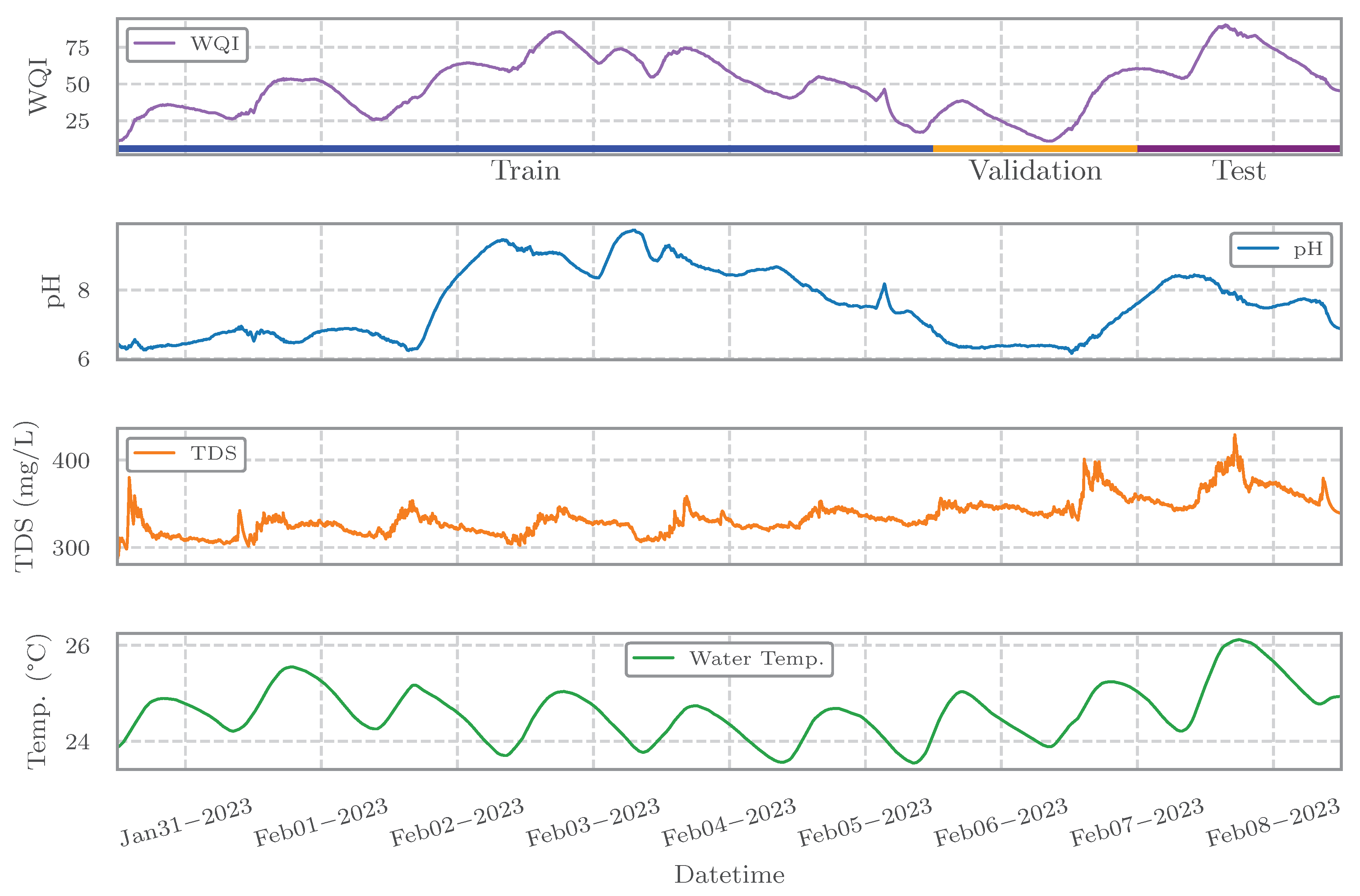
Figure 3.
Structure of the original (left) and pruned (right) KAN models used for WQI prediction. Darker nodes and edges indicate active components retained after sparsification.
Figure 3.
Structure of the original (left) and pruned (right) KAN models used for WQI prediction. Darker nodes and edges indicate active components retained after sparsification.
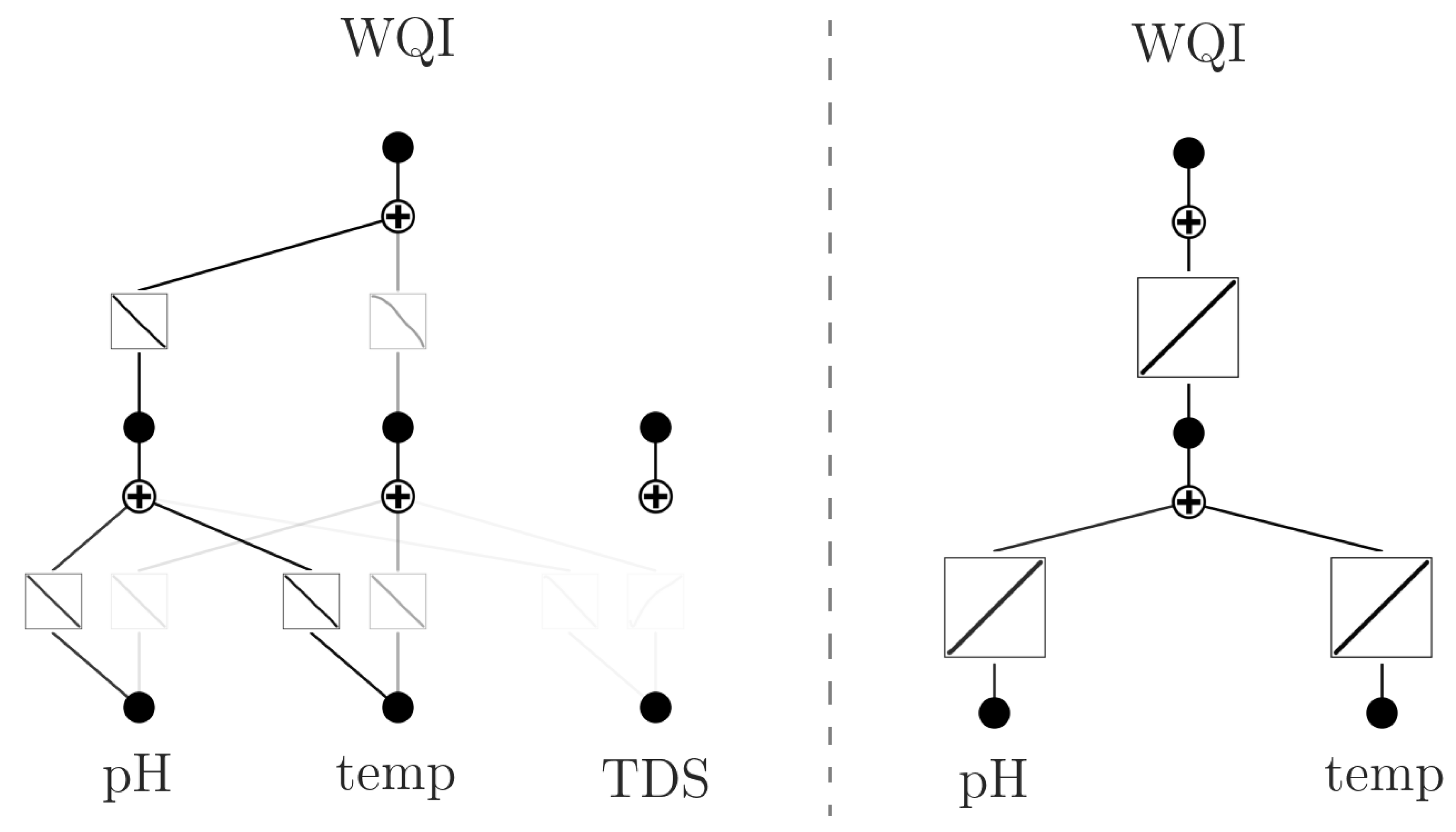
Figure 4.
Left: Correlation coefficients among water quality parameters and WQI. Right: Normalized mutual information (MI), symmetrized and scaled to [0, 1]. Both analyses were based on training and validation data.
Figure 4.
Left: Correlation coefficients among water quality parameters and WQI. Right: Normalized mutual information (MI), symmetrized and scaled to [0, 1]. Both analyses were based on training and validation data.
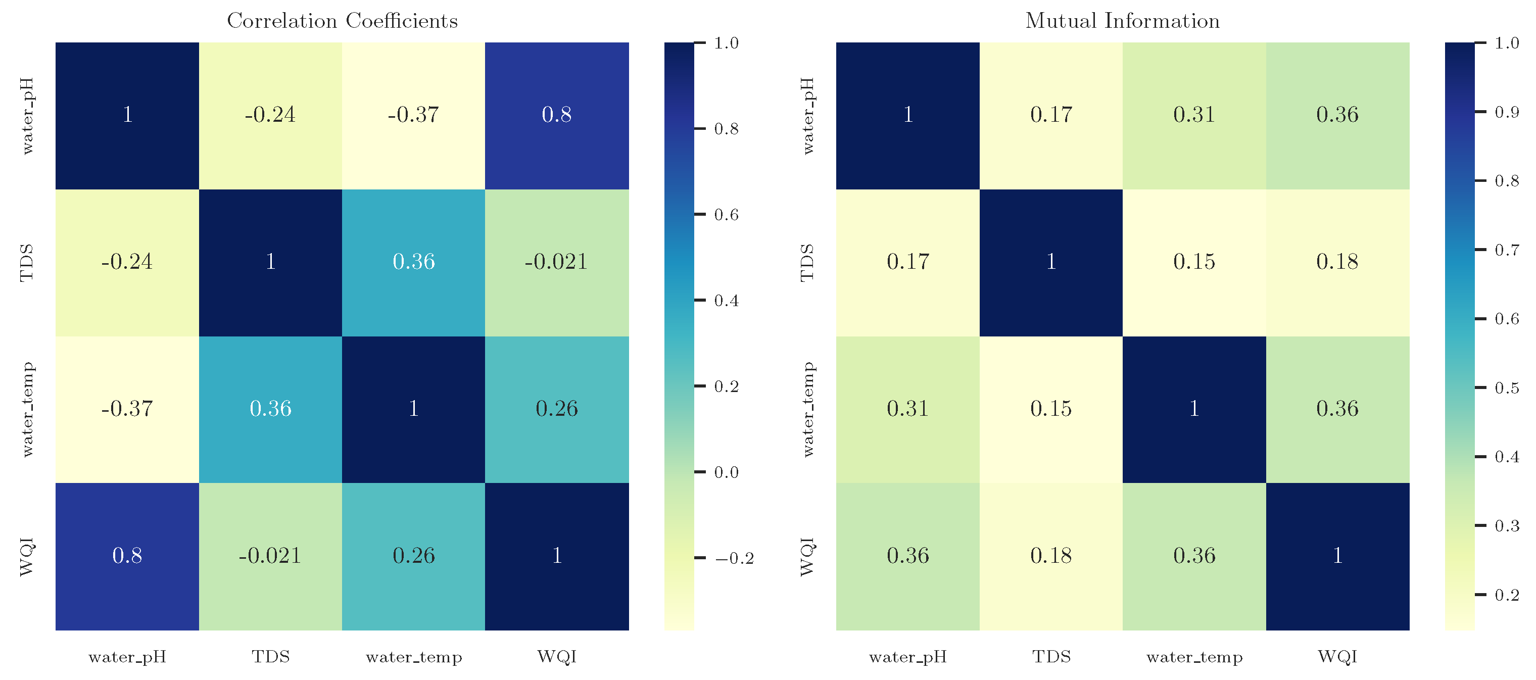
Figure 5.
Comparison of model predictions and symbolic expressions with the observed WQI over the test period. The pruned model and its symbolic expression demonstrate improved accuracy compared to the original model.
Figure 5.
Comparison of model predictions and symbolic expressions with the observed WQI over the test period. The pruned model and its symbolic expression demonstrate improved accuracy compared to the original model.
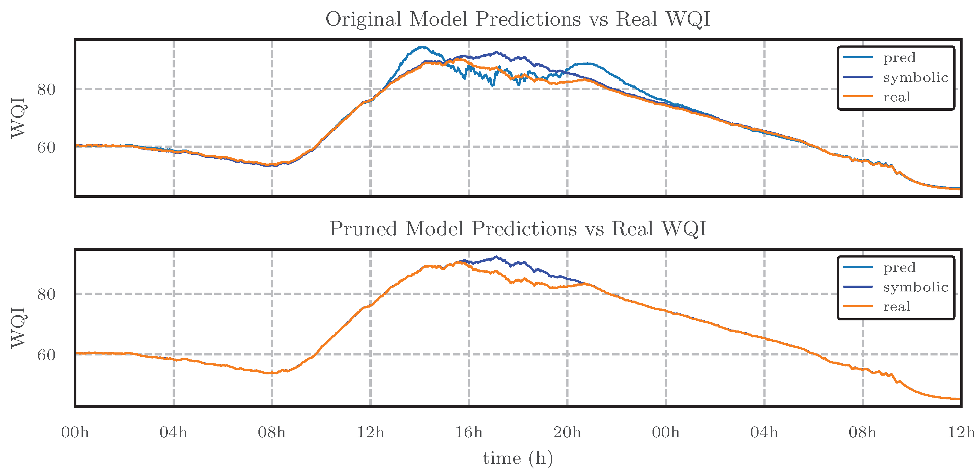

Table 1.
Water quality variables and their units as measured by IoT sensors.
| Description | Units |
|---|---|
| Timestamp recorded | DateTime |
| Water pH | pH units |
| TDS concentration | mg/L (ppm) |
| Water temperature | °C (Celsius) |
Table 2.
Performance metrics for model inference and symbolic predictions on the test set.
| Model | R² Score | MAE | RMSE |
|---|---|---|---|
| Original Model (inference) | 0.970 | 1.236 | 2.203 |
| Symbolic Prediction - Original Model | 0.982 | 0.806 | 1.722 |
| Pruned Model (inference) | 0.987 | 0.520 | 1.471 |
| Symbolic Prediction - Pruned Model | 0.987 | 0.520 | 1.471 |
Disclaimer/Publisher’s Note: The statements, opinions and data contained in all publications are solely those of the individual author(s) and contributor(s) and not of MDPI and/or the editor(s). MDPI and/or the editor(s) disclaim responsibility for any injury to people or property resulting from any ideas, methods, instructions or products referred to in the content. |
© 2025 by the authors. Licensee MDPI, Basel, Switzerland. This article is an open access article distributed under the terms and conditions of the Creative Commons Attribution (CC BY) license (http://creativecommons.org/licenses/by/4.0/).
Copyright: This open access article is published under a Creative Commons CC BY 4.0 license, which permit the free download, distribution, and reuse, provided that the author and preprint are cited in any reuse.


